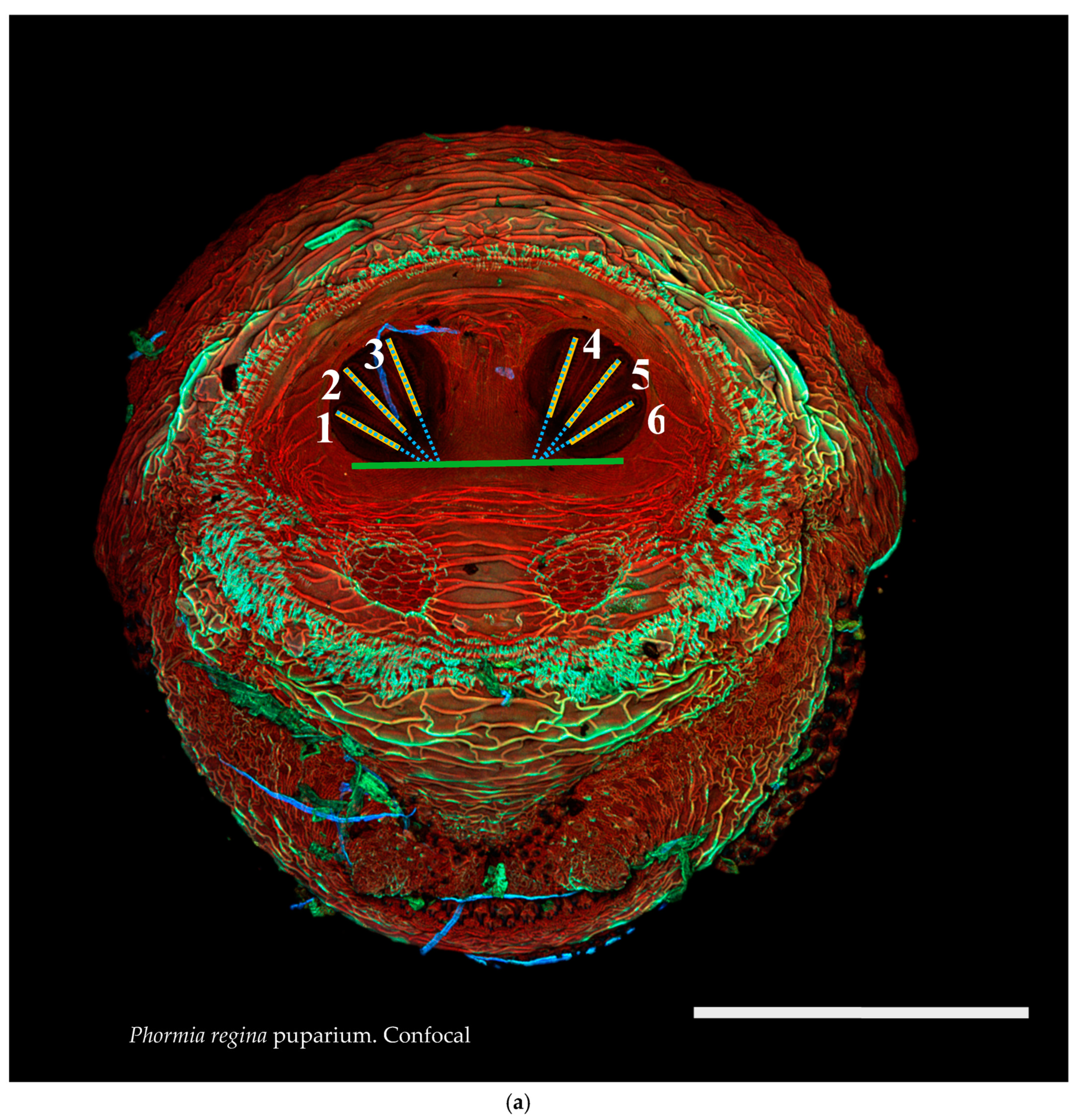
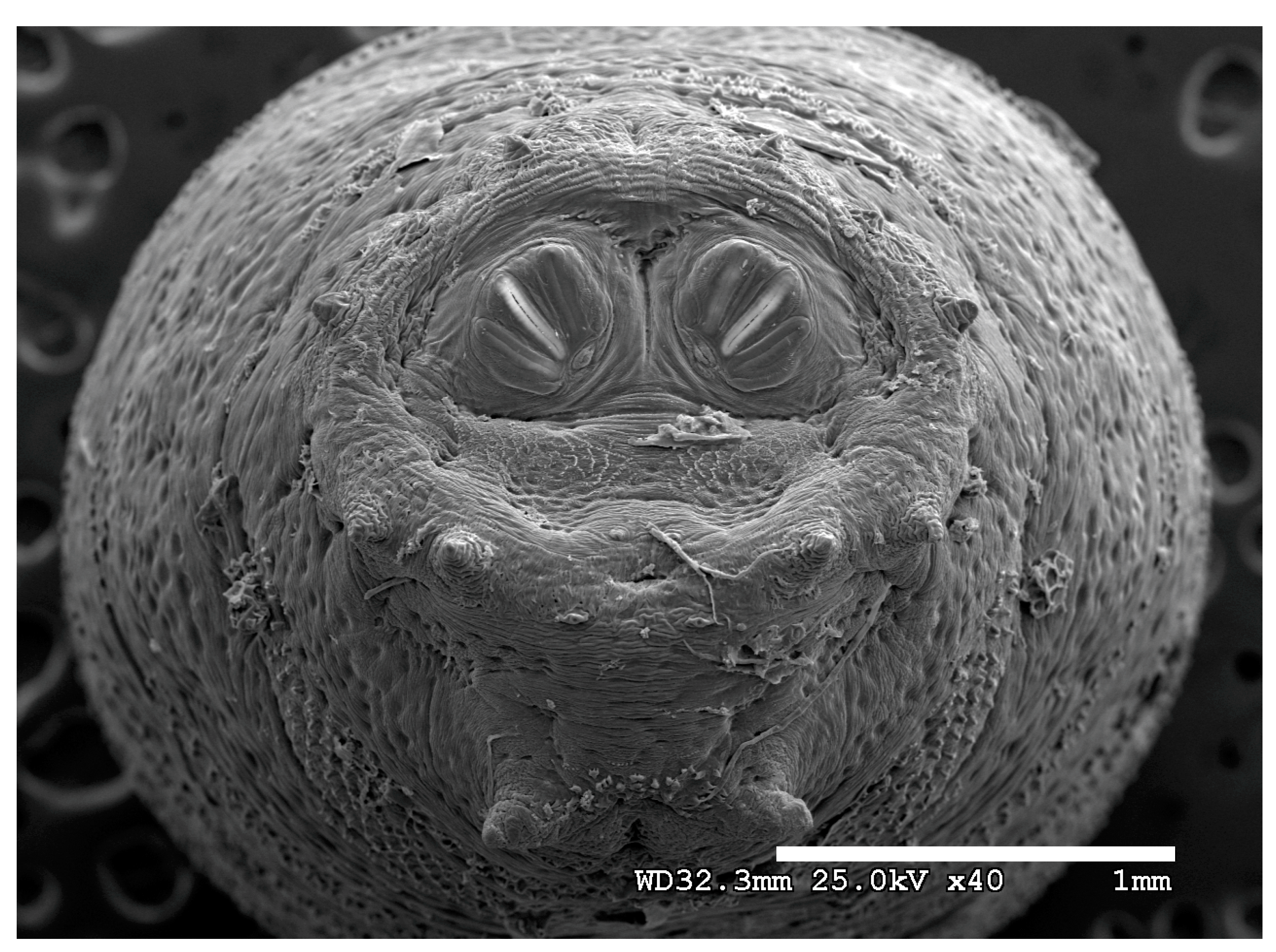
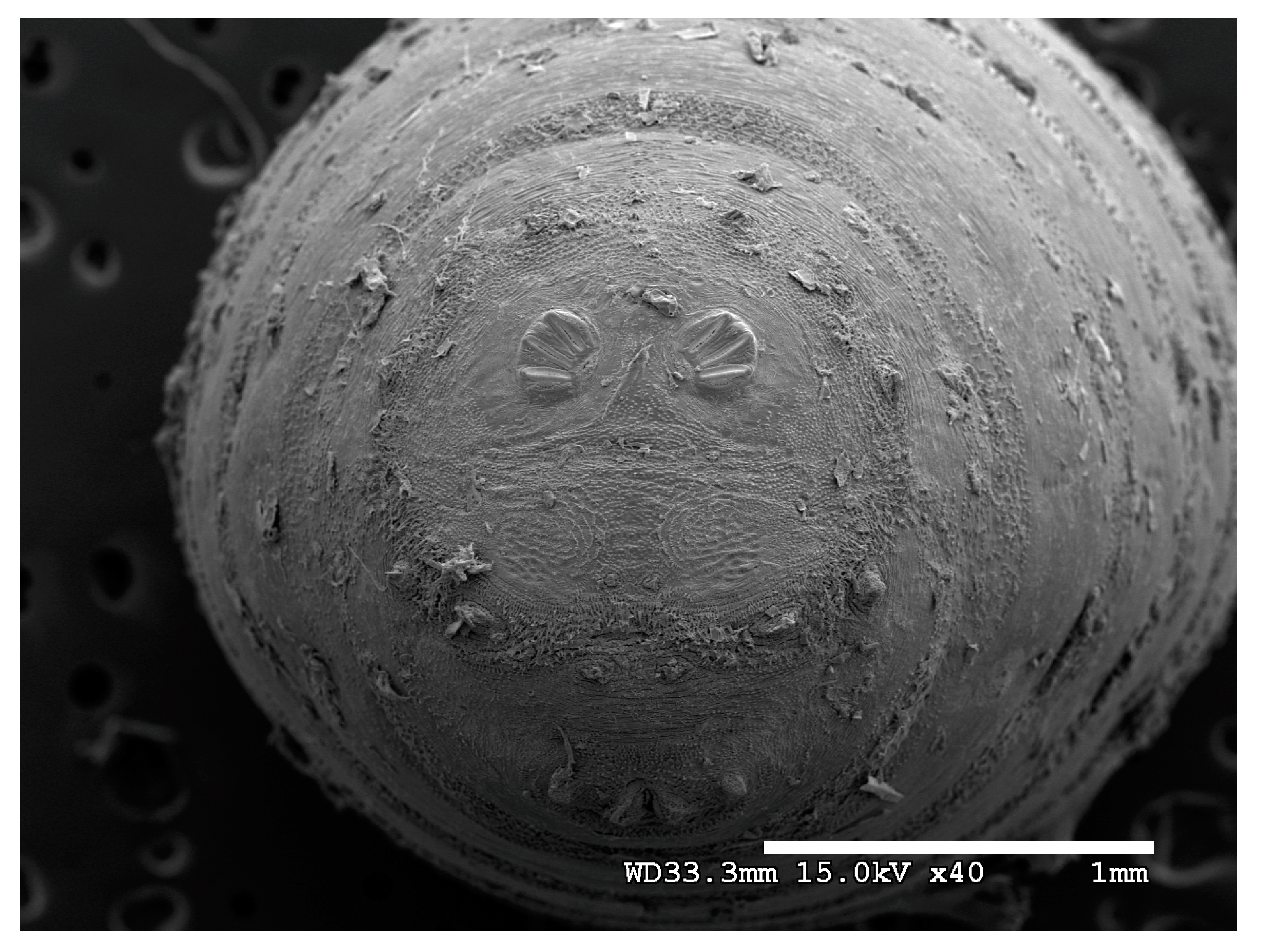
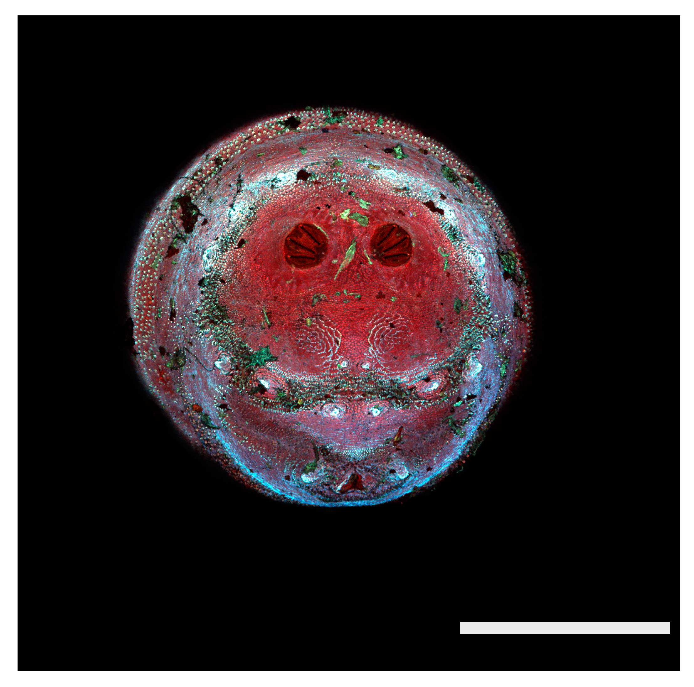
Figure 1.
Phormia regina puparium. Confocal maximum intensity projection at 40×, scale bar is 1 mm. Coordinates for start and stop points (points 1–12) on spiracular slits are reported and used for morphometric calculations.
Figure 1.
Phormia regina puparium. Confocal maximum intensity projection at 40×, scale bar is 1 mm. Coordinates for start and stop points (points 1–12) on spiracular slits are reported and used for morphometric calculations.
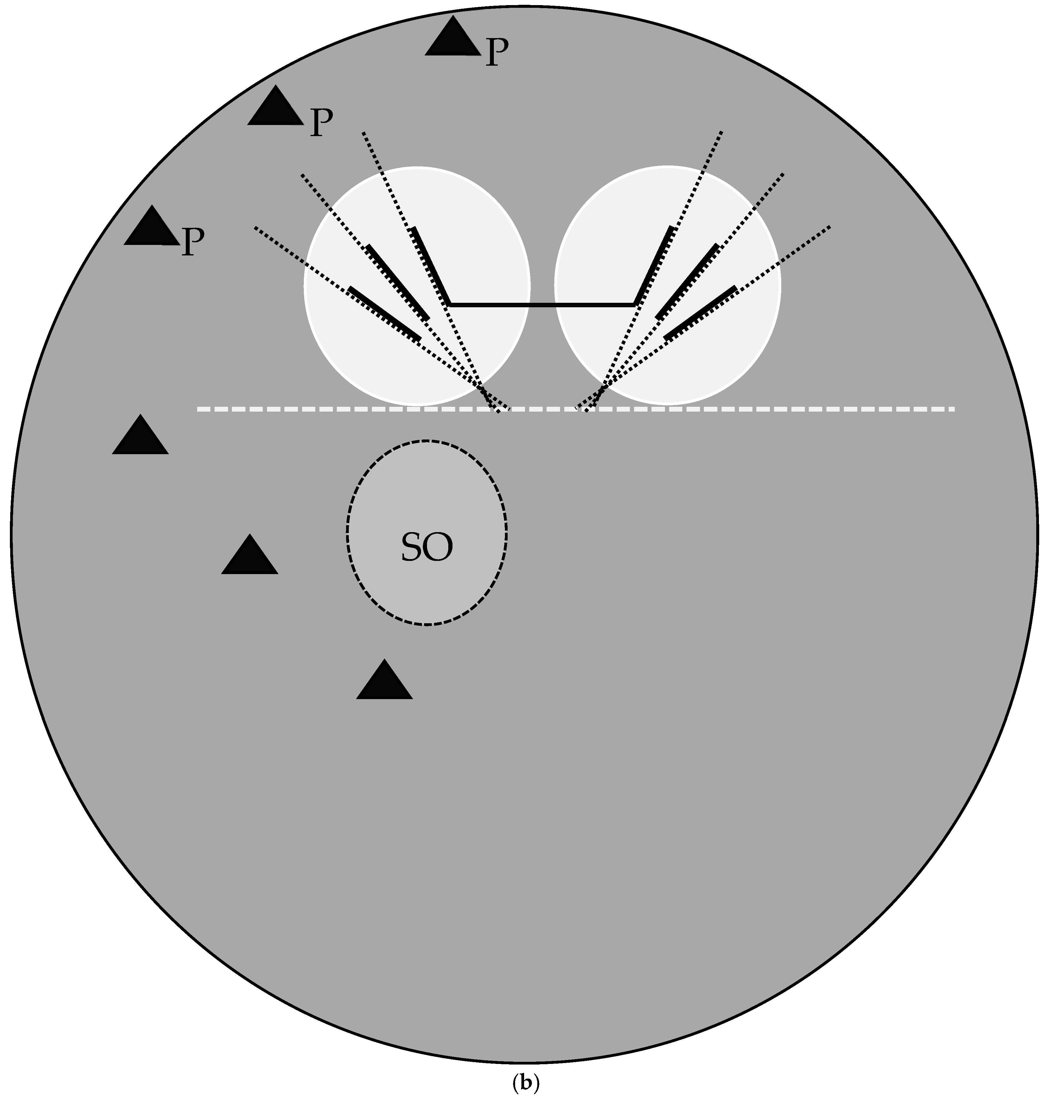
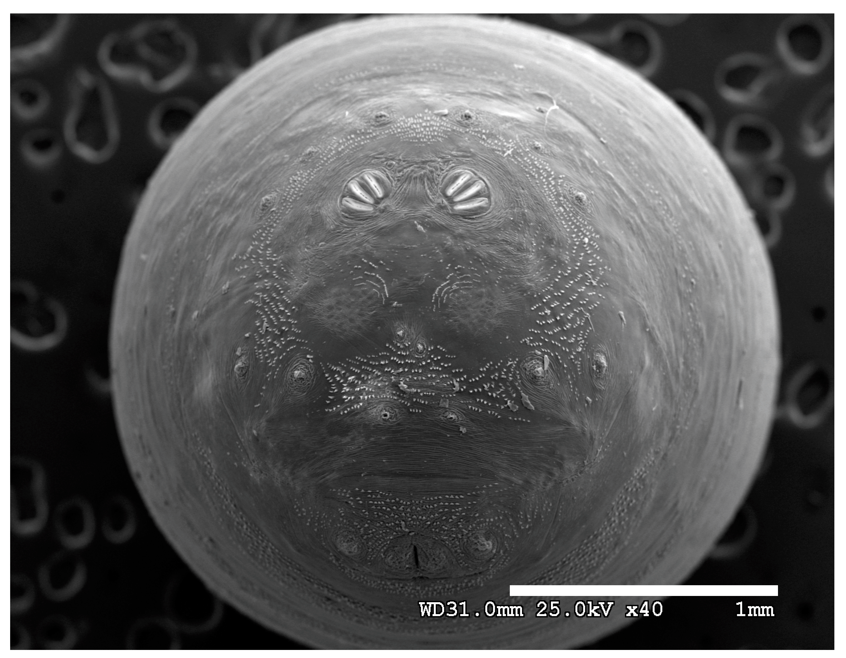
Figure 2.
(a) Cochliomyia macellaria puparium. Confocal maximum intensity projection at 40×, scale bar is 1 mm. Green line is a representation of the 180-degree line set by the ImageJ 1.0 macro from user input. Quantification of angles (blue dashed lines) and length of spiracular slits from position 1 to 6. (b) Diagram of measurements and calculations. Dotted gray line is user-set horizontal or 180°; dotted black lines indicate calculated angles. Thick black lines are length measurements of spiracular slit start and stop points. Horizontal black line is calculated distances based on start and stop points reported by ImageJ. Black triangles are papillae. SO: spiracular operculum (scored as easily viewed [1>] or not [0]). P: papillae (scored as not easily visible [0], visible [1], or large [2]).
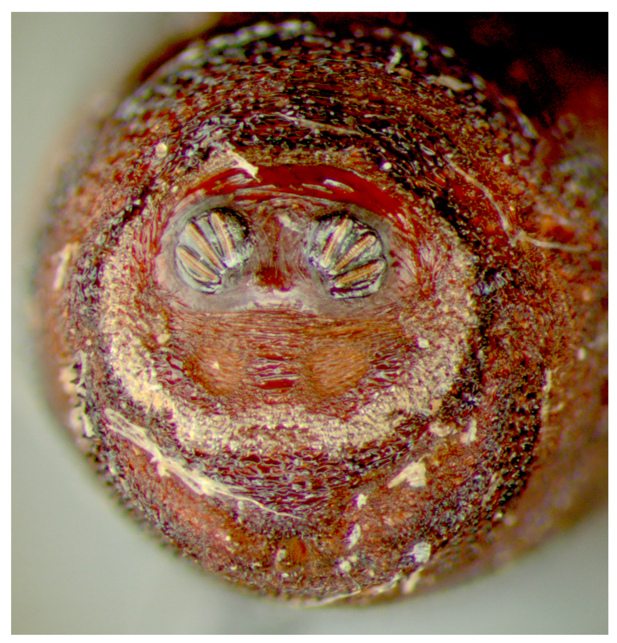
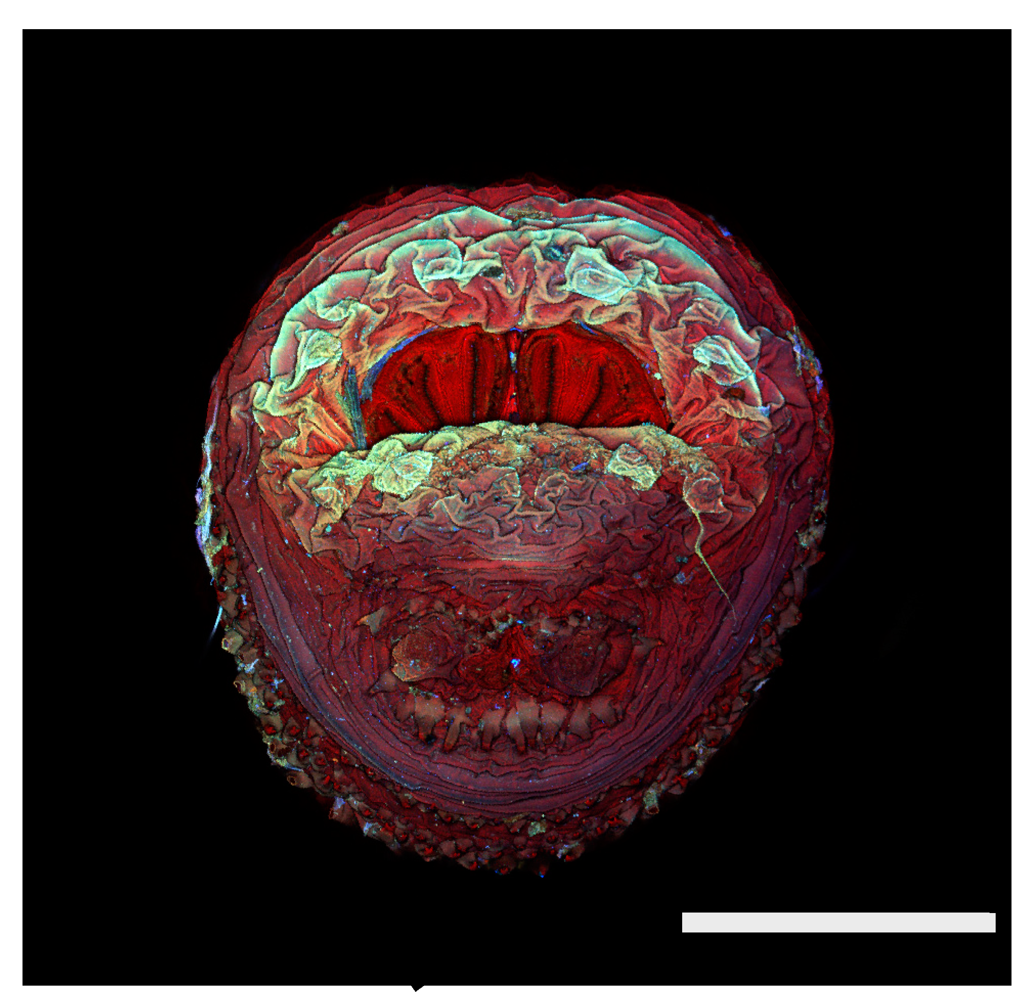
Figure 3.
Cochliomyia hominivorax puparium. Confocal maximum intensity projection at 40×, scale bar is 1 mm. Yellow polygon highlights spiracular labellum which obscures spiracular plates and spiracular opercula. SpS: spiracular slits; SpP: spiracular plate; AC: anal cleft.
Figure 3.
Cochliomyia hominivorax puparium. Confocal maximum intensity projection at 40×, scale bar is 1 mm. Yellow polygon highlights spiracular labellum which obscures spiracular plates and spiracular opercula. SpS: spiracular slits; SpP: spiracular plate; AC: anal cleft.
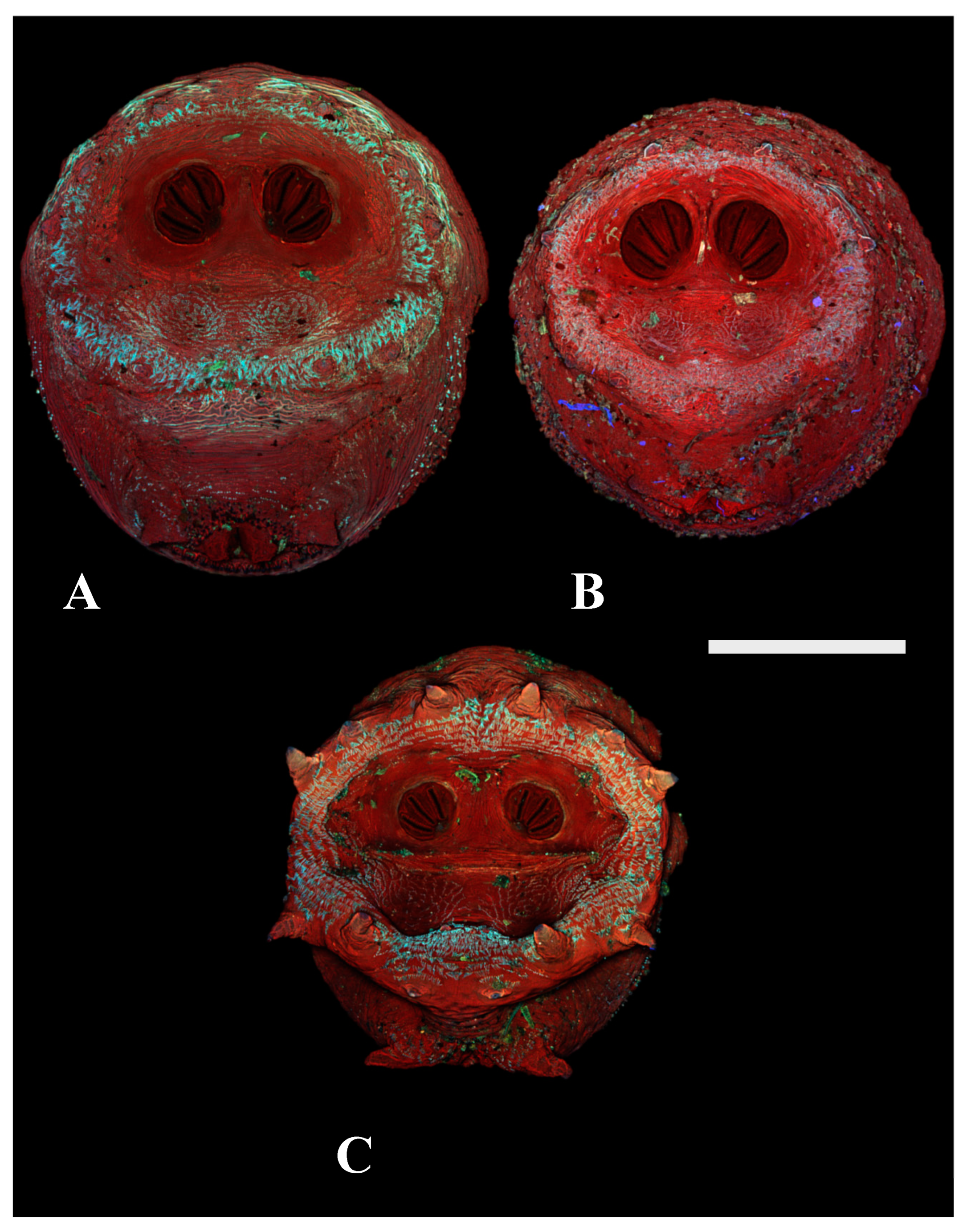
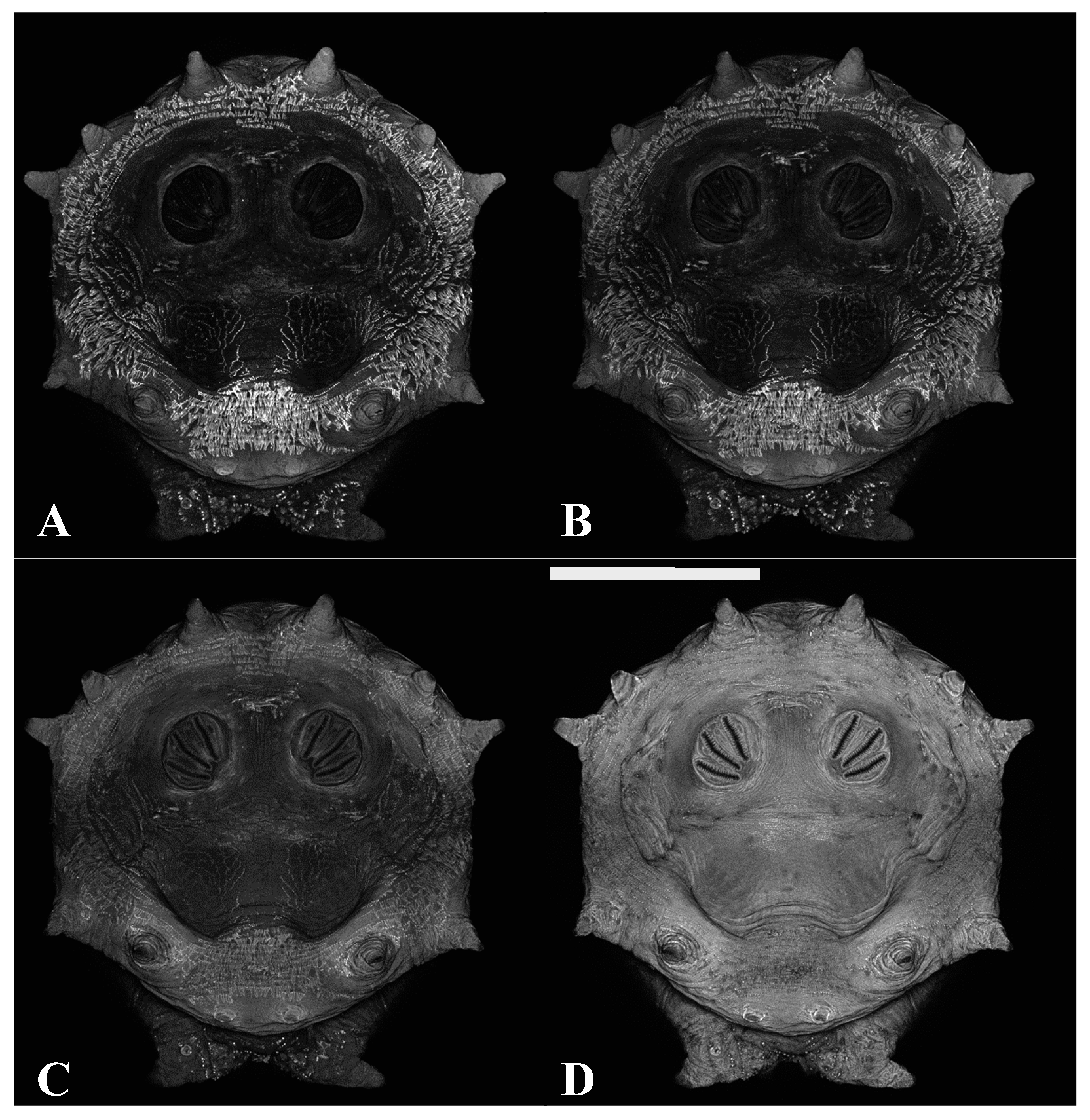
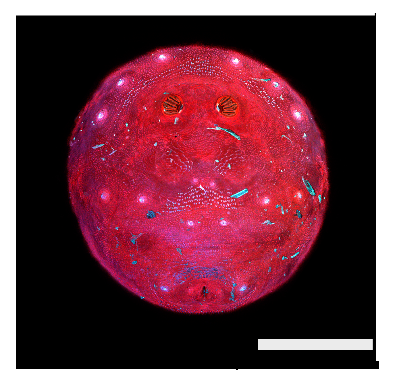
Figure 4.
Confocal maximum intensity projections of puparia at 40×, scale bar is 1 mm. (A) Chrysomya megacephala scored as a “0” for lacking prominent papillae. (B) Phormia regina scored as a “1” for presence of perispiracular papillae. (C) Protophormia terraenovae scored as a “2” with very prominent perispiracular papillae, in this case visible with the naked eye.
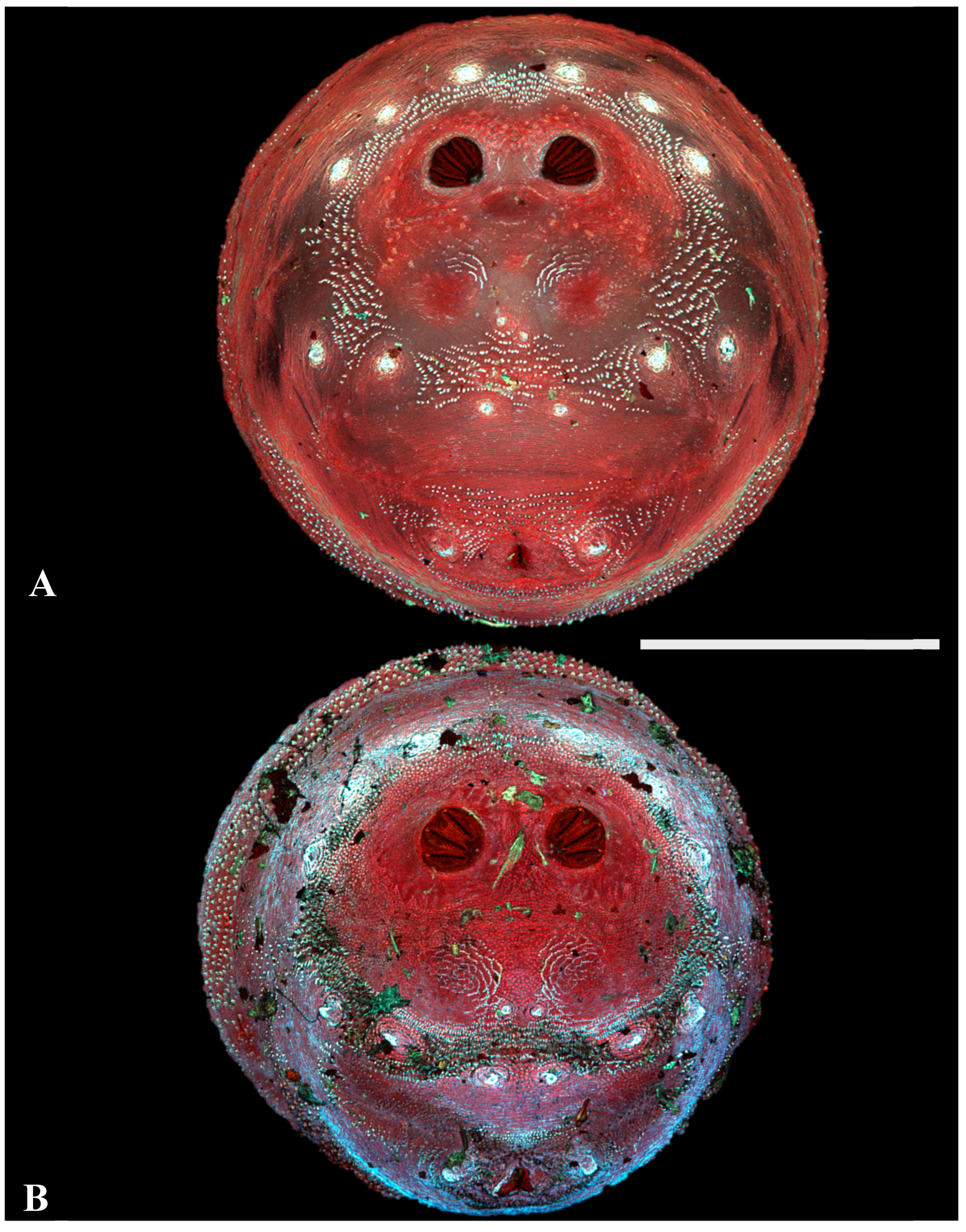
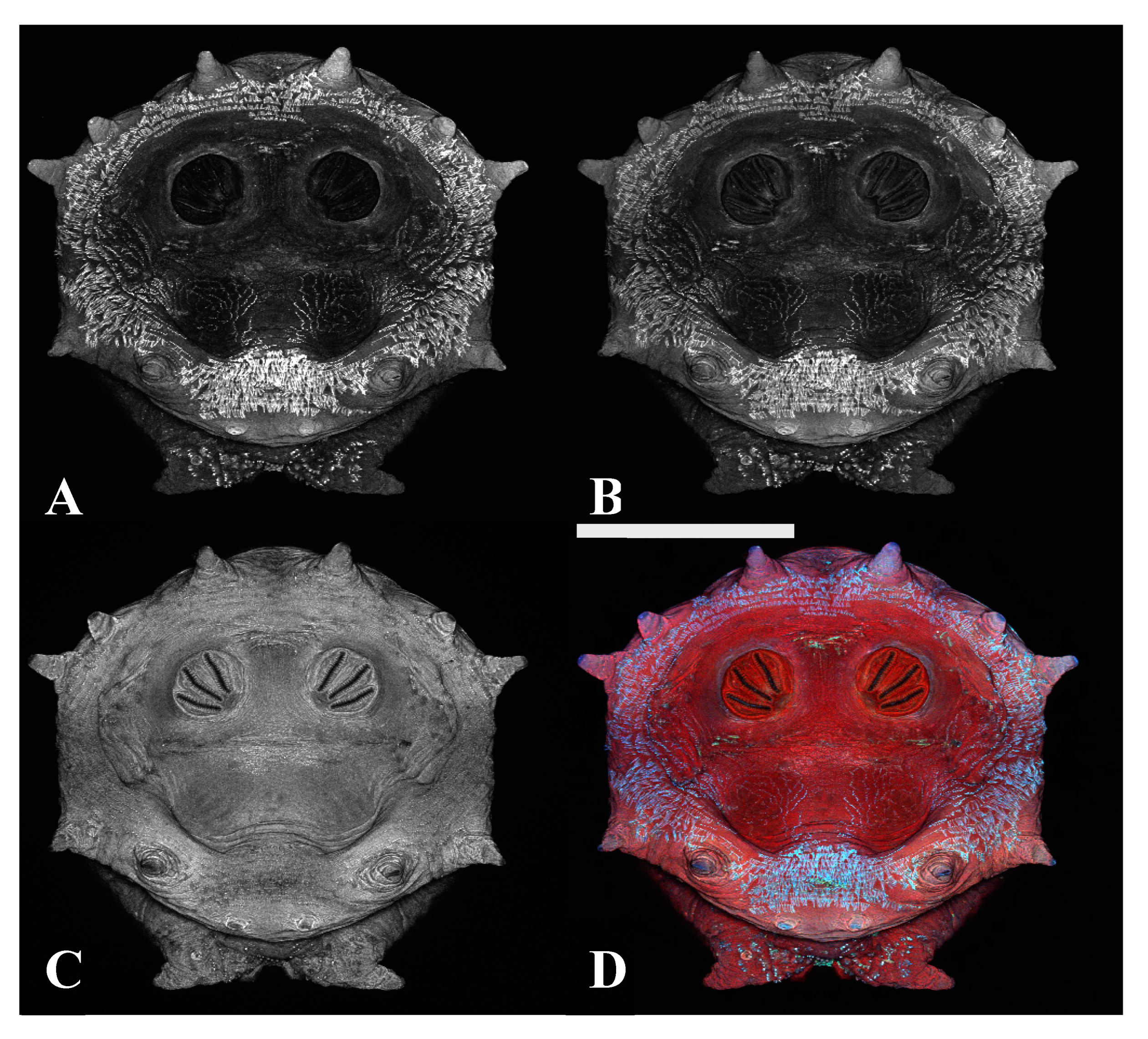
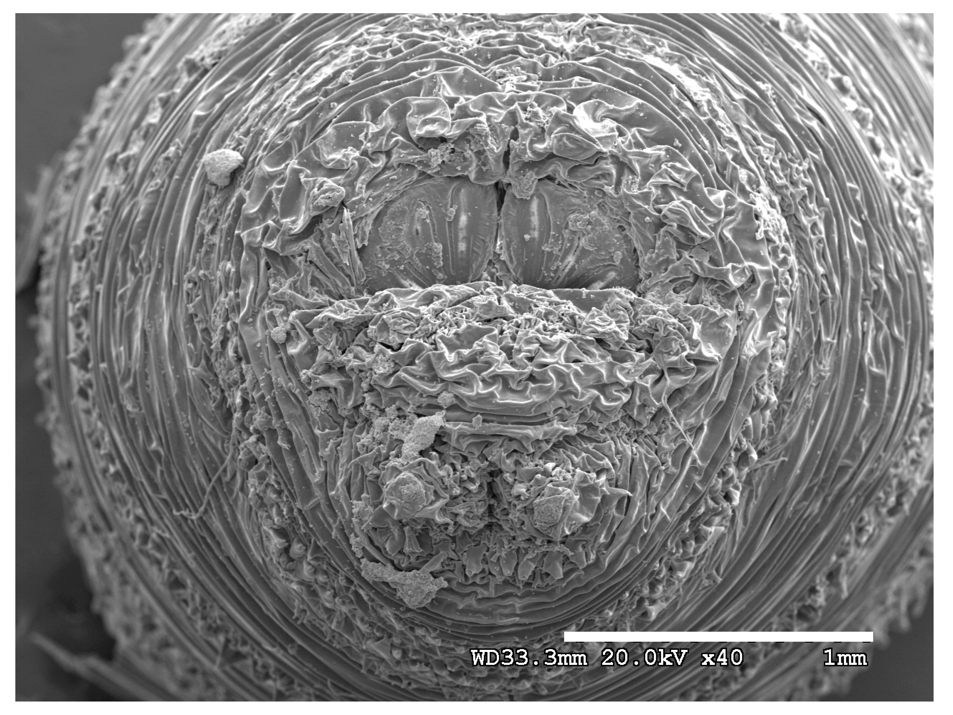
Figure 5.
Phormia regina puparia. Confocal maximum intensity projection at 40×, scale bar is 1 mm. Upper was scored as “1” for visible papillae, lower was scored at “0”. P: perispiracular papillae.
Figure 5.
Phormia regina puparia. Confocal maximum intensity projection at 40×, scale bar is 1 mm. Upper was scored as “1” for visible papillae, lower was scored at “0”. P: perispiracular papillae.
Figure 6.
Luciliinae. Confocal maximum intensity projections of puparia at 40×, scale bar is 1 mm. (A) Lucilia sericata; (B) L. coeruleiviridis.
Figure 6.
Luciliinae. Confocal maximum intensity projections of puparia at 40×, scale bar is 1 mm. (A) Lucilia sericata; (B) L. coeruleiviridis.
Figure 7.
Calliphorinae. Confocal maximum intensity projections of puparia at 40×, scale bar is 1 mm. (A) Calliphora livida, (B) Calliphora vicina, and (C) Cynomya cadaverina.
Figure 7.
Calliphorinae. Confocal maximum intensity projections of puparia at 40×, scale bar is 1 mm. (A) Calliphora livida, (B) Calliphora vicina, and (C) Cynomya cadaverina.
Figure 8.
Chrysomyinae. Confocal maximum intensity projections of puparia at 40×, scale bar is 1 mm. (A) Cochliomyia macellaria, (B) Cochliomyia hominivorax, (C) Phormia regina, (D) Chrysomya megacephala, and (E) Protophormia terraenovae.
Figure 8.
Chrysomyinae. Confocal maximum intensity projections of puparia at 40×, scale bar is 1 mm. (A) Cochliomyia macellaria, (B) Cochliomyia hominivorax, (C) Phormia regina, (D) Chrysomya megacephala, and (E) Protophormia terraenovae.
Figure 9.
Cochliomyia macellaria puparium, dissecting microscope. Dissecting microscope image at a total magnification of 40×. Spiracular plates with slits and spiracular opercula easily viewed at this minimal magnification. Note pigmented perianal spines (dentate setae), which appear dark.
Figure 9.
Cochliomyia macellaria puparium, dissecting microscope. Dissecting microscope image at a total magnification of 40×. Spiracular plates with slits and spiracular opercula easily viewed at this minimal magnification. Note pigmented perianal spines (dentate setae), which appear dark.
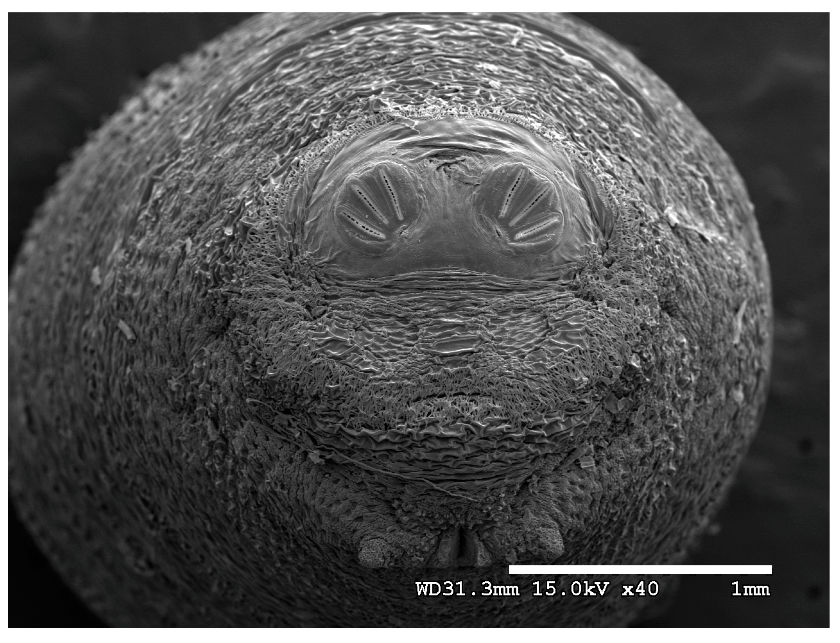
Figure 10.
Protophormia terraenovae puparium. Imaged sequentially with four excitation lasers with four emissions at 40×, scale bar is 1 mm. Data shown are a maximum intensity projection of all images. (A) The 404.7 nm excitation and data are 425–475 nm emission. (B) The 488 nm excitation and data are 500–550 nm emission. (C) The 561 nm excitation and data are 575–625 nm emission. (D) The 640.5 nm excitation and data are 663–738 nm emission. Autofluorescence is quite low in the 500–500 nm and 575–625 nm channels with sequential acquisition.
Figure 11.
Protophormia terraenovae puparium. Imaged with four excitation lasers with four emissions simultaneously at 40×, scale bar is 1 mm. Data shown are a maximum intensity projection of all images. (A) The 404.7 nm excitation and data are 425–475 nm emission. (B) The 488 nm excitation and data are 500–550 nm emission. (C) The 561 nm excitation and data are 575–625 nm emission. (D) The 640.5 nm excitation and data are 663–738 nm emission. (C) Contains similar data as three other channels, providing no contrast between signal areas.
Figure 12.
Protophormia terraenovae puparium. Imaged with three excitation lasers with three emissions simultaneously at 40×, scale bar is 1 mm. Data shown are a maximum intensity projection of all images. (A) The 404.7 nm excitation and 425–475 nm emission. (B) The 488 nm excitation and 500–550 nm emission. (C) The 640.5 nm excitation and 663–738 nm emission. (D) Merging of three datasets: A = blue, B = green, C = red.
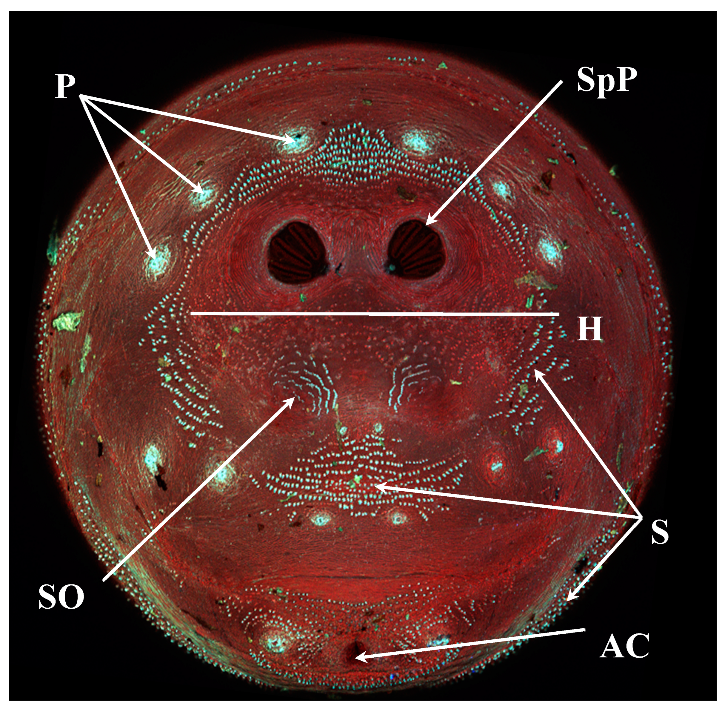
Figure 13.
Lucilia sericata puparium. P: papillae; SpP: spiracular plate; H: hinge; S: setae; SO: spiracular operculum; AC: anal cleft.
Figure 13.
Lucilia sericata puparium. P: papillae; SpP: spiracular plate; H: hinge; S: setae; SO: spiracular operculum; AC: anal cleft.
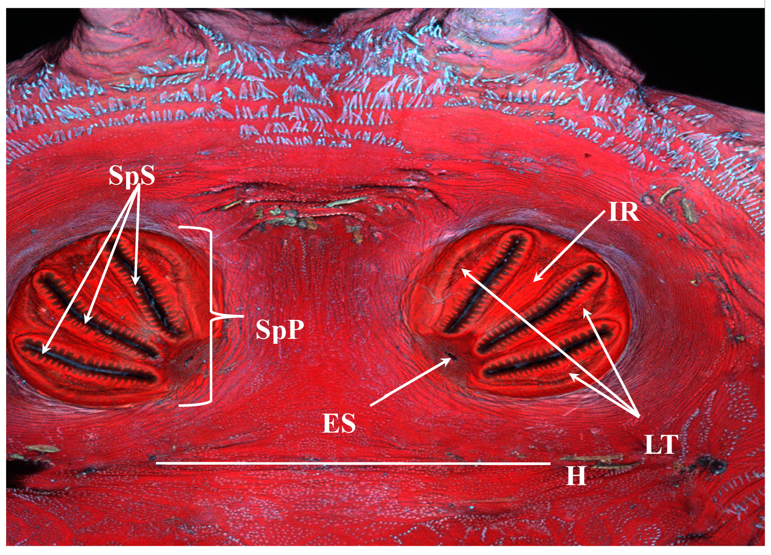
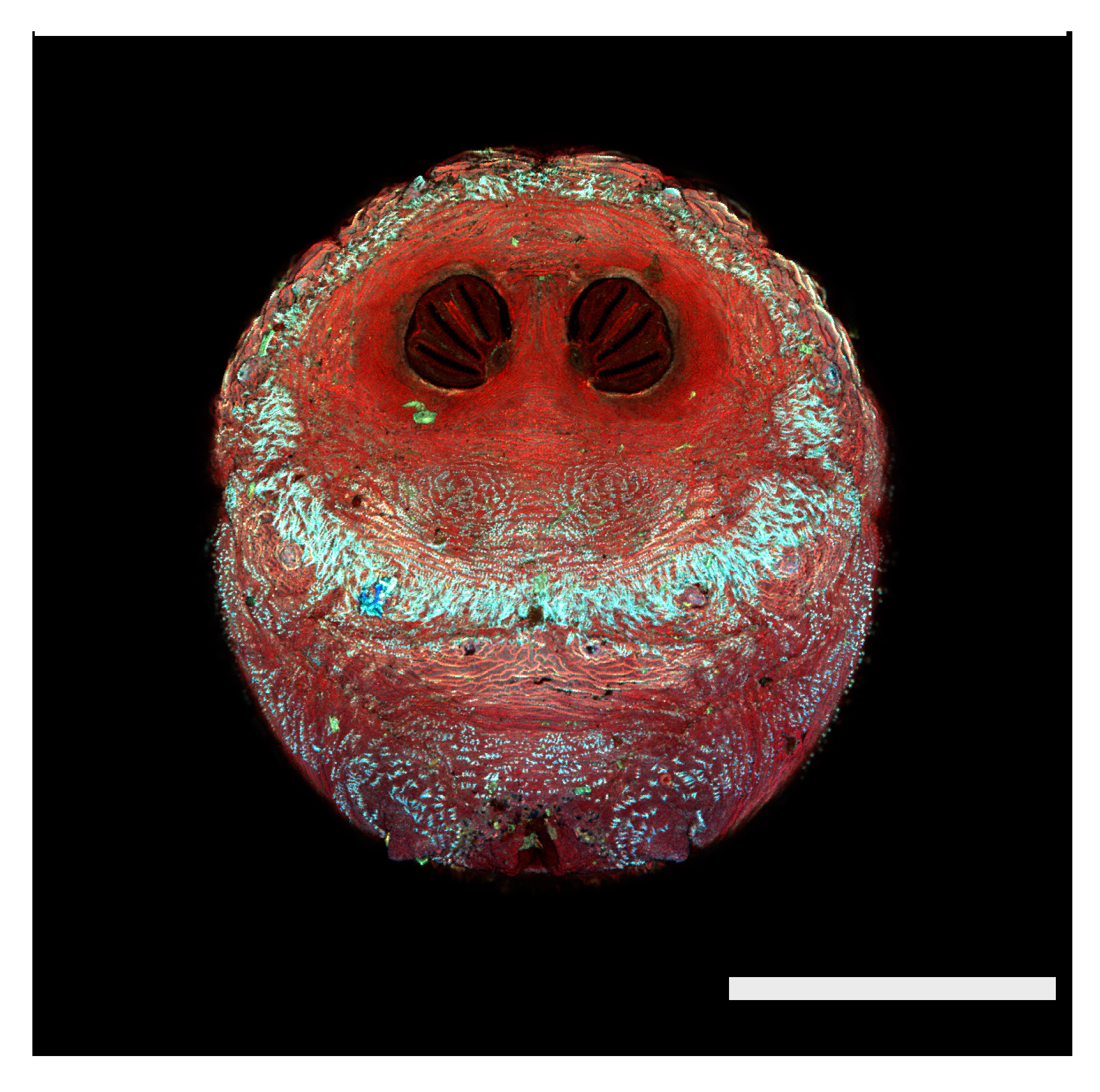
Figure 14.
Protophormia terraenovae puparium. Confocal maximum intensity projection. SpS: spiracular slits; SpP: spiracular plate; ES: ecdysial scar; LT: lateral thickenings; IR: intermediate ray; H: hinge.
Figure 14.
Protophormia terraenovae puparium. Confocal maximum intensity projection. SpS: spiracular slits; SpP: spiracular plate; ES: ecdysial scar; LT: lateral thickenings; IR: intermediate ray; H: hinge.
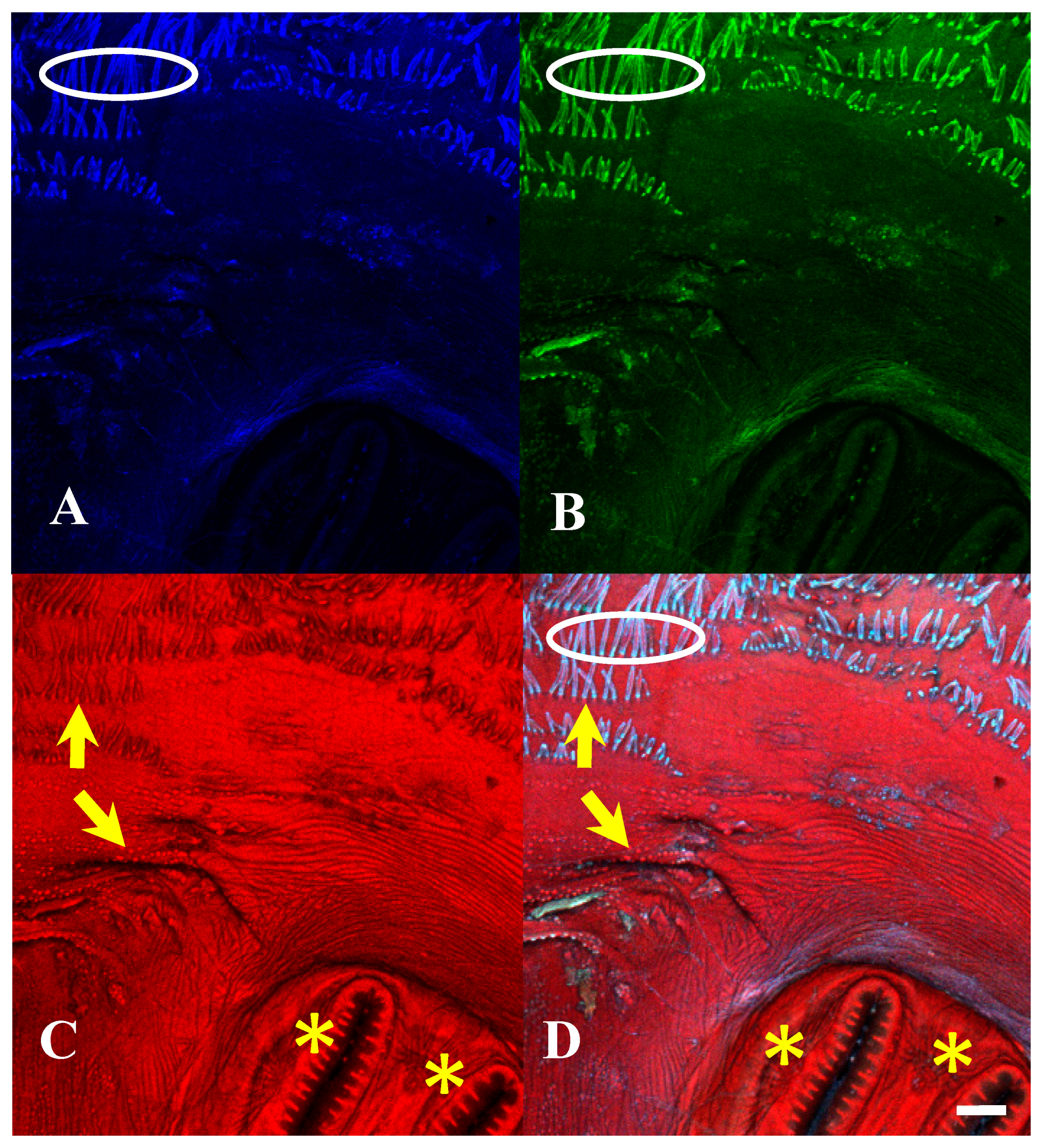
Figure 15.
Protophormia terraenovae puparium. Imaged with three excitation lasers with three emissions simultaneously at 100×, scale bar is 500 µm. (A) The 404.7 nm excitation and data are 425–475 nm emission. (B) The 488 nm excitation and data are 500–550 nm emission. (C) The 640.5 nm excitation and data are 663–738 nm emission. (D) Merge of all three datasets: (A) = blue, (B) = green, (C) = red. Yellow arrows in (C,D) indicate scleriterized structures; yellow * indicates “spiracular hair cluster”, which is not fluorescent but is slightly visible due to refraction of the signal from the other autofluorescence signals, sometimes found on slits and rays. White ovals in (A,B,D) indicate bright autofluorescence from hydrocarbons on setae.
Figure 16.
Cochliomyia macellaria puparium. Confocal maximum intensity projection at 40×, scale bar is 1 mm. Both samples came from the same cohort; the lower was an extremely lightly colored puparium, the upper more typical. Note that the spiracular plate and slit sizes are nearly identical. Blue and light green debris is easily differentiated from puparium.
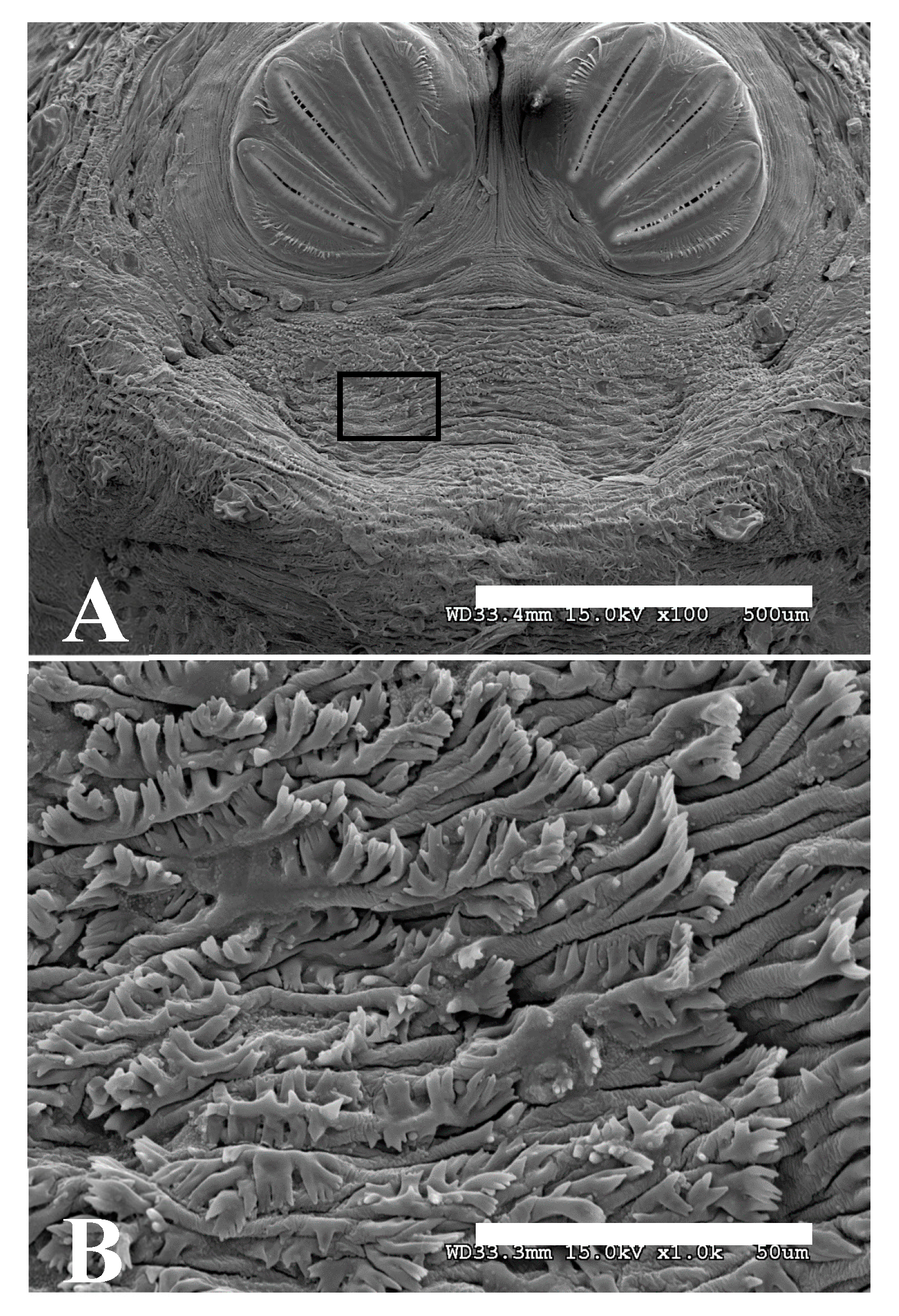
Figure 17.
Phormia regina puparium. (A) Scanning electron micrograph at 100×, scale bar is 500 µm. Black box is in a spiracular operculum and used as insert for (B). (B) Scanning electron micrograph at 1000× scale bar is 50 µm. Tips of setae which are covered in hydrocarbons are comb-like in appearance.
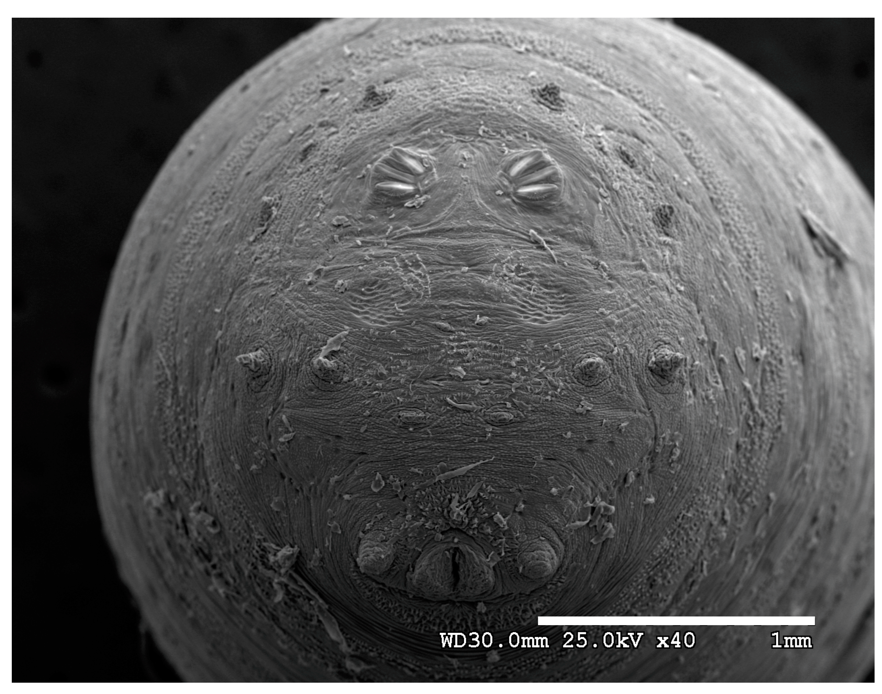
Figure 18.
Protophormia terraenovae puparium. Scanning electron micrograph at 40×, scale bar is 1 mm. Spiracular plates with slits are visible at this minimal magnification. Ecdysial scars are also visible. Prominent papillae are present in this species. Spiracular opercula are quite smooth but visible. “Spiracular hair cluster” visible bordering the spiracular slits. Intermediate rays are weakly visible here.
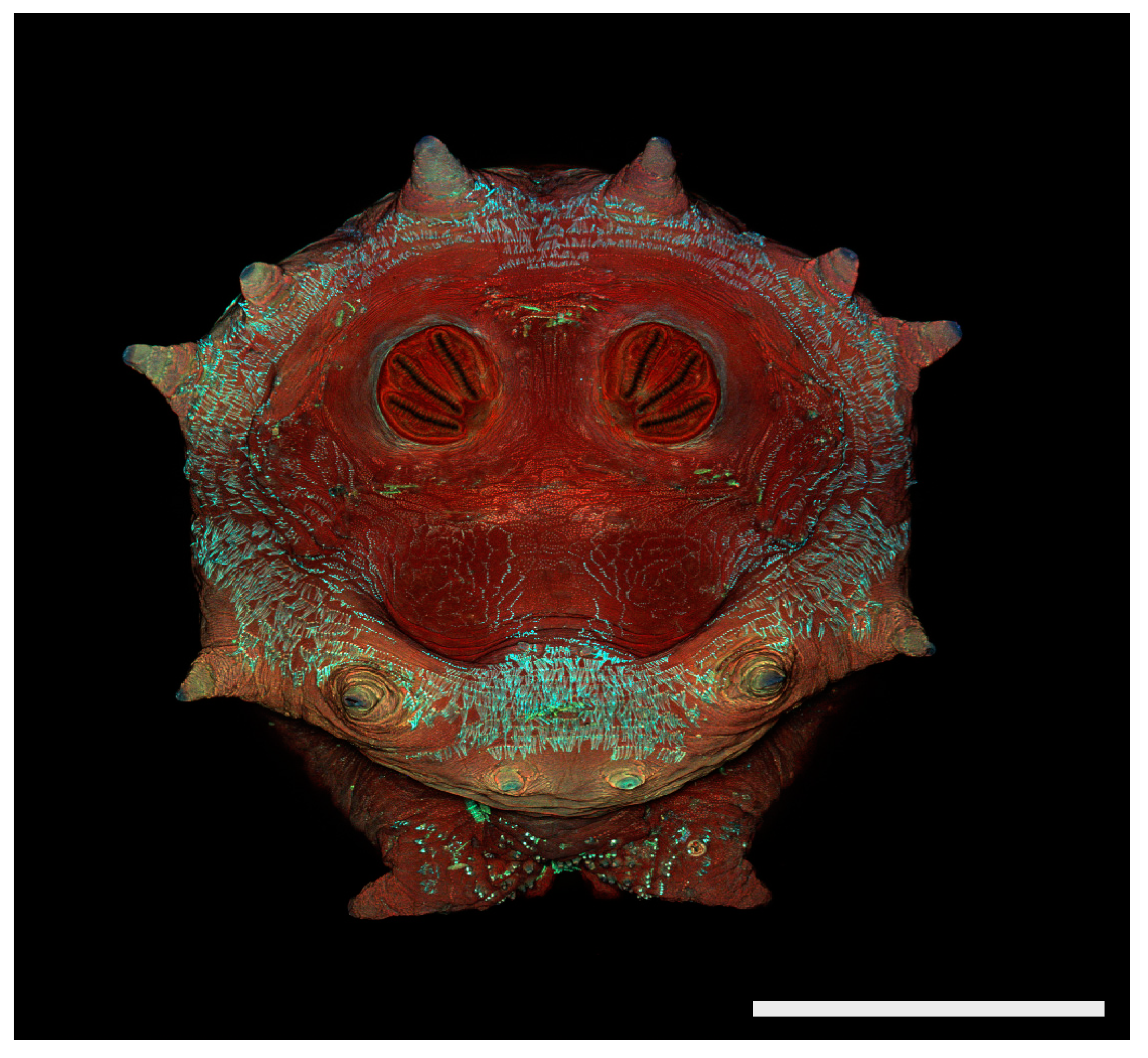
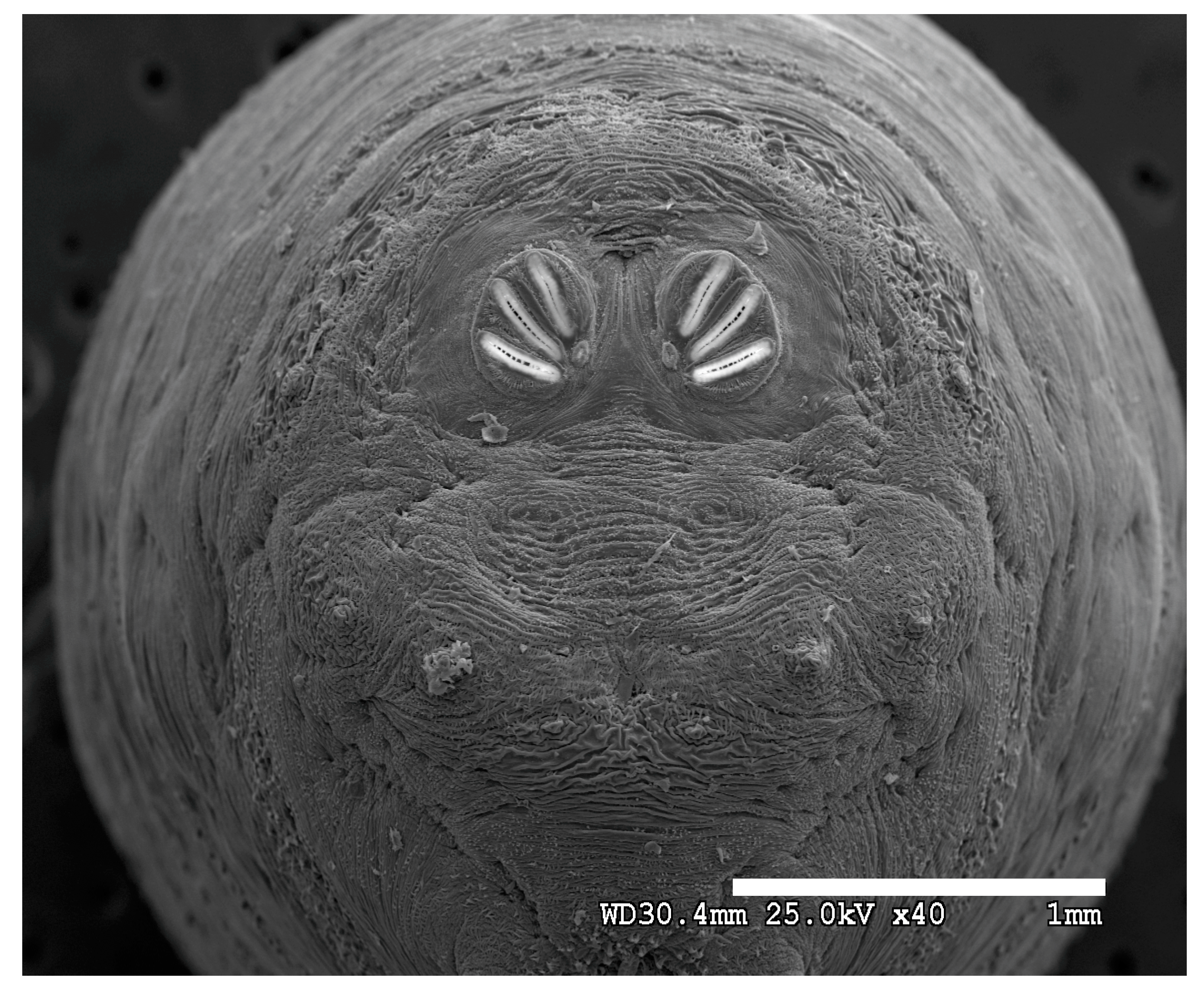
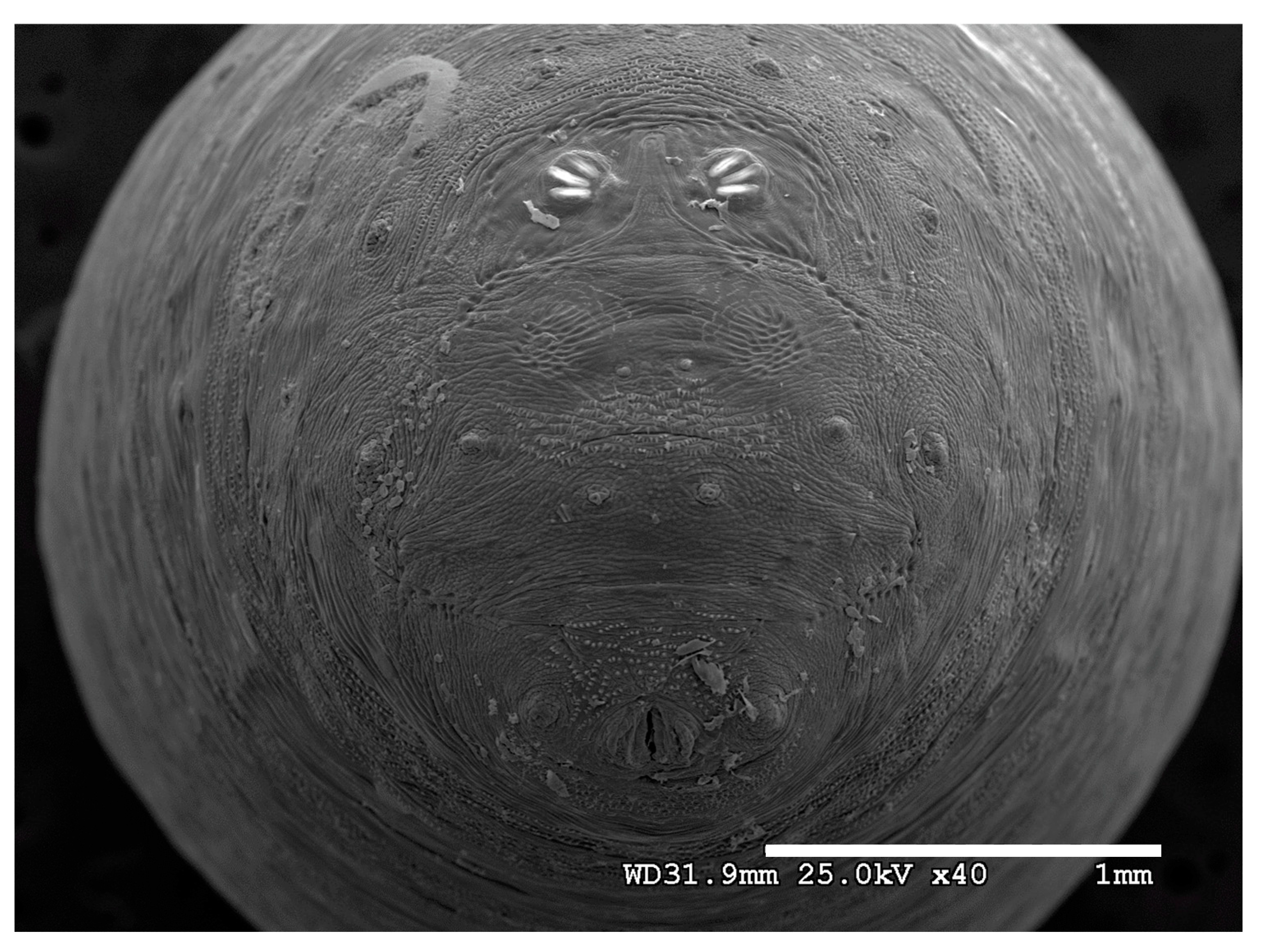
Figure 19.
Protophormia terraenovae puparium. Confocal maximum intensity projection at 40×, scale bar is 1 mm. Spiracular plates with slits and spiracular opercula are easily viewed at this minimal magnification due to contrasting coloration of structures. Intermediate rays are weakly visible here.
Figure 19.
Protophormia terraenovae puparium. Confocal maximum intensity projection at 40×, scale bar is 1 mm. Spiracular plates with slits and spiracular opercula are easily viewed at this minimal magnification due to contrasting coloration of structures. Intermediate rays are weakly visible here.
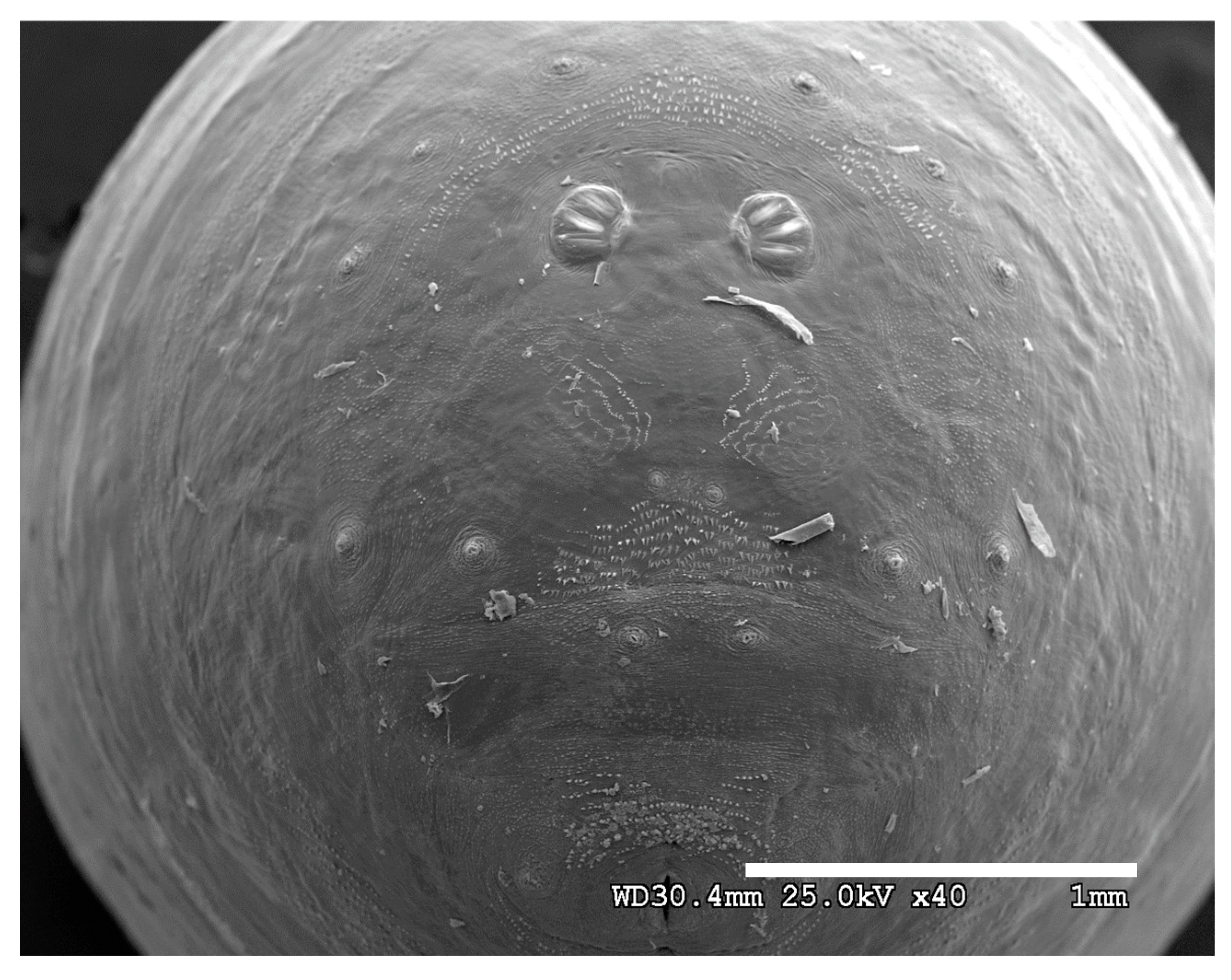
Figure 20.
Phormia regina puparium. Scanning electron micrograph at 40×, scale bar is 1 mm. Spiracular plates with slits and sunken and deeply sculptured spiracular opercula are easily viewed at this minimal magnification. Ecdysial scars are also visible. Papillae present.
Figure 20.
Phormia regina puparium. Scanning electron micrograph at 40×, scale bar is 1 mm. Spiracular plates with slits and sunken and deeply sculptured spiracular opercula are easily viewed at this minimal magnification. Ecdysial scars are also visible. Papillae present.
Figure 21.
Phormia regina puparium. Confocal maximum intensity projection at 40×, scale bar is 1 mm. Spiracular plates with slits and spiracular opercula are easily viewed at this minimal magnification.
Figure 21.
Phormia regina puparium. Confocal maximum intensity projection at 40×, scale bar is 1 mm. Spiracular plates with slits and spiracular opercula are easily viewed at this minimal magnification.
Figure 22.
Chrysomya megacephala puparium. Scanning electron micrograph at 40×, scale bar is 1 mm. Spiracular plates with slits and spiracular opercula are easily viewed at this minimal magnification. Ecdysial scars are also visible.
Figure 22.
Chrysomya megacephala puparium. Scanning electron micrograph at 40×, scale bar is 1 mm. Spiracular plates with slits and spiracular opercula are easily viewed at this minimal magnification. Ecdysial scars are also visible.
Figure 23.
Chrysomya megacephala puparium. Confocal maximum intensity projection at 40×, scale bar is 1 mm. Spiracular plates with slits and spiracular opercula are easily viewed at this minimal magnification. Ecdysial scars are also visible.
Figure 23.
Chrysomya megacephala puparium. Confocal maximum intensity projection at 40×, scale bar is 1 mm. Spiracular plates with slits and spiracular opercula are easily viewed at this minimal magnification. Ecdysial scars are also visible.
Figure 24.
Cochliomyia macellaria puparium. Scanning electron micrograph at 40×, scale bar is 1 mm. Spiracular plates with slits and spiracular opercula are easily viewed at this minimal magnification. Ecdysial scars are also visible.
Figure 24.
Cochliomyia macellaria puparium. Scanning electron micrograph at 40×, scale bar is 1 mm. Spiracular plates with slits and spiracular opercula are easily viewed at this minimal magnification. Ecdysial scars are also visible.
Figure 25.
Cochliomyia macellaria puparium. Confocal maximum intensity projection at 40×, scale bar is 1 mm. Spiracular plates with slits and spiracular opercula are easily viewed at this minimal magnification. Note pigmented perianal spines which appear dark. Ecdysial scars are also visible.
Figure 25.
Cochliomyia macellaria puparium. Confocal maximum intensity projection at 40×, scale bar is 1 mm. Spiracular plates with slits and spiracular opercula are easily viewed at this minimal magnification. Note pigmented perianal spines which appear dark. Ecdysial scars are also visible.
Figure 26.
Cochliomyia hominivorax puparium. Scanning electron micrograph at 40×, scale bar is 1 mm. Spiracular plates are partially covered by the spiracular labellum.
Figure 26.
Cochliomyia hominivorax puparium. Scanning electron micrograph at 40×, scale bar is 1 mm. Spiracular plates are partially covered by the spiracular labellum.
Figure 27.
Cochliomyia hominivorax puparium. Confocal maximum intensity projection at 40×, scale bar is 1 mm. Spiracular plates are partially covered by the spiracular labellum.
Figure 27.
Cochliomyia hominivorax puparium. Confocal maximum intensity projection at 40×, scale bar is 1 mm. Spiracular plates are partially covered by the spiracular labellum.
Figure 28.
Lucilia sericata puparium. Scanning electron micrograph at 40×, scale bar is 1 mm. Spiracular plates with slits and are easily viewed at this minimal magnification, but the spiracular opercula are weak.
Figure 28.
Lucilia sericata puparium. Scanning electron micrograph at 40×, scale bar is 1 mm. Spiracular plates with slits and are easily viewed at this minimal magnification, but the spiracular opercula are weak.
Figure 29.
Lucilia sericata puparium. Confocal maximum intensity projection at 40×, scale bar is 1 mm. Spiracular plates with slits and weak spiracular opercula are easily viewed at this minimal magnification.
Figure 29.
Lucilia sericata puparium. Confocal maximum intensity projection at 40×, scale bar is 1 mm. Spiracular plates with slits and weak spiracular opercula are easily viewed at this minimal magnification.
Figure 30.
Lucilia coeruleiviridis puparium. Scanning electron micrograph at 40×, scale bar is 1 mm. Spiracular plates with slits easily viewed at this minimal magnification. Spiracular opercula difficult to distinguish.
Figure 30.
Lucilia coeruleiviridis puparium. Scanning electron micrograph at 40×, scale bar is 1 mm. Spiracular plates with slits easily viewed at this minimal magnification. Spiracular opercula difficult to distinguish.
Figure 31.
Lucilia coeruleiviridis puparium. Confocal maximum intensity projection at 40×, scale bar is 1 mm. Spiracular plates with slits and spiracular opercula are easily viewed at this minimal magnification. While weak, setae of the spiracular opercula are more robust than in L. sericata.
Figure 31.
Lucilia coeruleiviridis puparium. Confocal maximum intensity projection at 40×, scale bar is 1 mm. Spiracular plates with slits and spiracular opercula are easily viewed at this minimal magnification. While weak, setae of the spiracular opercula are more robust than in L. sericata.
Figure 32.
Cynomya cadaverina puparium. Scanning electron micrograph at 40×, scale bar is 1 mm. Spiracular plates with slits and spiracular opercula are easily viewed at this minimal magnification. Ecdysial scars are also visible.
Figure 32.
Cynomya cadaverina puparium. Scanning electron micrograph at 40×, scale bar is 1 mm. Spiracular plates with slits and spiracular opercula are easily viewed at this minimal magnification. Ecdysial scars are also visible.
Figure 33.
Cynomya cadaverina puparium. Confocal maximum intensity projection at 40×, scale bar is 1 mm. Spiracular plates with slits and spiracular opercula are easily viewed at this minimal magnification.
Figure 33.
Cynomya cadaverina puparium. Confocal maximum intensity projection at 40×, scale bar is 1 mm. Spiracular plates with slits and spiracular opercula are easily viewed at this minimal magnification.
Figure 34.
Calliphora livida puparium. Scanning electron micrograph at 40×, scale bar is 1 mm. Setae of the spiracular opercula are weak.
Figure 34.
Calliphora livida puparium. Scanning electron micrograph at 40×, scale bar is 1 mm. Setae of the spiracular opercula are weak.
Figure 35.
Calliphora livida puparium. Confocal maximum intensity projection at 40×, scale bar is 1 mm. Spiracular plates with slits and spiracular opercula are easily viewed at this minimal magnification.
Figure 35.
Calliphora livida puparium. Confocal maximum intensity projection at 40×, scale bar is 1 mm. Spiracular plates with slits and spiracular opercula are easily viewed at this minimal magnification.
Figure 36.
Calliphora vicina puparium. Scanning electron micrograph at 40×, scale bar is 1 mm. Spiracular plates with slits and spiracular opercula are easily viewed at this minimal magnification. Ecdysial scars are also visible.
Figure 36.
Calliphora vicina puparium. Scanning electron micrograph at 40×, scale bar is 1 mm. Spiracular plates with slits and spiracular opercula are easily viewed at this minimal magnification. Ecdysial scars are also visible.
Figure 37.
Calliphora vicina puparium. Confocal maximum intensity projection at 40×, scale bar is 1 mm. Spiracular plates with slits and spiracular opercula are easily viewed at this minimal magnification.
Figure 37.
Calliphora vicina puparium. Confocal maximum intensity projection at 40×, scale bar is 1 mm. Spiracular plates with slits and spiracular opercula are easily viewed at this minimal magnification.
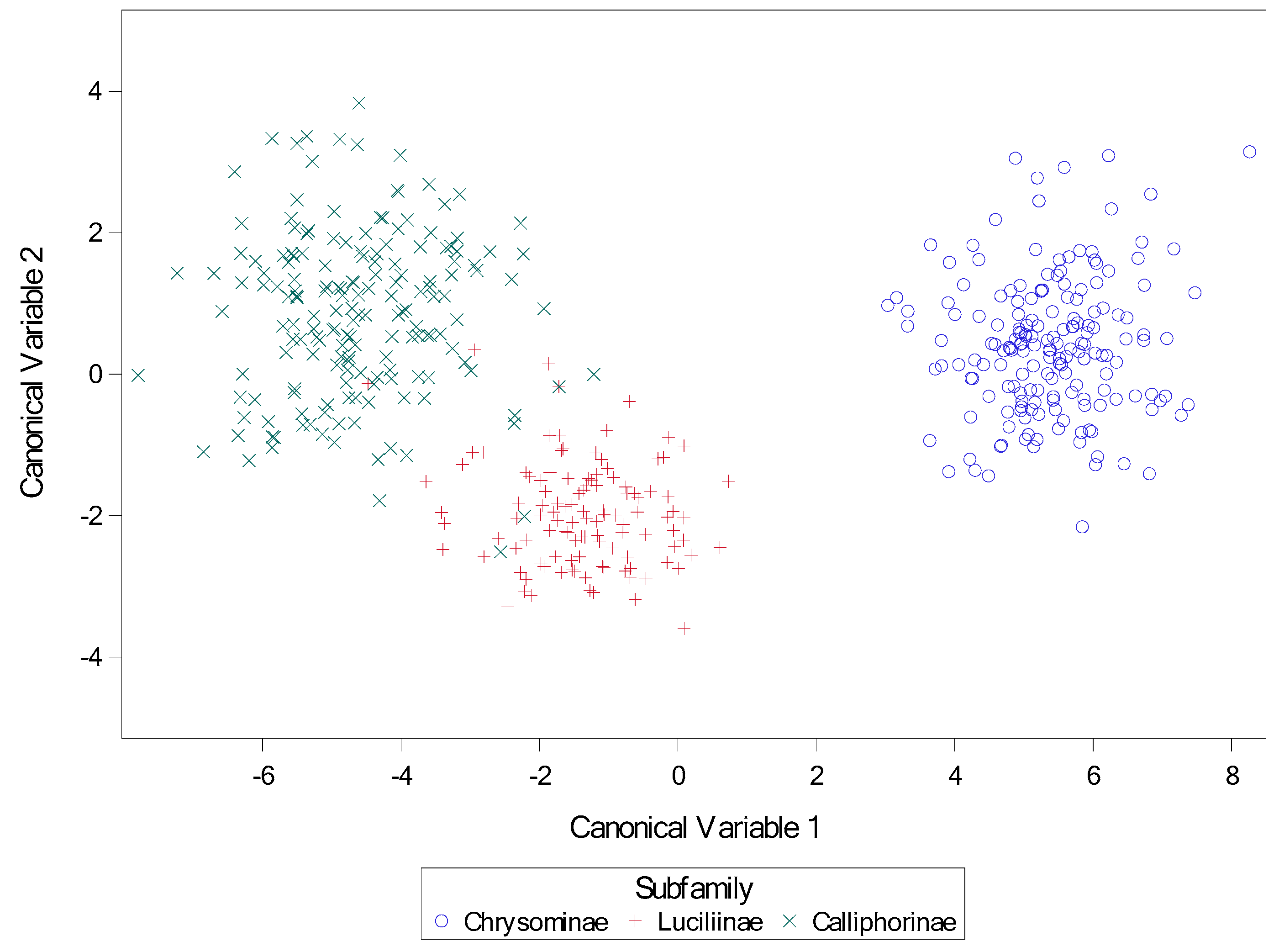
Figure 38.
Scatter plot of canonical variates for subfamily. Canonical variables 1 and 2 from canonical discriminate analysis across nine calliphorid species for subfamily. Variables for canonical analysis (based on results from stepwise discriminate analysis) were length2 = the length of the middle slit of the left spiracular plate, angle4 = the angle of the middle slit of the right spiracular plate, and narrow = the narrowest length between plates.
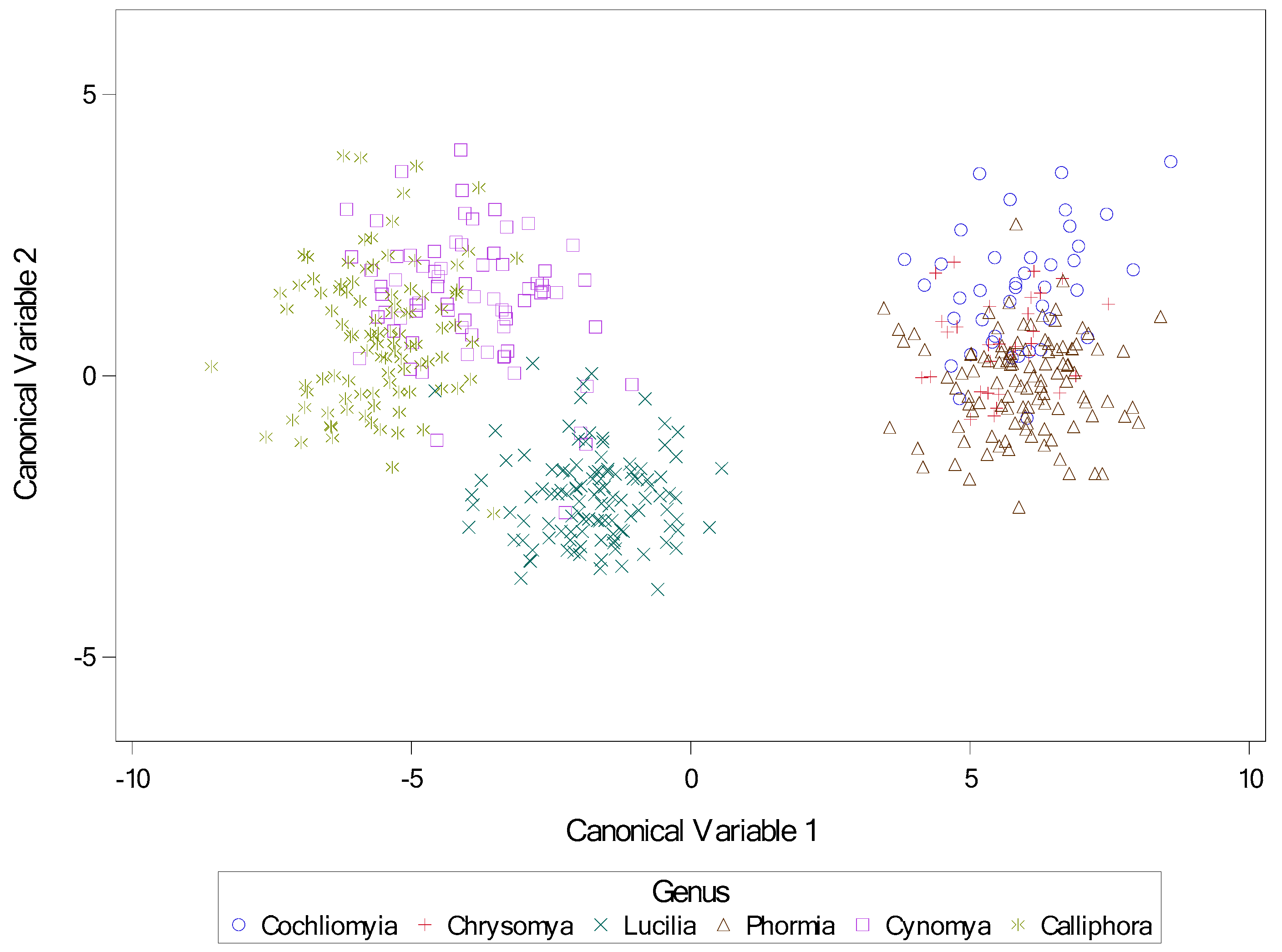
Figure 39.
Scatter plot of canonical variables for genus. Canonical variables1 and 2 from canonical discriminate analysis across nine calliphorid species by genus. Variables for canonical analysis (based on results from stepwise discriminate analysis) were length2 = the length of the middle slit of the left spiracular plate, angle4 = the angle of the middle slit of the right spiracular plate, and narrow = the narrowest length between plates.
Figure 40.
Scatter plot of canonical variables by species. Canonical variables 1 and 2 from canonical discriminate analysis across nine calliphorid species. Variables for canonical analysis (based on results from stepwise discriminate analysis) were length2 = the length of the middle slit of the left spiracular plate, angle4 = the angle of the middle slit of the right spiracular plate, and narrow = the narrowest length between plates.
Table 1.
Background data on specimens. Taxonomic information, number of specimens imaged, location, sources, and diet of calliphorid larvae. A total of 505 individuals were used.
Table 1.
Background data on specimens. Taxonomic information, number of specimens imaged, location, sources, and diet of calliphorid larvae. A total of 505 individuals were used.
| Subfamily | Genus | Species | n | Location | Source | Host/Food |
|---|
| Calliphorinae | Calliphora | livida | 21 | Everett, WA, USA | wild | rat |
| Calliphorinae | Calliphora | vicina | 20 | Everett, WA, USA | wild | rat |
| Calliphorinae | Calliphora | vicina | 57 | Everett, WA, USA | wild | rat |
| Chrysomyinae | Chrysomya | megacephala | 30 | Miami, FL, USA | wild | chicken |
| Chrysomyinae | Cochliomyia | hominivorax | 11 | Pacora, Panama 1 | culture | artificial diet |
| Chrysomyinae | Cochliomyia | macellaria | 40 | Lincoln, NE, USA | wild | pig |
| Calliphorinae | Cynomya | cadaverina | 76 | Lincoln, NE, USA | wild | raccoon |
| Luciliinae | Lucilia | coeruleiviridis | 14 | Lincoln, NE, USA | wild | rabbit |
| Luciliinae | Lucilia | sericata | 35 | Lincoln, NE, USA 2 | culture | beef liver |
| Luciliinae | Lucilia | sericata | 64 | Lincoln, NE, USA | wild | rat |
| Chrysominae | Phormia | regina | 39 | Lincoln, NE, USA | wild | pig |
| Chrysominae | Phormia | regina | 28 | Everett, WA, USA | wild | rat |
| Chrysominae | Phormia | regina | 39 | Lincoln, NE, USA | culture | beef liver |
| Chrysominae | Phormia | terraenovae | 31 | Bonners Ferry, ID, USA 3 | culture | fish meal |
Table 2.
Descriptive statistics for variables used for discrimination by subfamily of calliphorid. Variables are length2 = the length of the middle slit of the left spiracluar plate, angle4 = the angle of the middle slit of the right spiracular plate, and narrow = the narrowest length between plates.
| Subfamily | | Length2 | Angle4 | Narrow |
|---|
| Calliphorinae | N | 174 | 174 | 174 |
| Mean | 42.42563 | 36.81741 | 109.8691 |
| StdErr | 0.603716 | 0.396177 | 1.018223 |
| Chrysomyinae | N | 178 | 207 | 207 |
| Mean | 77.45124 | 65.80676 | 98.11097 |
| StdErr | 0.359465 | 0.372499 | 1.251904 |
| Luciliinae | N | 113 | 113 | 113 |
| Mean | 45.28814 | 49.99319 | 75.27035 |
| StdErr | 0.401046 | 0.452896 | 0.868647 |
Table 3.
Summary results from stepwise canonical discriminate analysis of morphological variables for distinguishing subfamilies of calliphorids (specifically, Calliphorinae, Chrysominae, and Luciliinae). Here, a significant F value indicates that the variable cannot be removed from the model (df = 2, 460). Variables are length2 = the length of the middle slit of the left spiracular plate, angle4 = the angle of the middle slit of the right spiracular plate, and narrow = the narrowest length between plates.
| Step | Variable | Partial
R-Square | F | p > F | Wilks’
Lambda | p < Lambda | Average
Squared
Canonical
Correlation | p > ASCC |
|---|
| 1 | length2 | 0.8813 | 1715.20 | <0.0001 | 0.10439509 | <0.0001 | 0.44780246 | <0.0001 |
| 2 | angle4 | 0.6692 | 466.30 | <0.0001 | 0.04189724 | <0.0001 | 0.65483543 | <0.0001 |
| 3 | narrow | 0.4617 | 197.29 | <0.0001 | 0.02771094 | <0.0001 | 0.75597814 | <0.0001 |
Table 4.
Summary univariate test statistics for canonical discriminate analysis of morphological variables for distinguishing subfamilies of calliphorids (specifically, Calliphorinae, Chrysomyinae, and Luciliinae). Variables are length2 = the length of the middle slit of the left spiracular plate, angle4 = the angle of the middle slit of the right spiracular plate, and narrow = the narrowest length between plates.
| Variable | Total
Standard
Deviation | Pooled
Standard
Deviation | Between
Standard
Deviation | R-Square | R-Square
/(1-RSq) | F2,462 | p > F |
|---|
| length2 | 17.6095 | 6.0799 | 20.2250 | 0.8813 | 7.4251 | 1715.20 | <0.0001 |
| angle4 | 13.9182 | 5.0221 | 15.8859 | 0.8704 | 6.7138 | 1550.89 | <0.0001 |
| narrow | 19.1516 | 13.7813 | 16.3078 | 0.4844 | 0.9396 | 217.04 | <0.0001 |
Table 5.
Summary multivariate test statistics and F approximations (S = 0, M = 0, and N = 229) for canonical discriminate analysis of morphological variables for distinguishing subfamilies of calliphorids (specifically Calliphorinae, Chrysomyinae, and Luciliinae).
Table 5.
Summary multivariate test statistics and F approximations (S = 0, M = 0, and N = 229) for canonical discriminate analysis of morphological variables for distinguishing subfamilies of calliphorids (specifically Calliphorinae, Chrysomyinae, and Luciliinae).
| Statistic | Value | F | Num DF | Den DF | p > F |
|---|
| Wilks’ Lambda | 0.02113448 | 901.40 | 6 | 920 | <0.0001 |
| Pillai’s Trace | 1.51598239 | 481.30 | 6 | 922 | <0.0001 |
| Hotelling–Lawley Trace | 20.90179552 | 1600.74 | 6 | 611.56 | <0.0001 |
| Roy’s Greatest Root | 19.60551526 | 3012.71 | 3 | 461 | <0.0001 |
Table 6.
Raw canonical coefficients for Can1 and Can2, which were used in separating calliphorid subfamilies of calliphorids (Calliphorinae, Chrysominae, and Luciliinae). Variables are length2 = the length of the middle slit of the left spiracular plate, angle4 = the angle of the middle slit of the right spiracular plate, and narrow = the narrowest length between plates.
| Variable | Can1 | Can2 |
|---|
| length2 | 0.1342688860 | 0.0709503297 |
| angle4 | 0.1677950339 | −0.0660280512 |
| narrow | −0.0186688625 | 0.0627152758 |
Table 7.
Descriptive statistics for variables used for discrimination by select genera of calliphorids (Calliphora, Chrysomya, Cochliomyia, Cynomya, Lucilia, and Phormia). Variables are length2 = the length of the middle slit of the left spiracular plate, angle4 = the angle of the middle slit of the right spiracular plate, and narrow = the narrowest length between plates.
| | Length2 | Angle4 | Narrow |
|---|
| Calliphora | N | 98 | 98 | 98 |
| Mean | 37.07776 | 38.56643 | 111.8896 |
| StdErr | 0.53704 | 0.51058 | 1.326149 |
| Chrysomya | N | 30 | 30 | 30 |
| Mean | 77.118 | 65.11933 | 96.118 |
| StdErr | 0.716633 | 0.935825 | 1.731377 |
| Cochliomyia | N | 40 | 40 | 40 |
| Mean | 76.12175 | 71.294 | 115.1433 |
| StdErr | 0.90666 | 0.639532 | 1.992577 |
| Cynomya | N | 76 | 76 | 76 |
| Mean | 49.32158 | 34.56211 | 107.2638 |
| StdErr | 0.563951 | 0.523184 | 1.543251 |
| Lucilia | N | 113 | 113 | 113 |
| Mean | 45.28814 | 49.99319 | 75.27035 |
| StdErr | 0.401046 | 0.452896 | 0.868647 |
| Phormia | N | 108 | 108 | 108 |
| Mean | 78.0362 | 65.23676 | 86.01204 |
| StdErr | 0.439375 | 0.392917 | 1.072371 |
Table 8.
Summary results from stepwise canonical discriminate analysis of morphological variables for distinguishing genera of calliphorids (specifically, Calliphora, Chrysomya, Cochliomyia, Cynomya, Lucilia, and Phormia). Here, a significant F value indicates that the variable cannot be removed from the model (df = 5, 457). Variables are length2 = the length of the middle slit of the left spiracular plate, angle4 = the angle of the middle slit of the right spiracular plate, and narrow = the narrowest length between plates.
| Step | Variable | Partial
R-Square | F | p > F | Wilks’
Lambda | p < Lambda | Average
Squared
Canonical
Correlation | p > ASCC |
|---|
| 1 | length2 | 0.9267 | 1160.18 | <0.0001 | 0.07332386 | <0.0001 | 0.18533523 | <0.0001 |
| 2 | angle4 | 0.7059 | 219.88 | <0.0001 | 0.02156298 | <0.0001 | 0.29147732 | <0.0001 |
| 3 | narrow | 0.6135 | 145.10 | <0.0001 | 0.00833359 | <0.0001 | 0.40665025 | <0.0001 |
Table 9.
Summary univariate test statistics for canonical discriminate analysis of morphological variables for distinguishing genera of calliphorids (specifically, Calliphora, Chrysomya, Cochliomyia, Cynomya, Lucilia, and Phormia). Variables are length2 = the length of the middle slit of the left spiracular plate, angle4 = the angle of the middle slit of the right spiracular plate, and narrow = the narrowest length between plates.
| Variable | Total
Standard
Deviation | Pooled
Standard
Deviation | Between
Standard
Deviation | R-Square | R-Square
/(1-RSq) | F5,459 | p > F |
|---|
| length2 | 17.6095 | 4.7943 | 18.5496 | 0.9267 | 12.6381 | 1160.18 | <0.0001 |
| angle4 | 13.9182 | 4.6250 | 14.3744 | 0.8908 | 8.1548 | 748.61 | <0.0001 |
| narrow | 19.1516 | 11.6160 | 16.7142 | 0.6361 | 1.7479 | 160.46 | <0.0001 |
Table 10.
Summary multivariate test statistics and F approximations (S = 3, M = 0.5, and N = 227.5) for canonical discriminate analysis of morphological variables for distinguishing genera of calliphorids (specifically, Calliphora, Chrysomya, Cochliomyia, Cynomya, Lucilia, and Phormia).
Table 10.
Summary multivariate test statistics and F approximations (S = 3, M = 0.5, and N = 227.5) for canonical discriminate analysis of morphological variables for distinguishing genera of calliphorids (specifically, Calliphora, Chrysomya, Cochliomyia, Cynomya, Lucilia, and Phormia).
| Statistic | Value | F | Num DF | Den DF | p > F |
|---|
| Wilks’ Lambda | 0.00833359 | 392.44 | 15 | 1262 | <0.0001 |
| Pillai’s Trace | 2.03325124 | 193.07 | 15 | 1377 | <0.0001 |
| Hotelling–Lawley Trace | 25.95452800 | 789.13 | 15 | 858 | <0.0001 |
| Roy’s Greatest Root | 23.40209892 | 2148.31 | 5 | 459 | <0.0001 |
Table 11.
Raw canonical coefficients for Can1 and Can2, which were used in separating genera of calliphorids (specifically, Calliphora, Chrysomya, Cochliomyia, Cynomya, Lucilia, I and Phormia). Variables are length2 = the length of the middle slit of the left spiracular plate, angle4 = the angle of the middle slit of the right spiracular plate, and narrow = the narrowest length between plates.
| Variable | Can1 | Can2 |
|---|
| length2 | 0.1741020171 | 0.0636367228 |
| angle4 | 0.1454001990 | −0.0571248148 |
| narrow | −0.0208380554 | 0.0743470086 |
Table 12.
Descriptive statistics for variables used for discrimination of eight species of calliphorids. Variables are length2 = the length of the middle slit of the left spiracular plate, angle4 = the angle of the middle slit of the right spiracular plate, and narrow = the narrowest length between plates.
| Species | | Length2 | Angle4 | Narrow |
|---|
| Calliphora livida | N | 21 | 21 | 21 |
| Mean | 33.41 | 37.37238 | 98.51238 |
| StdErr | 0.671428 | 0.867152 | 1.663625 |
| Calliphora vicina | N | 77 | 77 | 77 |
| Mean | 38.07805 | 38.89208 | 115.5379 |
| StdErr | 0.612128 | 0.602485 | 1.35678 |
| Chrysomya megacephala | N | 30 | 30 | 30 |
| Mean | 77.118 | 65.11933 | 96.118 |
| StdErr | 0.716633 | 0.935825 | 1.731377 |
| Cochliomya macellaria | N | 40 | 40 | 40 |
| Mean | 76.12175 | 71.294 | 115.1433 |
| StdErr | 0.90666 | 0.639532 | 1.992577 |
| Cynomya cadaverina | N | 76 | 76 | 76 |
| Mean | 49.32158 | 34.56211 | 107.2638 |
| StdErr | 0.563951 | 0.523184 | 1.543251 |
| Lucilia coeruleivirdis | N | 14 | 14 | 14 |
| Mean | 46.20071 | 46.13857 | 85.63643 |
| StdErr | 1.409753 | 1.914886 | 3.311618 |
| Lucilia sericata | N | 99 | 99 | 99 |
| Mean | 45.15909 | 50.53828 | 73.80444 |
| StdErr | 0.413709 | 0.417504 | 0.775613 |
| Phormia regina | N | 108 | 108 | 108 |
| Mean | 78.0362 | 65.23676 | 86.01204 |
| StdErr | 0.439375 | 0.392917 | 1.072371 |
Table 13.
Summary results from stepwise canonical discriminate analysis of morphological variables for distinguishing eight species of calliphorids (see text for list). Here, a significant F value indicates that the variable cannot be removed from the model (df = 7, 455). Variables are length2 = the length of the middle slit of the left spiracular plate, angle4 = the angle of the middle slit of the right spiracular plate, and narrow = the narrowest length between plates.
| Step | Entered | Partial
R-Square | F | p > F | Wilks’
Lambda | p < Lambda | Average
Squared
Canonical
Correlation | p > ASCC |
|---|
| 1 | length2 | 0.9293 | 857.71 | <0.0001 | 0.07073250 | <0.0001 | 0.13275250 | <0.0001 |
| 2 | angle4 | 0.7149 | 163.32 | <0.0001 | 0.02016849 | <0.0001 | 0.21007083 | <0.0001 |
| 3 | narrow | 0.6494 | 120.39 | <0.0001 | 0.00707114 | <0.0001 | 0.29735764 | <0.0001 |
Table 14.
Summary univariate test statistics for canonical discriminate analysis of morphological variables for distinguishing eight species of calliphorids (see text for list). Variables are length2 = the length of the middle slit of the left spiracular plate, angle4 = the angle of the middle slit of the right spiracular plate, and narrow = the narrowest length between plates.
| Variable | Total
Standard
Deviation | Pooled
Standard
Deviation | Between
Standard
Deviation | R-Square | R-Square
/(1-RSq) | F7,457 | p > F |
|---|
| length2 | 17.6095 | 4.7191 | 18.1278 | 0.9293 | 13.1378 | 857.71 | <0.0001 |
| angle4 | 13.9182 | 4.5696 | 14.0520 | 0.8938 | 8.4191 | 549.65 | <0.0001 |
| narrow | 19.1516 | 11.0136 | 16.7940 | 0.6743 | 2.0701 | 135.15 | <0.0001 |
Table 15.
Summary multivariate test statistics and F approximations (S = 3, M = 1.5, and N = 226.5) for canonical discriminate analysis of morphological variables for distinguishing nine species of calliphorids (see text for list).
Table 15.
Summary multivariate test statistics and F approximations (S = 3, M = 1.5, and N = 226.5) for canonical discriminate analysis of morphological variables for distinguishing nine species of calliphorids (see text for list).
| Statistic | Value | F | Num DF | Den DF | p > F |
|---|
| Wilks’ Lambda | 0.00707114 | 286.90 | 21 | 1307.1 | <0.0001 |
| Pillai’s Trace | 2.08150350 | 147.95 | 21 | 1371 | <0.0001 |
| Hotelling–Lawley Trace | 27.10464780 | 585.93 | 21 | 944.74 | <0.0001 |
| Roy’s Greatest Root | 24.16657519 | 1577.73 | 7 | 457 | <0.0001 |
Table 16.
Raw canonical coefficients for Can1 and Can2, which were used in separating eight calliphorid species (see text for species list). Variables are length2 = the length of the middle slit of the left spiracular plate, angle4 = the angle of the middle slit of the right spiracular plate, and narrow = the narrowest length between plates.
| Variable | Can1 | Can2 |
|---|
| length2 | 0.1756548037 | 0.0635858969 |
| angle4 | 0.1490606592 | −0.0557843066 |
| narrow | −0.0190332814 | 0.0803654761 |


