Article

The Dynamics of Pheromone Release in Two Passive Dispensers Commonly Used for Mating Disruption in the Control of Lobesia botrana and Eupoecilia ambiguella in Vineyards

1
Department of Sustainable Crop Production (DiProVeS), Università Cattolica del Sacro Cuore di Piacenza, 29122 Piacenza, Italy
2
Consorzio agrario Terrepadane Scrl, Via Colombo 35, 29122 Piacenza, Italy
*
Author to whom correspondence should be addressed.
Insects 2024, 15(12), 962; https://doi.org/10.3390/insects15120962
Submission received: 14 October 2024 / Revised: 25 November 2024 / Accepted: 30 November 2024 / Published: 3 December 2024
(This article belongs to the Special Issue Advances in Chemical Ecology of Plant–Insect Interactions)

Simple Summary

Pheromone release is very important for mating disruption (MD) efficacy, and environmental conditions must be considered for their effect on pheromone release (PR). The aim of this study was to evaluate the effect of weather conditions on the pheromone release patterns of two passive dispensers used for the MD of grapevine moths. The study was conducted in four vineyards in northern Italy. For both dispensers, equations based on the accumulated temperature and vapor pressure deficit explained the PR dynamics with high accuracy. These equations can provide information on the PR during the grapevine-growing season for each dispenser type and may support a better management of MD against moths. These equations should also be linked to mathematical models predicting the phenology of grapevine moths populations to inform farmers about pheromone emission at the time of adult flights. However, the equations should be further validated against independent data collected under diverse environmental conditions before use.

Abstract

Background: Mating disruption (MD) is a worthwhile technique for the control of Lobesia botrana and Eupoecilia ambiguella in central Europe and Mediterranean areas. MD efficacy is affected by the pheromone release (PR), which in turn is influenced by environmental conditions. Methods: The effect of weather conditions on PR was evaluated under four different fields in northern Italy. The PR of two commercial types of MD passive dispensers was correlated with different variables. Results: For both dispensers, the temperature and vapor pressure deficit explained PR in vineyards with diverse weather conditions better than time. The effect of temperature was not linear, and any temperature increase at high temperatures accelerated the PRR more than proportionally. One dispenser type showed a non-linear release trend of the pheromone emission in field conditions with respect to the considered variables; further, the stepwise regression pointed out the importance of the dichotomous variable associated with the vineyard for increasing the goodness-of-fit. Conclusions: The equations developed in this work are dispenser-dependent and can provide information on the PR during the season for each dispenser type, as influenced by weather conditions. These equations could serve as an input for a pheromone concentration model to predict concentrations based on meteorological conditions.

Graphical Abstract

1. Introduction

Two tortricid moths, the European grapevine moth (EGVM) Lobesia botrana (Denis & Schiffermüller) (Lepidoptera: Tortricidae) and the European grapeberry moth (EGBM) Eupoecilia ambiguella (Hübner) (Lepidoptera: Tortricidae), are the most important arthropod pests of grapevine (Vitis vinifera L.) in central Europe and Mediterranean areas [1,2,3,4]. These species have a considerable economic impact on grape yield and fruit quality, causing damage directly by larval feeding on grape flowers and berries and indirectly by increasing the susceptibility of berries to molds caused by Botrytis cinerea and other fungi [5]. The extent of the damage depends on the number of pest generations and a range of cultivar-specific factors, agronomic practices, and weather conditions [6,7].
Insecticides used against the two moths have gradually been replaced in integrated pest management (IPM) programs by more selective and less hazardous compounds, such as neurotoxic insecticides (e.g., spinosyns), chitin synthesis inhibitors, molting accelerating compounds, microbial insecticides, and some avermectins and anthranilic diamides [8]. Synthetic pheromones (i.e., behavior-modifying chemicals) are also widely used because of their considerable potential in IPM [9,10].
Mating disruption (MD) is the most effective and used pheromone-based technique for controlling grape moths in European wine-growing areas [6,8]. MD is an environmentally friendly pest control method that allows growers to significantly reduce pesticide use due to its high effectiveness, specificity, and lack of toxic residues [11,12].
The process at the base of MD (i.e., the disturbance of a male seeking a female) is the result of physiological and behavioral effects given by the emission into the vineyard environment of synthetic female sex pheromones by specific dispensers [13,14,15,16]. Also, females respond to their conspecific sex pheromone; for instance, MD affects the flight of females in L. botrana, causing short bouts of flying, increasing the age of mating, and reducing fecundity with a decrease in the amount of ovipositions [12]. Overall, a successful MD is indicated by a decrease in male catches during peak target flights, a reduction in insect mating, and a lower incidence of pests or damage compared to untreated areas [17].
Hand-applied dispensers (i.e., twist tie ropes, twin ampoules, and membranes) consist of small containers of plastic materials filled or impregnated with pheromones released passively through their walls [11]. The active ingredient in these dispensers is the pheromone component (E,Z)-7,9-dodecadienyl acetate, which is released into the air at a rate of 50–60 µg/h per dispenser [18]. These dispensers are evenly distributed in the vineyard (250–500 units on average per hectare) and attached to wires or vine shoots at the grape cluster layer with the leaves protecting them from direct sunlight and high temperatures [8].
Apart from the active ingredient, there is a large variation in the load, as well as in the physical and chemical features of the dispensers, including the size, shape, and thickness of the dispenser walls, leading to differences in release rates and dispenser lifespan [6]. The regular release of adequate levels of pheromone, good protection of the active ingredient from degradation, effective cover of the full seasonal activity of the target pests, and affordable costs for growers are prerequisites for reliable and efficient commercial MD dispensers [10,19]. Pheromone release is so important for MD efficacy that the pheromone remaining in the dispensers during the season can be considered an indicator of dispenser efficiency over the season [20].
Despite intensive research and substantial experience gained during the past few decades, many factors have limited the number of hectares of vineyards under pheromone-mediated MD against grapevine moths. These factors may affect pheromone concentration, homogeneity, and atmospheric distribution in vineyards. These factors are strongly influenced by plant spacing, training system, plant canopy, and leaf density according to the vine phenological stage because of the ability of foliage to absorb the pheromone [6]. A fully developed canopy in summer retains a higher concentration of pheromone than sparse vegetation in spring, and the pheromone concentration takes longer to decline within full vegetation than a growing canopy [21].
Environmental conditions, such as temperature, relative humidity, wind, and rainfall, may also affect the pheromone release rate [22]. Most of the studies concerning the effect of weather variables on pheromone release were conducted under environment-controlled conditions, usually by testing single variables (e.g., different, constant temperature levels, as in Hofmeyr and Burge [23]) or, less frequently, some combinations of two variables (e.g., temperature and relative humidity, as in Zhu et al. [24]). Under field conditions, however, the weather variables fluctuate, may manifest peaks not considered in laboratory experiments, and affect pheromone release altogether. Studies under natural conditions, however, are still limited in number [25].
We aimed to study the effect of weather conditions on pheromone release patterns under field conditions. We correlated the pheromone release (PR) by two types of MD passive dispensers largely used against EGVM and EGBM with different weather variables directly measured by weather stations or calculated from the measured data. Specifically, we calculated a temperature-dependent pheromone release rate (PRR) and vapor pressure deficit. The temperature-dependent PRR was calculated through an equation developed from a preliminary experiment conducted under controlled conditions.

2. Materials and Methods

2.1. Pheromone Dispenser Types

Two MD pheromone dispensers were compared: (i) Isonet® L PLUS (Biogard, CBC Europe S.r.l., Grassobbio (BG), Italy; hereinafter referred to as Isonet), which contains (E,Z)-7,9-dodecadienyl acetate and (Z)-9-dodecenyl acetate (213 mg/dispenser); and (ii) Rak® 2 Max (BASF Agricultural Solutions Italia, Cesano Maderno (MB), Italy; hereinafter referred to as Rak) which contains (E,Z)-7,9-dodecadienyl acetate and N-dodecenyl acetate (361 mg/dispenser). Isonet consists of two parallel microcapillaries (20 cm length) welded at the ends of plastic polymer, one containing the aluminum wire that allows its application and the other filled with the pheromone. The Rak dispenser comprises two ampoules in inert plastic material (3 × 8 cm), and an inverted U-shape hook is used to hang the dispenser onto the wires in the vineyard.

2.2. Effect of Temperature on Pheromone Release

Dispensers were placed in incubators at six constant temperature regimes (5, 10, 15, 20, 25, and 30 °C). Five dispensers were used per type and temperature. The Isonet and Rak dispensers were removed weekly from the incubators (Fratelli Galli, Biolog-Lux model, Milan, Italy), individually weighted (W, in g) with a precision balance (Sartorius BP 221S, Goettingen, Germany; weighing capacity measuring range: 220 g, precision: 0.1 mg, resolution: 0.1 mg, linearity: 0.2 mg), and finally relocated in the incubators. Each measurement lasted about 5 s, so the temperature variation between the incubator and the measurement room could be considered uninfluential. The measurements were repeated until dispensers weighed close to 1 ± 0.01 g for Isonet and 4.5 ± 0.05 g for Rak.
The dispensers kept at 30 °C were incubated in an oven (G-Cell 035, Fratelli Galli, Milan, Italy) at 60 °C at the end of the experiment to obtain the dispenser tare (i.e., the weight of the plastic material only). The dispensers were weighed daily and individually until there were no more changes in the weight between two consecutive measurements. The experiment was repeated once. The net weight (NW) of pheromones for each type of dispenser at any weighing time and any temperature was calculated as follows:
N W t = W t τ ¯
where Wt is the dispenser weight (g) at each weighing time and τ ¯ is the average dispenser tare (g).
Any NWt was rescaled by its initial weight (NW0, i.e., the weight at the start of the experiment) on a 0 to 1 scale to determine the effect of temperature on the pheromone release. For instance, one of the five samples of Isonet incubated at 5 °C had NWt0 = 0.525 g at the experiment start (16th May) and = 0.523 g seven days after (NWt7, 23rd May). Then, the rescaled NW was obtained after seven days as 0.523/0.525 = 0.996.
Different equations were fitted to the dynamics of the rescaled NW to mathematically describe the effect of temperature on the pheromone release (PR) over time, which is hereinafter referred as the pheromone release rate (PRR). The best equations were selected based on the Akaike information criterion (AIC), which is an estimator of the relative quality of statistical models for a given set of data [26]. The PRR was calculated for each sample as the slope of the linear regression equation obtained by fitting the rescaled NW values over time.
Equation parameters were estimated using the function nls of the “stats” package of R software (R 4.0.3, 2020). The parameterized equations were evaluated for goodness of fit based on the adjusted R2 (Radj2), the root mean square error (RMSE), the coefficient of residual mass (CRM), and the concordance correlation coefficient (CCC) [27,28]. The adjusted R2 was estimated by conducting a linear regression between the observed and model-predicted values. Linear regression was performed using the lm function of the R “stats” package (R, 2020). The RMSE was obtained using the rmse function of the R “modelr” package [29]. The CCC was obtained using the CCC function of the R “DescTools” package [30]. In brief, RMSE represents the average distance of real data from the fitted line, and CRM is a measure of the tendency of the equation to overestimate or underestimate the observed values (a negative CRM indicates a tendency of the model toward overestimation) [28]. CCC is the product of the Pearson correlation coefficient and coefficient Cb, which indicates the difference between the best-fitting and perfect agreement lines (CCC = 1 means perfect agreement) [31].

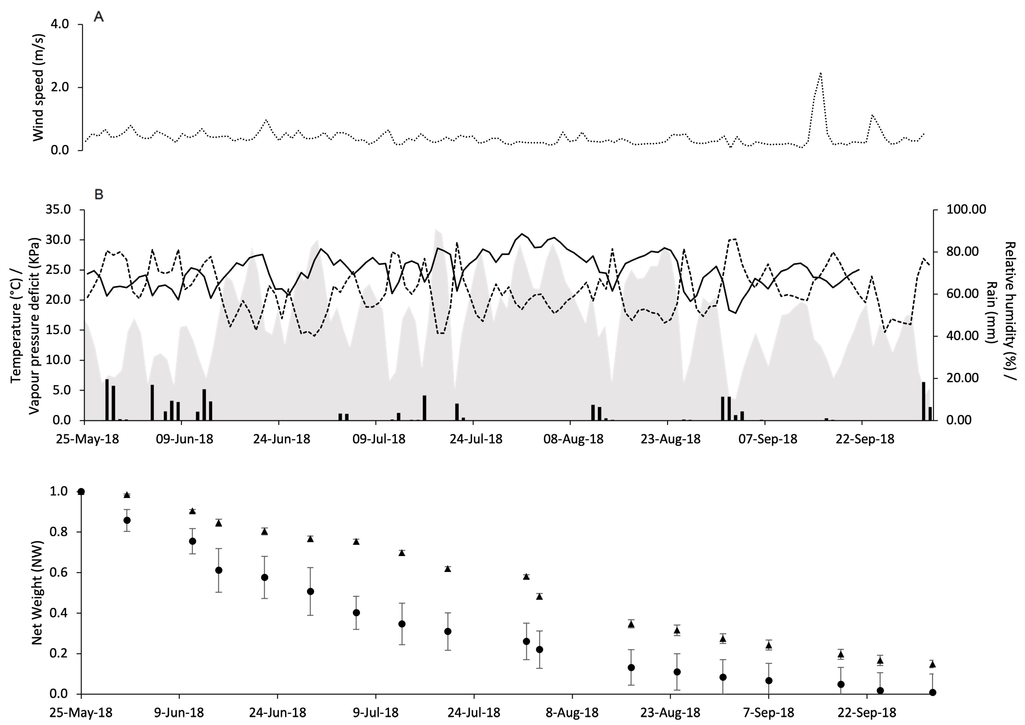
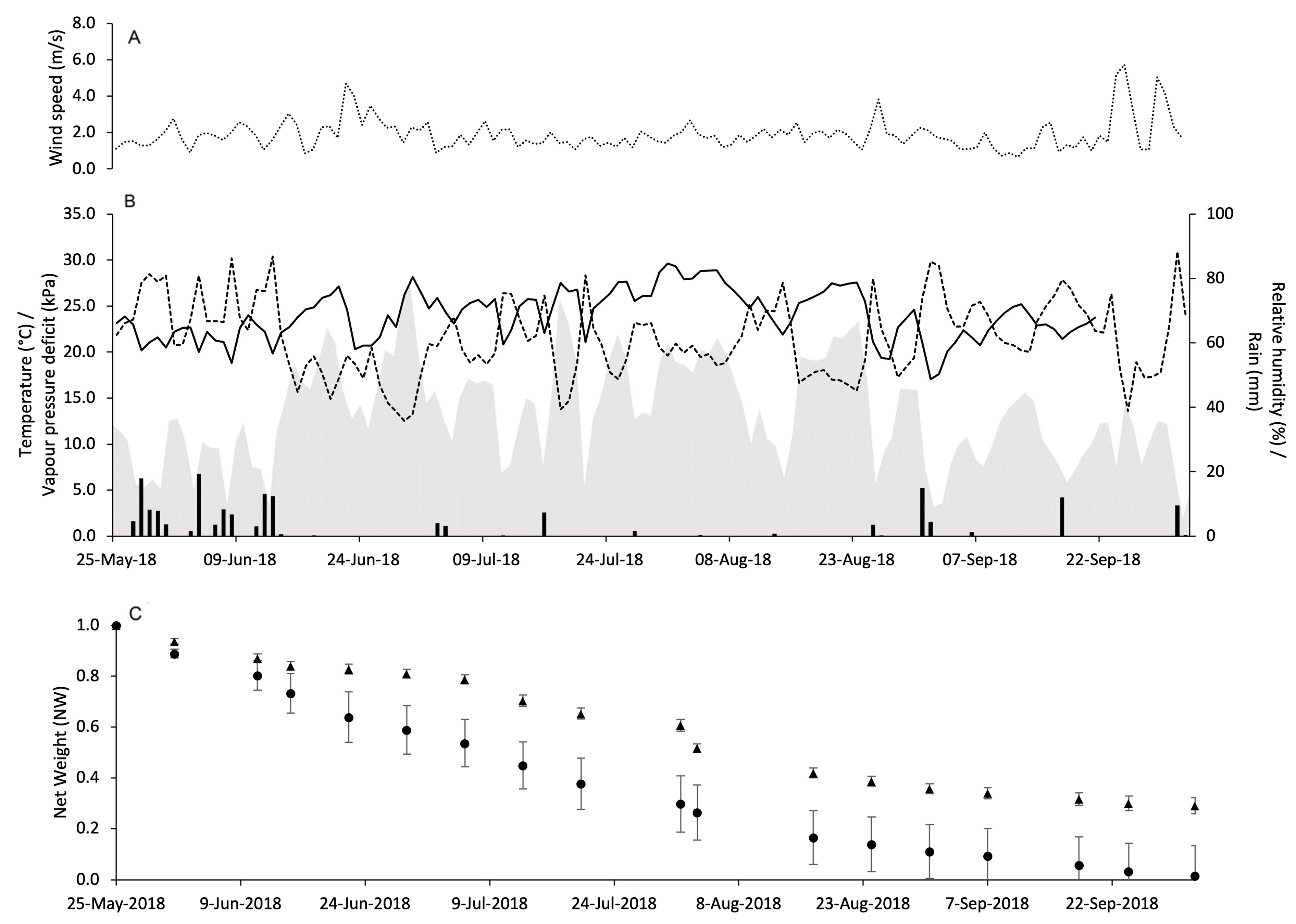
2.3. Pheromone Release Under Vineyard Conditions

The experiment was conducted in 2017 and 2018 in an experimental vineyard at the Università Cattolica del Sacro Cuore campus (Piacenza, PC, 45°2′15.4536″ N, 9°43′46.326″ E; 80 m above sea level [a.s.l.]) and in 2018 in two commercial vineyards of the Colli piacentini denomination, at Castell’Arquato (CA, 44°51′26.0352″ N, 9°51′17.9748″ E; 400 m above sea level [a.s.l.]), and Vicobarone (VB, 44°59′31.542″ N, 9°21′28.0656″ E; 375 m above sea level [a.s.l.]). The vines at PC were two years old in 2017; they were trained using a Guyot system with within- and between-row spacings of 0.9 and 1 m, respectively. At CA, the vineyard was 11 years old in 2018, and plants were trained using a Guyot system. The within- and between-row spacings were 1.0 and 2.3 m, respectively. At VB, plants were two years old in 2018 and trained using a Guyot system; the within- and between-row spacings were 1.2 and 3 m, respectively.
In each vineyard, hourly data of temperature (T, in °C), relative humidity (RH, in %), rainfall (R, in mm), and wind speed (WS, in m/s) were recorded using an automated weather station (iMeteos; Pessl Instruments GmbH, Weiz, Austria) located < 1 km from the experimental plots. The growth stages of vines were assessed weekly in the vineyards according to the scale of Lorenz et al. [32].
At the PC vineyard, five dispensers per type (Isonet and Rak) were hung in the vineyard on 23 May 2017 and on 25 May 2018. At VB and CA vineyards, 90 dispensers per type were hung on 25 May 2018. The dispensers were collected at 7-day intervals, transported to the laboratory in a fridge, and weighed as described before. At the PC vineyard, considering the proximity of the vineyard to the laboratory, the dispensers were relocated soon after weighing and collected again 1 week after. At the VB and CA vineyards, 5 dispensers per type were collected at each sampling date, and after the weight measure, they were discarded as plant protection products. The sampling period was between 125 and 151 days based on the year. The tare of each dispenser was determined at the end of the sampling period, as previously described.
The NW of dispensers at any sampling time in any vineyard and year was calculated and rescaled to estimate the PR (on a 0 to 1 scale), as a relative reduction in dispenser NW, as described before. The rescaled data were then fit through a linear regression with the following general equation:
PR = α + β1X1 + β2X2 + … + βnXn + ε
where α and β1 to βn are equation parameters, ε is the error, and X1 to Xn are the following independent variables: (i) day of the year (DOY), (ii) accumulated values of PRR (ΣPRR) from the experiment under controlled conditions, (iii) degree days accumulated when temperature > 0 °C (ΣDD, in °C), (iv) accumulated daily precipitation (ΣDP, in mm), and (v) accumulated daily vapor pressure deficit (ΣVPD, in kPa) with the VPD being calculated as follows [33]: VPD = 0.61121 exp((18.678 − T/234.5)(T/(257.14 + T)))(1 − RH/100). Hourly meteorological data were transformed to obtain the daily averages of temperature and relative humidity. In (ii) and (iii), we were interested in evaluating the dynamics of PR over a temperature-dependent physiological time [34]. In (iv) and (v), we searched for a possible effect of rain or evaporative atmospheric potential on PR [35].
In the first set of equations, the independent variables were first used individually in a linear (i.e., with the term Xn only) and polynomial (i.e., with Xn and Xn2). In the second set, the independent variables and their squared values were used altogether in a stepwise regression, which is a step-by-step method for adding and removing terms from a multilinear model based on their statistical significance in a regression. At each step, the independent variable not in the equation with the smallest probability of F is entered if that probability is <0.05; variables already in the regression equation are removed if their probability of F becomes >0.10. The method terminates when no more variables are eligible for inclusion or removal.
In a third set of equations, four dichotomous variables (with values 0 or 1) accounting for single vineyards (PC17, PC18, CA18, and VC18) were also included in a stepwise regression. Such inclusion was made to verify whether there are vineyard-specific conditions that are not related to the time (DOY) and weather-related variables (ΣPRR, ΣDD, ΣDP, and ΣVPD).
Equation parameters were estimated using the function nls of the “stats” package of R software (R, 2020). The parameterized equations were evaluated based on the standard error of estimates (SEest), Radj2, AIC, RMSE, CRM, and CCC. Only relevant equations were reported in the following sections.

3. Results

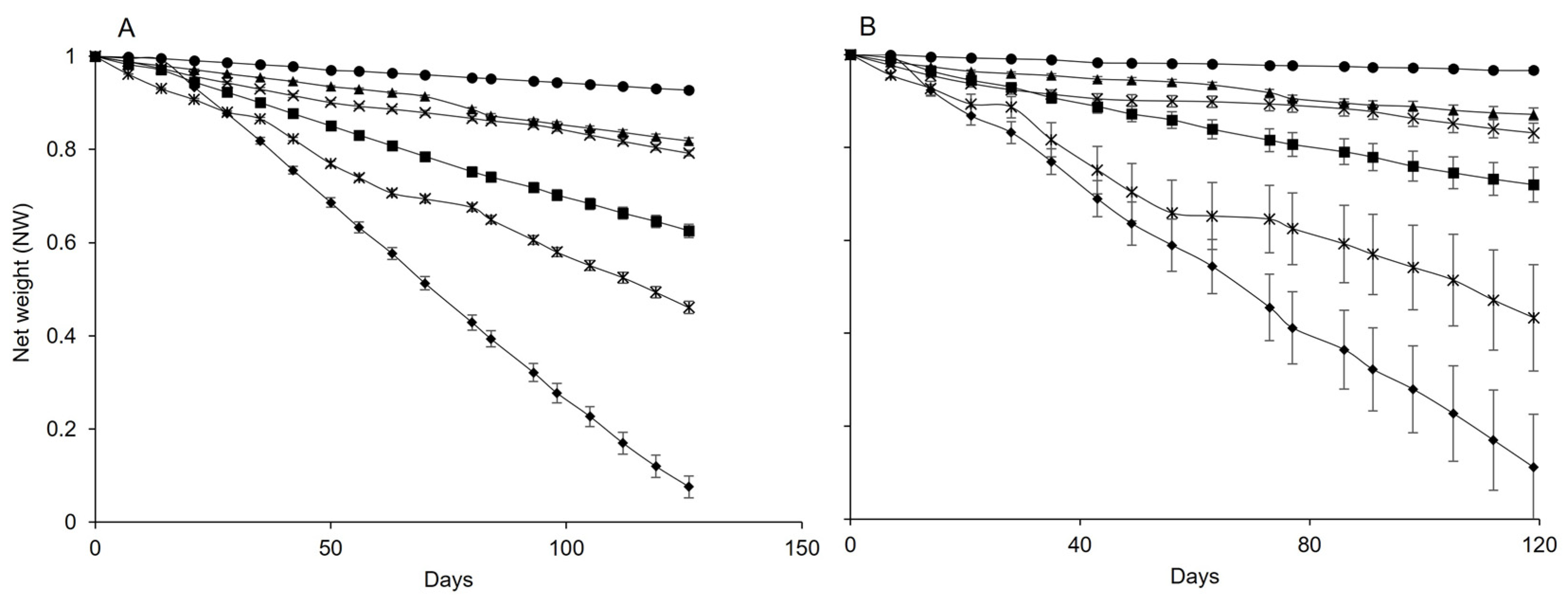
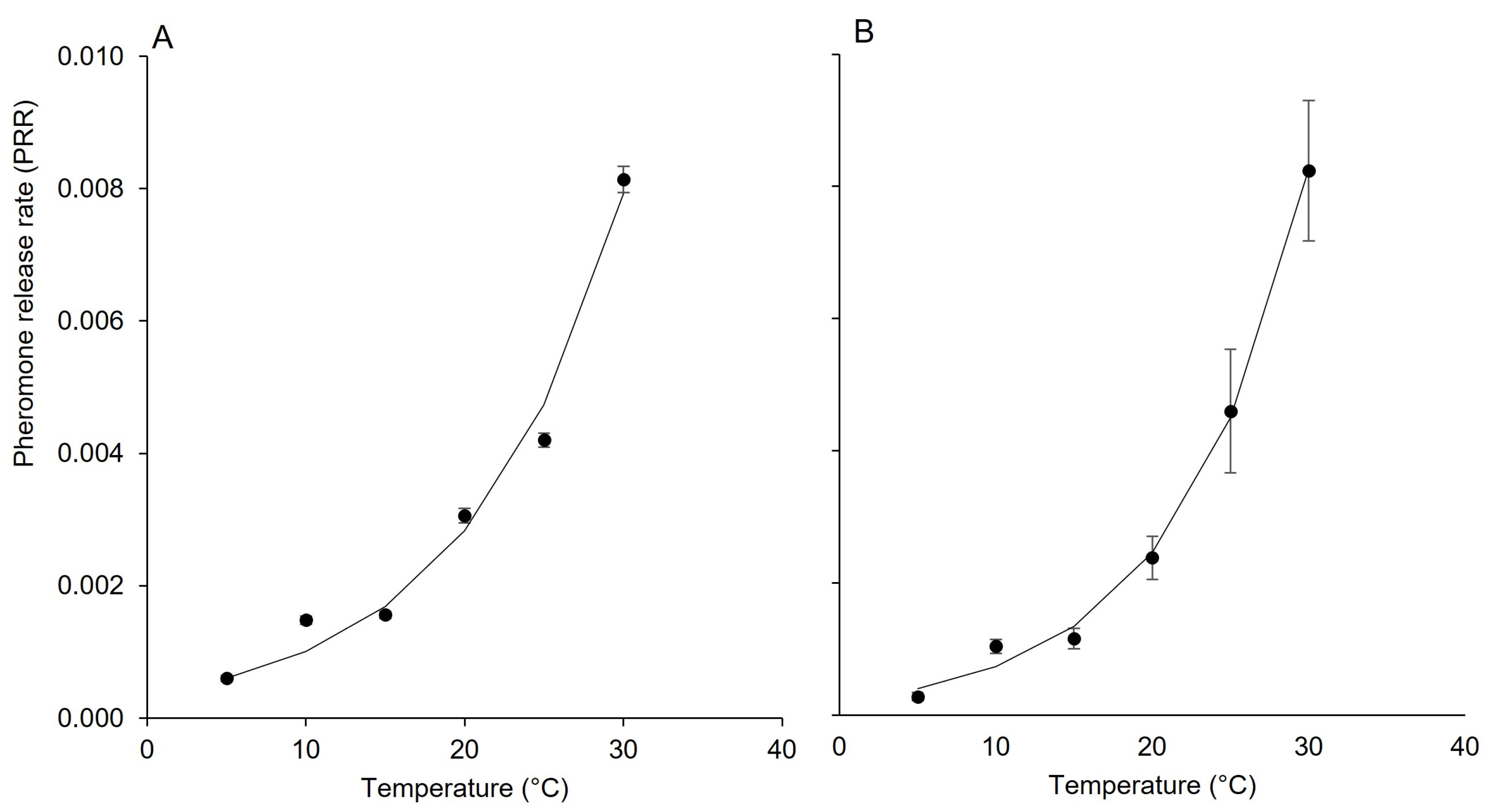
3.1. Effect of Temperature on Pheromone Release

For both dispensers, the highest weight loss was obtained at 30 °C with a difference between the average initial weight (Wi) and the average final weight (Wf) of 0.480 g and 0.337 g for Isonet and Rak, respectively (Table 1). The lowest weight loss was observed at 5 °C with values of 0.038 g and 0.014 g for Isonet and Rak, respectively.
The net weights of both dispensers decreased over the sampling date for about 120 days; no further weight changes were observed afterward. However, the slope at which dispensers lost weight differed at the selected temperatures (Figure 1A,B). Therefore, the slopes of the weight reductions differed (Table 1).
The dynamic of PRR (i.e., the pheromone release rate over time) for each dispenser was finally calculated using the following exponential equation:
P R R = α e β T
where α and β are equation parameters representing the lower limit of PRR and the intrinsic rate of increase in response to temperature (T, in °C) (Figure 2A,B).
Equation (3) provided a good data fit (Table 2).

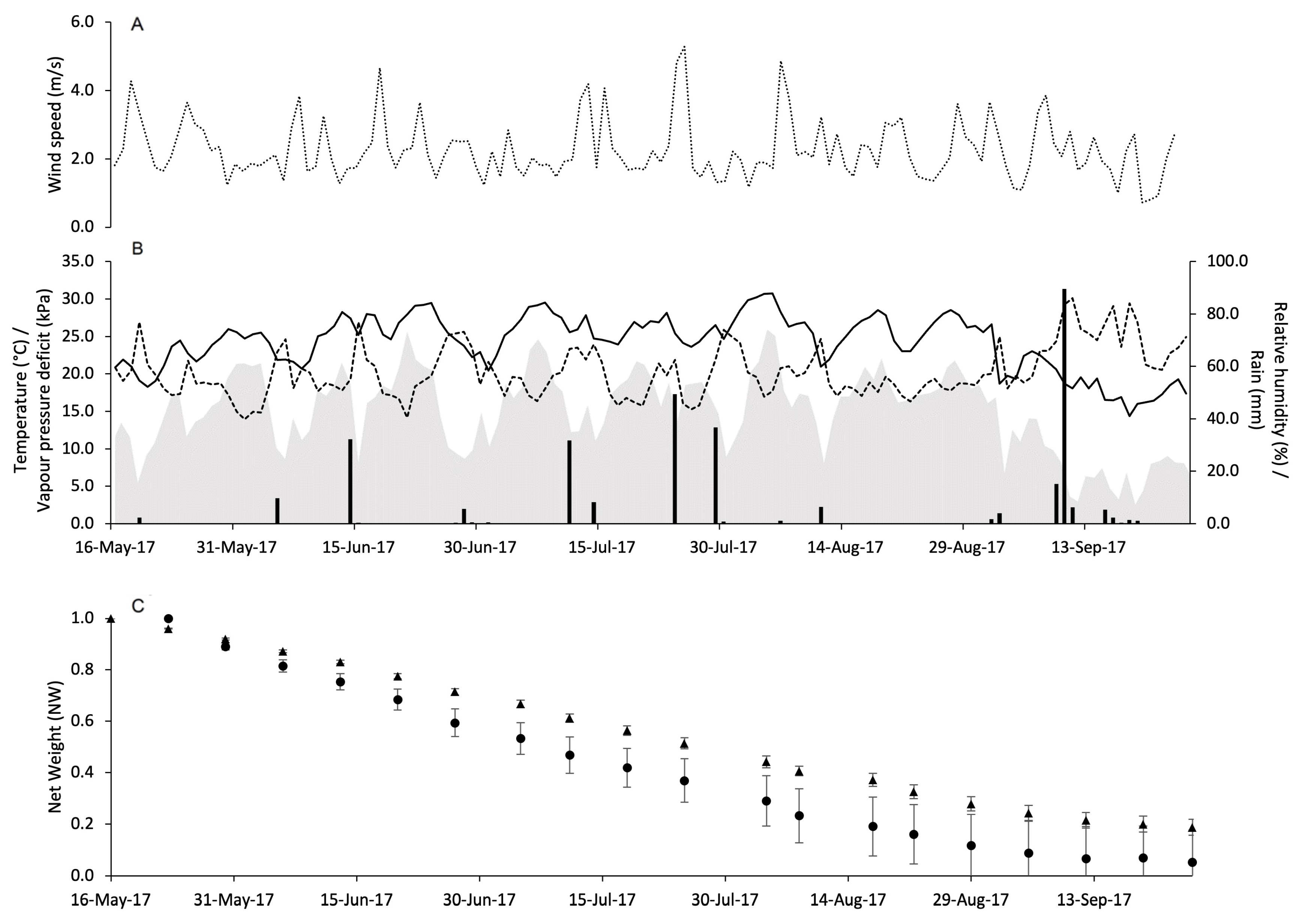
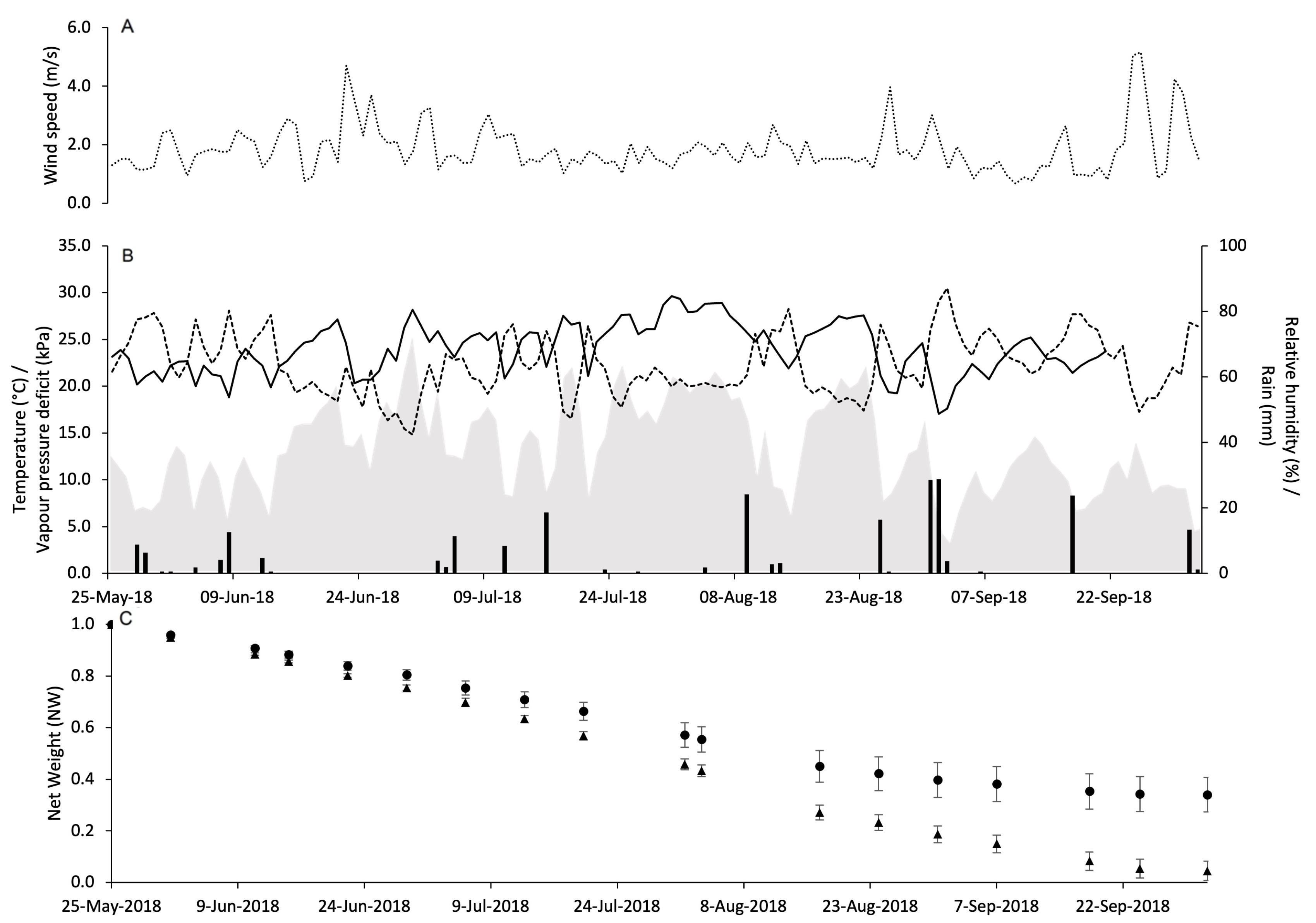
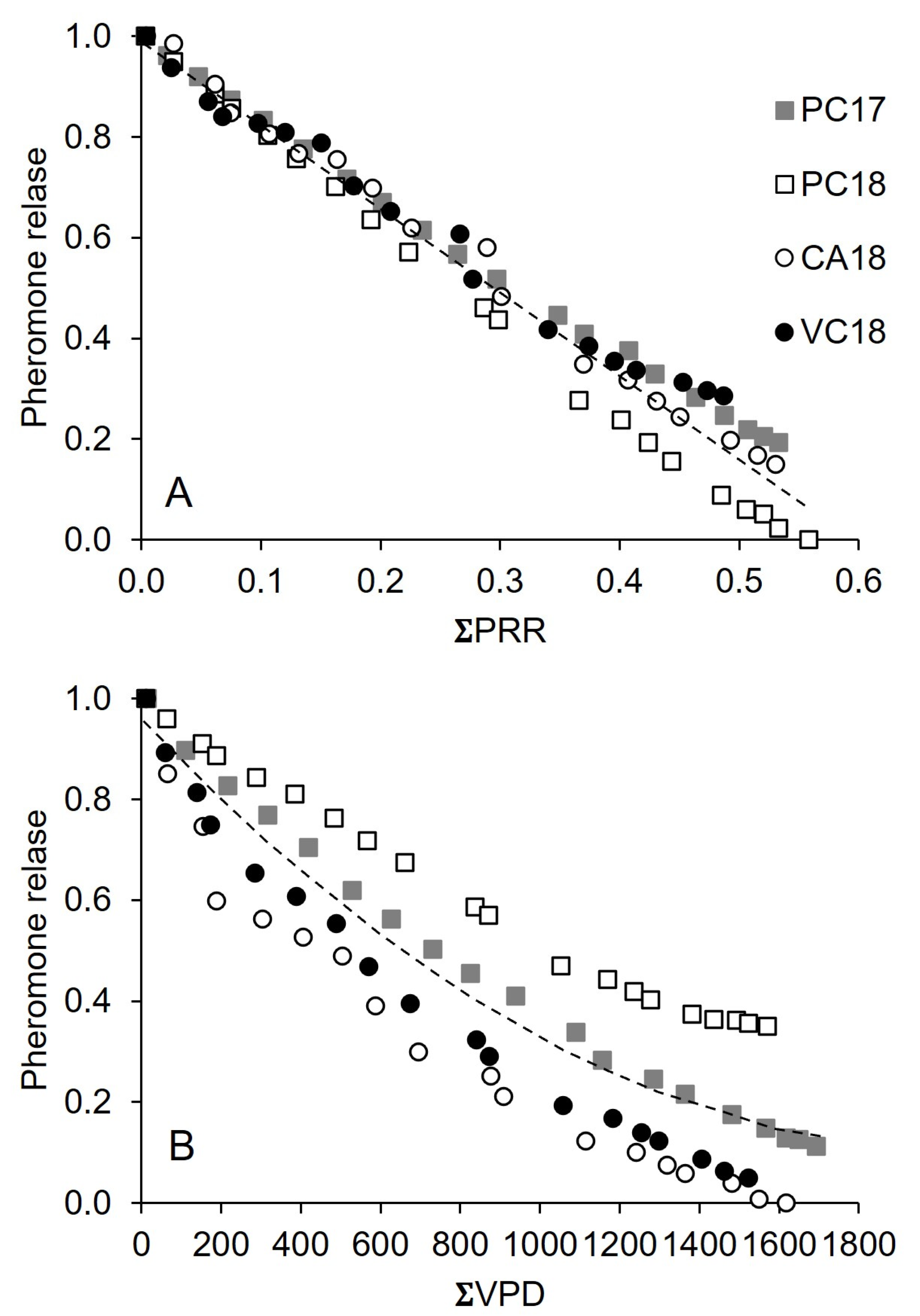
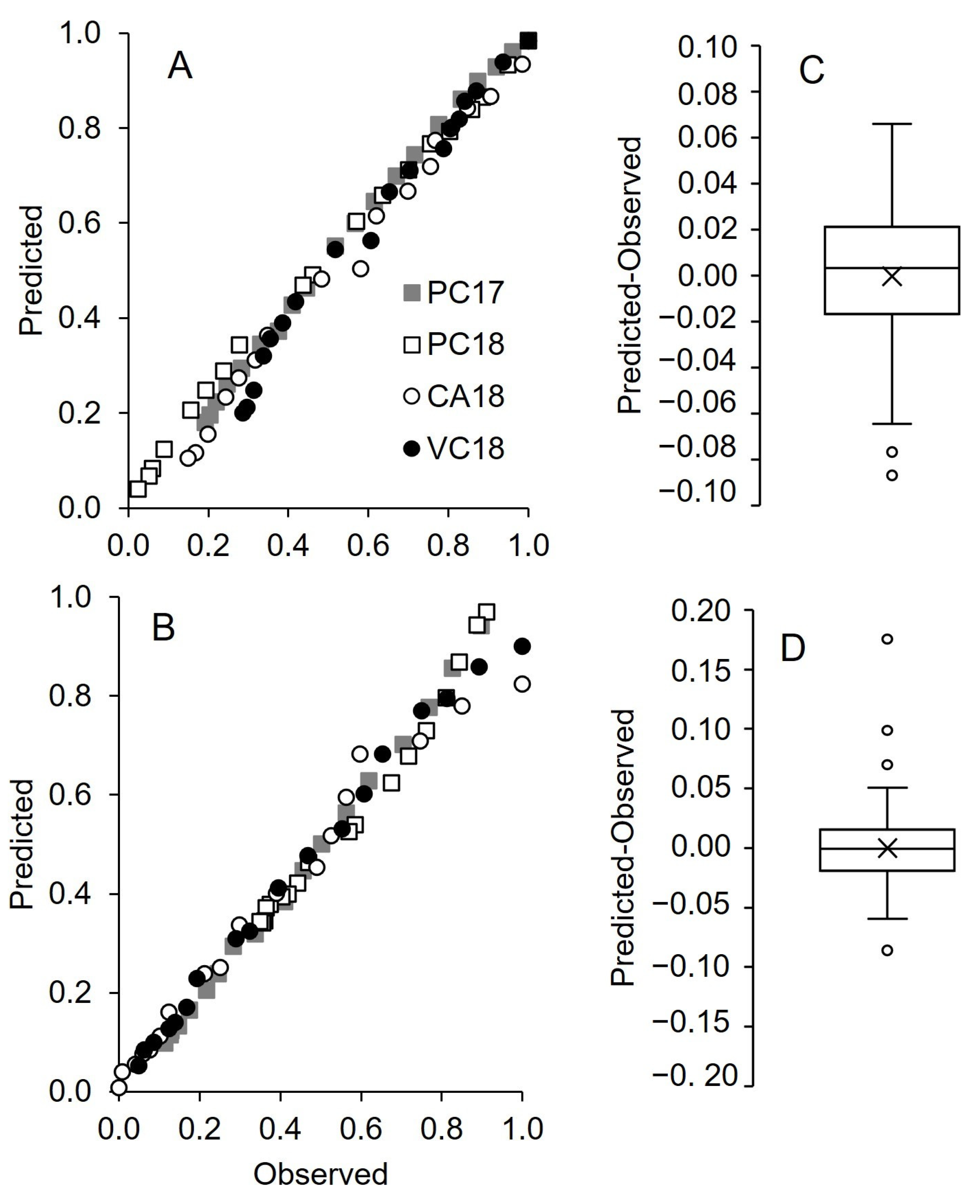
3.2. Pheromone Release Under Vineyard Conditions

Weather conditions during the use of pheromone dispensers in vineyards were quite variable. At PC in 2017, WS remained almost constant with some peaks above 4 m/s (Figure 3A). The total amount of rain during the experimental period was 314 mm with peaks > 30 mm on June 14 (32.2 mm), July 11 (31.8 mm), July 24 (49.4 mm), July 29 (36.8 mm), and September 10 (89.6 mm). The daily temperature ranged from 14.4 to 30.8 °C with an overall average of 24.2 °C. The average VPD was 1.3 kPa and ranged from 0.3 to 2.3 kPa (Figure 3B).
At PC in 2018, WS was similar to that observed in 2017 with fewer peaks above 4 m/s (Figure 4A). However, the weather was a little bit dryer and cooler than 2017. Indeed, there was 274.7 mm of rain during the experimental period, and the daily temperature ranged from 12.2 to 30.4 °C with an average of 23.1 °C. The VPD ranged from 0.2 to 2.2 kPa with an overall average of 1 kPa (Figure 4B).
At CA in 2018, WS was constantly close to 0 with a maximum of 2.5 m/s on 16th September (Figure 5A). A total of 208.7 mm of rain fell during the experimental period. The daily temperature ranged from 13.2 to 31 °C, and the average was 24.4 °C. The average daily VPD was 1.2 kPa, ranging from 0.3 to 2.3 kPa (Figure 5B).
At VB in 2018, three days above 5 m/s were registered: September 24 (5.1 m/s), September 25 (5.7 m/s) and September 29 (5.0 m/s) (Figure 6A). In total, 175.4 mm of rain fell during the experimental period. The daily temperature ranged from 12.9 °C to 29.6 °C, and the average was 23.5 °C. The average daily VPD was 1.2 kPa, ranging from 0.2 to 2.4 kPa (Figure 6B).
The dynamics over time of PR by Isonet and Rak dispensers in the four vineyards are shown in panels C of Figure 3, Figure 4, Figure 5 and Figure 6. In general, NW loss has a linear trend with no peaks of decline.
For Isonet, the linear regression with ΣPRR as an independent variable provided the best fit of PR (Table 3); the use of ΣDD also provided a good fit, and both were more accurate than DOY (for instance, AIC decreased by 25 and 21, respectively), indicating that temperature had a relevant role in PR.
Regression with ΣDP and ΣVPD provided a worse fit than temperature-related variables (Table 3), indicating that rain and VPD had poor explanatory power when used singly. The use of square terms through polynomial regression for individual independent variables never showed a significant contribution, meaning that the decline in pheromone release over the selected independent variables was linear (Figure 7A).
Two variables, ΣPRR and ΣVPD, were linearly combined when all independent variables were used in stepwise regression, providing a relevant increase in goodness-of-fit (Table 3) and precision of estimates. The SEest was 0.046 for the regression with ΣPRR only and 0.032 for the regression with ΣPRR and ΣVPD (Table 3). Therefore, the evaporative potential of the atmosphere (namely, the difference between the amount of moisture in the air and how much moisture the air can hold when saturated) played a relevant role in combination with temperature. Dichotomic variables related to single vineyards were never significantly included in the regression equation, indicating no considerable differences among vineyards.
For Rak, the best fit among the regressions with single independent variables was obtained with ΣVPD (Table 4) even though the differences among variables were less evident than for Isonet (cfr. Table 3).
Unlike Isonet, the quadratic term in polynomial regressions was always notable, meaning that the reduction in pheromone release was not linear (Figure 7B, referring to VPD). As for Isonet, the stepwise regression selected two linearly combined variables, ΣPRR2 and ΣVPD, which provided some increase in the goodness-of-fit, which remained lower than for Isonet (Table 4). However, the fit to real data significantly increased (e.g., the AIC went from −327 to −480), and the estimates were more accurate (e.g., the SEest went from 0.111 to 0.039) when the dichotomic variable for vineyards was included in the analysis.
The comparison between predicted values based on the above regression equations and observed values of pheromone release is shown in Figure 8. The differences between the distribution of predicted and observed values are shown in Figure 8B,D, for Isonet and Rak, respectively. For both dispensers, the interquartile range is between −0.05 and 0.05, with the average close to 0, stating the good prediction of the chosen equations.

4. Discussion

MD has traditionally been used as an environmentally friendly method for controlling L. botrana and E. ambiguella using different dispensers for specific pheromones. These include sprayable formulations [36], female-equivalent dispensers [37], automatic aerosol devices [38], and hand-applied passive dispensers [39,40]. Among these dispensers, we selected the passive dispensers Isonet and Rak because they have been widely used to control EGVM and EGBM [19,41,42,43]. These dispensers are considerably different in shape, and it is known that dispenser shape and material influence the pheromone release [44].
Isonet consists of two parallel, thin ropes of polymeric material, one filled with pheromone welded at the ends and open in the center to allow application on the plant. Isonet technology allows pheromone release to be constant and regular during the season. The dispenser wall, which is characterized by many small pores, remains impregnated with the active substance by capillarity throughout the season even when its content is decreasing; this ensures a constant flow of pheromones from the diffuser to the environment [25]. The Rak dispenser is made of porous plastic with two ampoules containing the active substance. In this type of dispenser, the liquid pheromone permeates outside by exploiting the characteristics of the plastic material in which it is contained. Once on the external wall, the pheromone volatilizes and spreads into the environment [44,45].
The different shapes of the two dispensers may have influenced the PR patterns observed [46]. Isonet has an approximate surface area of A = 17.2 cm2 and a volume of V = 1.69 cm3, which results in a surface area-to-volume ratio of 10.15 (1/cm); Rak has A = 20.1 cm2, V = 6.97 cm3, with a surface area-to-volume ratio of 2.88 (1/cm) [47]. This ratio was 3.5 times higher in Isonet than in Rak, affecting pheromone release dynamics. The porosity (e.g., type, number per surface unit, and size of pores) of the dispenser materials may also influence the release, but details on these characteristics are not available. It may also be considered that Rak contains a substance (N-dodecenyl acetate) that delays pheromone release (which is absent in Isonet), which could, to some extent, influence the pheromone release dynamic over time.
For both dispensers, temperature and VPD explained the PR in vineyards characterized by diverse weather conditions better than time; this is consistent with the mechanism of pheromone evaporation from the dispenser surface and its consequent rewetting by capillarity. Indeed, VPD essentially represents how easily water evaporates; a low VPD means that water evaporates slowly, while increasing VPD indicates increased evaporation. Low temperatures yielded a low VPD at a fixed RH, while high temperatures resulted in a high VPD [48]. Therefore, pheromone evaporation from the dispenser surface may be higher at high VPD than at low VPD. Additionally, as the temperature of the pheromone increases, its surface tension diminishes, and this facilitates attractive forces between pheromone molecules and dispenser walls to pull the internal liquid into capillary pores and wet pheromone molecules out [49]. In our preliminary experiment, the effect of temperature on PRR was not linear, and any temperature increase at high temperatures accelerated the release rate more than proportionally. Zhu et al. [24] obtained similar results with dispensers different from the ones we used.
Weather conditions, particularly temperature, have been previously observed to potentially influence pheromone release [50,51,52,53]. For instance, Moschos et al. [54] observed that pheromone release by the Rak 2 Plus dispenser in a 3-year period (1996–1998) was high in July and minimal in April and September–October due to hot temperatures in the summer months. Arn et al. [50] found that the pheromone release rate by the Rak 1 + 2 ampoule increased by a factor of 10 from 15 to 35 °C and observed that this temperature-dependent release does not match the male activity of moths, which was high between dusk and the end of the scotophase when temperatures were low [2,50]. Van der Kraan and Ebbers [55] noticed a 2–2.5-fold increase in the pheromone emission by polythene tubes with a rise in temperature between 15 °C and 25 °C. Our results are in agreement with previous studies. However, the exponential function we used for studying the temperature-dependent PRR under field conditions better fits real data than degree days, confirming the non-linear effect of temperature.
The effect of wind and RH has been considered of no or minor importance in previous studies [23,56,57] even though there was evidence of the effect of certain wind speeds on the increase in pheromone release [23,46,55,58] and of high humidity on the release reduction [24,59,60] under environment-controlled conditions. Indeed, increased wind speeds may facilitate the volatilization of pheromones from dispenser surfaces, thus increasing the mobility of the inner molecules [23,24,44,46,61]. Additionally, high environmental humidity may have the opposite effect. The considerable impact of VPD on PR in our study under vineyard conditions would indirectly support the role of wind and humidity, as RH is directly related to VPD, and wind is related to RH levels [62]. In another field study, Gavara et al. [63] found that daily pheromone release rates by an Isonet dispenser were predicted (with R2 = 0.378) by a multiple regression that included minimum and maximum daily temperatures and average WS. Precipitation had no notable effect in our study nor the study of Gavara et al. [63].
In contrast to Isonet, Rak showed a non-linear release trend of the pheromone emission in all tested field conditions; further, the stepwise regression pointed out the importance of the dichotomous variable of the vineyard to increase goodness of fit. This effect may be due to the pheromone-absorbing capacity of the canopy, as shown in several publications [64]. The waxy surface of the leaves seems to be the site responsible for the uptake and release of pheromones by plants, considering also that the ground cover might affect in minimal part the absorption of the pheromone [21]. Gavara et al. [25] suggested that the plant canopy is unnecessary to achieve MD with passive dispensers. Still, it may keep the pheromone in the field area, leading to a more uniform distribution and an increase in the number of pheromone sources along the crop, consequently improving the competitive mechanisms of disruption. The MD competitive mechanism, i.e., false trails formation, is achieved when artificial sources emitting pheromones overcome plumes produced by adult females. On the other hand, a non-competitive mechanism, i.e., the desensitization of males, typically takes place when moths are exposed to huge concentrations of pheromones, which is hardly obtained in vineyards treated with MD dispensers [65,66]. Studies have shown that the competitive mechanism is more exerted in MD control for EGVM. On the contrary, EGBM females produce a very attractive blend of pheromones, critically influencing the competitive mechanism in MD [19].
Our results were obtained by estimating PR by measuring the weight loss of dispensers over time, as in previous studies (e.g., [22,67,68]). It could then be questioned if this method reflects the emission of pheromones into the vineyard air, in case the dispenser weight loss was caused by the loss of other volatile components eventually present in the dispenser, by the decomposition of some dispenser materials, or because precipitation and moisture influence the absorption and desorption of water by dispensers [22]. An alternative method is extracting residual pheromone from the dispenser using gas chromatography [11]. In a comparative study under field conditions, however, Il’ichev et al. [36] found that the weight loss method and gas chromatography provided comparable results. The weight loss method is non-destructive, does not require expensive equipment, and is cheaper. Additionally, it can be easily used in routine evaluations within MD programs, increasing the exploitation of our results. Our results indicate that weather conditions influencing pheromone release (namely, air temperature and VPD) may be common for different dispenser types [23]. However, our equations were dispenser-dependent, so equations relating these influencing variables to the pheromone release pattern must be defined for each dispenser type.

5. Conclusions

The equations developed in this work can potentially be used in the management of pheromone dispensers for MD. Effective MD requires dispensers application before the first flight of the moths [69] and the coverage of all flights until the harvest, which are especially critical with late season varieties [63]. These equations, eventually linked to mathematical models predicting the phenology of EGVM [70] and EGBM [71] populations, may support the farmers in advance about the right moment for the dispenser’s application and the pheromone release available to disrupt during flights. Indeed, these equations can provide information on the PR during the season, as influenced by weather conditions. Since the dispensers need to ensure the release of a sufficient pheromone dose to disrupt the mating of the target pests across different pest generations, these equations could serve as an input for an atmospheric pheromone concentration model to predict concentrations based on meteorological conditions [72]. However, the equations should be further validated against independent data collected under diverse environmental conditions before use. These validation efforts should also consider the efficacy of MD through pheromone traps for monitoring the adult male population and sampling eggs, larvae, and damaged barriers.

Author Contributions

Conceptualization, V.R., L.B. and G.F.; Methodology, V.R., L.B. and G.F.; Formal Analysis, M.C., L.B. and G.F.; Data curation, M.C., L.B. and G.F.; Writing—Original Draft Preparation, M.C. and G.F.; Writing—Review and Editing, M.C., V.R. and G.F.; Visualization, M.C. and G.F. All authors have read and agreed to the published version of the manuscript.

Funding

This research received no external funding.

Data Availability Statement

The raw data supporting the conclusions of this article will be made available by the authors without undue reservation.

Conflicts of Interest

Author Luca Bricchi conducted the experiments during his master thesis and was not employed by the company Consorzio agrario Terrepadane scrl at that time. The remaining authors declare that the research was conducted in the absence of any commercial or financial relationships that could be construed as a potential conflict of interest.

References

  1. Louis, F.; Schirra, K.-J. Mating disruption of Lobesia botrana (Lepidoptera: Tortricidae) in vineyards with very high population densities. IOBC WPRS Bull. 2001, 24, 75–80. [Google Scholar]
  2. Lucchi, A.; Sambado, P.; Juan Royo, A.B.; Bagnoli, B.; Benelli, G. Lobesia botrana males mainly fly at dusk: Video camera-assisted pheromone traps and implications for mating disruption. J. Pest Sci. 2018, 91, 1327–1334. [Google Scholar] [CrossRef]
  3. Thiéry, D. Les Vers de la Grappe, les Connaître pour s’en Protéger; Vigne et Vins International: Bordeaux, France, 2005; p. 60. [Google Scholar]
  4. Varner, M.; Lucin, R.; Mattedi, L.; Forno, F. Experience with mating disruption technique to control grape berry moth, Lobesia botrana. IOBC WPRS Bull. 2001, 24, 81–88. [Google Scholar]
  5. Fermaund, M.; Le Menn, R. Association of Botrytis cinerea with grape berry moth larvae. Phytopathology 1989, 79, 651–656. [Google Scholar] [CrossRef]
  6. Ioriatti, C.; Anfora, G.; Tasin, M.; De Cristofaro, A.; Witzgall, P.; Lucchi, A. Chemical ecology and management of Lobesia botrana (Lepidoptera: Tortricidae). J. Econ. Entom. 2011, 104, 1125–1137. [Google Scholar] [CrossRef] [PubMed]
  7. Vartholomaiou, A.N.; Navrozidis, E.I.; Payne, C.C.; Salpiggidis, G.A. Agronomic Techniques to Control Lobesia botrana. Phytoparasitica 2008, 36, 264–271. [Google Scholar] [CrossRef]
  8. Ioriatti, C.; Lucchi, A. Semiochemical Strategies for Tortricid Moth Control in Apple Orchards and Vineyards in Italy. J. Chem. Ecol. 2016, 42, 571–583. [Google Scholar] [CrossRef]
  9. Duso, C.; Pozzebon, A.; Lorenzon, M.; Fornasiero, D.; Tirello, P.; Simoni, S.; Bagnoli, B. The Impact of Microbial and Botanical Inseticides on Grape Berry Moths and Their Effects on Secondary Pests and Beneficials. Agronomy 2022, 12, 217. [Google Scholar] [CrossRef]
  10. Shailaja, D.; Ahmed, S.M.; Yaseen, M. Comparative study of release kinetics of pheromone from polymer dispensers. J. Appl. Polym. Sci. 1997, 64, 1373–1380. [Google Scholar] [CrossRef]
  11. Gavara, A.; Vacas, S.; Navarro, I.; Primo, J.; Navarro-Llopis, V. Airborne pheromone quantification in treated vineyards with different mating disruption dispensers against lobesia botrana. Insects 2020, 11, 289. [Google Scholar] [CrossRef]
  12. Harari, A.R.; Zahavi, T.; Steinitz, H. Female detection of the synthetic sex pheromone contributes to the efficacy of mating disruption of the European grapevine moth, Lobesia botrana. Pest Manag. Sci. 2015, 71, 316–322. [Google Scholar] [CrossRef] [PubMed]
  13. Cardé, R.T. Principles of mating disruption. In Behavior-Modifying Chemicals for Pest Management: Applications of Pheromones and Other Attractants; Marcel Dekker: New York, NY, USA, 1990; pp. 47–71. [Google Scholar]
  14. Bartell, R.J. Mechanisms of communication disruption by pheromone in the control of Lepidoptera: A review. Physio. Entom. 1982, 7, 353–364. [Google Scholar]
  15. Justum, A.R.; Gordon, R.F.S. Pheromones: Importance to insects and role in pest management. In Insect Pheromones in Plant Protection; John Wiley & Sons: New York, NY, USA, 1989; pp. 1–13. [Google Scholar]
  16. Ridgway, R.L.; Inscoe, M.N.; Dickerson, W.A. Role of the boll weevil pheromone in pest management. In Behavior-Modifying Chemicals for Insect Management; Ridgway, R.L., Silverstein, R.M., Inscoe, M., Eds.; Marcel Dekker: New York, NY, USA, 1990; pp. 437–471. [Google Scholar]
  17. Teja, R.R. Novel Green Technologies for Pest Control. Just. Agric. 2022, 2, 1–5. [Google Scholar]
  18. Pasquier, D.; Charmillot, P. Survey of pheromone emission from different kinds of dispensers used for mating disruption in orchards and vineyards. IOBC WPRS Bull. 2005, 9, 335–339. [Google Scholar]
  19. Ioriatti, C.; Bagnoli, B.; Lucchi, A.; Veronelli, V. Vine moths control by mating disruption in Italy: Results and future prospects. Redia 2005, 87, 117–128. [Google Scholar]
  20. EPPO. PP 1/264 (2) Principles of efficacy evaluation for mating disruption pheromones. EPPO Bull. 2019, 49, 426–430. [Google Scholar] [CrossRef]
  21. Sauer, A.E.; Karg2, G. Variables affecting pheromone concentration in vineyards treated for mating disruption of grape vine moth Lobesia botrana. J. Chem. Ecol. 1998, 24, 289–302. [Google Scholar] [CrossRef]
  22. Koch, U.T.; Quasthoff, M.; Klemm, M.; Becker, J. Methods for reliable measurement of pheromone dispenser performance. IOBC WPRS Bull. 2002, 25, 95–99. [Google Scholar]
  23. Hofmeyr, J.H.; Burger, B.V. Controlled-release pheromone dispenser for use in traps to monitor flight activity of false codling moth. J. Chem. Ecol. 1995, 21, 355–363. [Google Scholar] [CrossRef]
  24. Zhu, H.; Thistle, H.W.; Ranger, C.M.; Zhou, H.; Strom, B.L. Measurement of semiochemical release rates with a dedicated environmental control system. Biosyst. Eng. 2015, 129, 277–287. [Google Scholar] [CrossRef]
  25. Vidal, A.G. Cuantificación de Feromonas en Aire y su Aplicación en Métodos de Control de Plagas. Ph.D. Thesis, Universitat Politècnica de València, Valencia, Spain, 2021. [Google Scholar]
  26. Akaike, H. Likelihood of a model and information criteria. J. Econ. 1981, 16, 3–14. [Google Scholar] [CrossRef]
  27. Lin, L.I. A concordance correlation coefficient to evaluate reproducibility. Biometrcs 1989, 45, 255–268. [Google Scholar] [CrossRef]
  28. Nash, J.E.; Sutcliffe, J.V. River flow forecasting through conceptual models part I–a discussion of principles. J. Hydrol. 1970, 10, 282–290. [Google Scholar] [CrossRef]
  29. Wickham, H.; Averick, M.; Bryan, J.; Chang, W.; McGowan, L.; François, R.; Grolemund, G.; Hayes, A.; Henry, L.; Hester, J.; et al. Welcome to the Tidyverse. J. Open Source Softw. 2019, 4, 1686. [Google Scholar] [CrossRef]
  30. Signorell, A. DescTools: Tools for Descriptive Statistics, R Package Version 0.99.53. 2024.
  31. Madden, L.V.; Gareth, H.; van den, B.F. The Study of Plant Disease Epidemics; APS Publications: Rockville, MD, USA, 2017; p. 421. [Google Scholar]
  32. Lorenz, D.H.; Eichhorn, K.W.; Bleiholder, H.; Klose, R.; Meier, U.; Weber, E. Growth Stages of the Grapevine: Phenological growth stages of the grapevine (Vitis vinifera L. ssp. vinifera)—Codes and descriptions according to the extended BBCH scale. Aust. J. Grape. Wine. Res. 1995, 1, 100–103. [Google Scholar] [CrossRef]
  33. Buck, A.L. New equations for computing vapor pressure and enhancement factor. J. Appl. Meteorol. Climatol. 1981, 20, 1527–1532. [Google Scholar] [CrossRef]
  34. Tobin, P.C.; Zhang, A.; Onufrieva, K.; Leonard, D.S. Field evaluation of effect of temperature on release of disparlure from a pheromone-baited trapping system used to monitor gypsy moth (Lepidoptera: Lymantriidae). J. Econ. Entomol. 2011, 104, 1265–1271. [Google Scholar] [CrossRef]
  35. Klassen, D.; Lennox, M.D.; Dumont, M.J.; Chouinard, G.; Tavares, J.R. Dispensers for pheromonal pest control. J. Environ. Manag. 2023, 325, 116590. [Google Scholar] [CrossRef]
  36. Il’ichev, A.L.; Williams, D.G.; Gut, L.J. Dual pheromone dispenser for combined control of codling moth Cydia pomonella L. and oriental fruit moth Grapholita molesta (Busck) (Lep., Tortricidae) in pears. J. Appl. Entomol. 2007, 131, 368–376. [Google Scholar] [CrossRef]
  37. Stelinski, L.L.; McGhee, P.; Grieshop, M.; Brunner, J.; Gut, L.J. Efficacy and mode of action of female-equivalent dispensers of pheromone for mating disruption of codling moth. Agric. For. Entomol. 2008, 10, 389–397. [Google Scholar] [CrossRef]
  38. Benelli, G.; Lucchi, A.; Thomson, D.; Ioriatti, C. Sex pheromone aerosol devices for mating disruption: Challenges for a brighter future. Insects 2019, 10, 308. [Google Scholar] [CrossRef] [PubMed]
  39. Evenden, M.L. Mating disruption of moth pests in integrated pest management: A mechanistic approach. In Pheromone Communication in Moths: Evolution, Behavior and Application; University of California Press: Oakland, CA, USA, 2019; Volume 24, pp. 365–394. [Google Scholar]
  40. Miller, J.R.; Gut, L.J. Mating disruption for the 21st century: Matching technology with mechanism. Environ. Entomol. 2015, 44, 427–453. [Google Scholar] [CrossRef] [PubMed]
  41. Akyol, B.; Aslan, M.M. Investigations on Efficiency of Mating Disruption Technique Against the European Grapevine Moth (Lobesia botrana Den. Et. Schiff.) (Lepidoptera; Tortricidae) in Vineyard, Turkey. J. Vet. Adv. 2010, 9, 730–735. [Google Scholar] [CrossRef]
  42. Morando, A.; Lavezzaro, S.; Ferro, S. Controllo della tignoletta con il metodo della confusione sessuale in Piemonte. Atti Giorante Fitopatol. 2016, 1, 273–280. [Google Scholar]
  43. Vassiliou, V.A. Control of Lobesia botrana (Lepidoptera: Tortricidae) in vineyards in Cyprus using the Mating Disruption Technique. Crop Prot. 2009, 28, 145–150. [Google Scholar] [CrossRef]
  44. Leonhardt, B.A.; Dickerson, W.A.; Ridgway, R.L.; Devilbiss, E.D. Laboratory and Field Evaluation of Controlled Release Dispensers Containing Grandlure, the Pheromone of the Boll Weevil (Coleoptera: Curculionidae). J. Econ. Entomol. 1988, 81, 937–943. [Google Scholar] [CrossRef]
  45. Benelli, G.; Lucchi, A.; Anfora, G.; Bagnoli, B.; Botton, M.; Campos-Herrera, R.; Cristina, C.; Matthew, P.D.; César, G.; Ally, R.H.; et al. European grapevine moth, Lobesia botrana Part II: Prevention and management. Entomol. Gen. 2023, 43, 281–304. [Google Scholar] [CrossRef]
  46. Ferrer, B.F. Desenvolupament D’emissors Degradables de les Feromones de Lobesia Botrana denis i Schiffermüller i Cydia Pomonella Linnaeus (Lepidoptera Tortricidae) per a la Tècnica de Confusió Sexual. Avaluació de la Seua Eficàcia al Camp. Ph.D. Thesis, Universitat Politècnica de València, Valencia, Spain, 2011. [Google Scholar]
  47. Dhari, R.; Elem, O. Surface Area to Volume Ratio Calculator. Available online: https://www.omnicalculator.com/math/surface-area-volume-ratio (accessed on 5 July 2024).
  48. Mah, J.J. VPD Calculator & Chart (Vapor Pressure Deficit). Available online: https://www.omnicalculator.com/biology/vapor-pressure-deficit (accessed on 5 July 2024).
  49. Dolcetta, R.A.C. Physics of Fluids; Springer Nature: London, UK, 2023; pp. 1–136. [Google Scholar]
  50. Arn, H.; Louis, F. Mating disruption in European vineyards. In Insect Pheromone Research; Cardé, R.T., Minks, A.K., Eds.; Springer: Boston, MA, USA, 1997. [Google Scholar]
  51. Mcdonough, L.M.; Brown, D.F.; Aller, W.C. Insect sex pheromones effect of Temperature on Evaporation Rates of Acetates from Rubber Septa. J. Chem. Ecol. 1989, 15, 779–790. [Google Scholar] [CrossRef]
  52. Nielsen, M.C.; Sansom, C.E.; Larsen, L.; Worner, S.P.; Rostás, M.; Chapman, R.B.; Butler, R.C.; de Kogel, W.J.; Davidson, M.M.; Perry, N.B.; et al. Volatile compounds as insect lures: Factors affecting release from passive dispenser systems. N. Z. J. Crop Hortic. Sci. 2019, 47, 208–223. [Google Scholar] [CrossRef]
  53. Pop, L.; Arn, H.; Buser, H.R. Determination of release rates of pheromone dispensers by air sampling with C-18 bonded silica. J. Chem. Ecol. 1993, 19, 2513–2519. [Google Scholar] [CrossRef]
  54. Moschos, T.; Souliotis, C.; Broumas, T.; Kapothanassi, V. Control of the European grapevine moth Lobesia botrana in Greece by the mating disruption technique: A three-year survey. Phytoparasitica 2004, 32, 83–96. [Google Scholar] [CrossRef]
  55. der Kraan, C.V.; Ebbers, A. Release rates of tetradecen-1-ol acetates from polymeric formulations in relation to temperature and air velocity. J. Chem. Ecol. 1990, 16, 1041–1058. [Google Scholar] [CrossRef] [PubMed]
  56. Kydonieus, A.F. Insect Suppression with Controlled Release Pheromone Systems, 1st ed.; CRC Press: Boca Raton, FL, USA, 1982; pp. 1–328. [Google Scholar]
  57. Wiesner, C.J.; Wiesner, C.J. Monitoring the Performance of Eastern Spruce Budworm Pheromone Formulations. Insect Pheromone Technol. Chem. Appl. 1982, 11, 209–218. [Google Scholar]
  58. IOBC/WPRS Working Group. Use of Pheromones and Other Semiochemicals in Integrated Control. In Proceedings of the Technology Transfer In Mating Disruption Proceedings Working Group Meeting, Montpellier, France, 9–10 September 1996. [Google Scholar]
  59. Johansson, B.G.; Anderbrant, O.L.L.E.; Simandl, J.; Avtzis, N.D.; Salvadori, C.; HedenstrÖm, E.; Edlund, H.; HÖgberg, H.E. Release rates for pine sawfly pheromones from two types of dispensers and phenology of Neodiprion sertifer. Neodiprion Sertifer. J. Chem. Ecol. 2001, 27, 733–745. [Google Scholar] [CrossRef]
  60. Shem, P.M.; Shiundu, P.M.; Gikonyo, N.K.; Ali, A.H.; Saini, R.K. Release Kinetics of a Synthetic Tsetse Allomone Derived from Waterbuck Odour from a Tygon silicon dispenser under Laboratory and Semifield conditions. Am.-Eurasian J. Agric. Environ. Sci. 2009, 6, 625–636. [Google Scholar]
  61. Alfaro, C.; Domínguez, J.; Navarro-Llopis, V.; Primo, J. Evaluation of trimedlure dispensers by a method based on thermal desorption coupled with gas chromatography-mass spectrometry. J. Appl. Entomol. 2008, 132, 772–777. [Google Scholar] [CrossRef]
  62. Lalic, B.; Eitzinger, J.; Marta, A.D.; Orlandini, S.; Sremac, A.F.; Pacher, B. Agricultural Meteorology and Climatology; Firenze University Press: Florence, Italy, 2018; pp. 1–352. [Google Scholar]
  63. Gavara, A.; Navarro-Llopis, V.; Primo, J.; Vacas, S. Influence of weather conditions on Lobesia botrana (Lepidoptera: Tortricidae) mating disruption dispensers’ emission rates and efficacy. Crop Prot. 2022, 1, 155. [Google Scholar] [CrossRef]
  64. Karg, G.; Suckling, D.M.; Bradley, S.J. Absorption and release of pheromone of Epiphyas postvittana (Lepidoptera: Tortricidae) by apple leaves. J. Chem. Ecol. 1994, 20, 1825–1841. [Google Scholar] [CrossRef]
  65. Schmitz, V.; Roehrich, R.; Stockel, J.P. Etude du mécanisme de la confusion sexuelle chez l’Eudémis de la Vigne Lobesia botrana Den. et Schiff. Rôles respectifs de la compétition, du camouflage, de la piste odorante et de la modification du signal phéromonal. J. Appl. Entom. 1995, 119, 131–138. [Google Scholar] [CrossRef]
  66. Schmitz, V.; Renou, M.; Roehrich, R.; Stockel, J.; Lecharpentier, P. Disruption mechanisms of pheromone communication in the European grape moth Lobesia botrana Den & Schiff. III. Sensory adaptation and habituation. J. Chem. Ecol. 1997, 23, 83–96. [Google Scholar]
  67. Cross, J.H.; Cross, J.H. A vapor collection and thermal desorption method to measure semiochemical release rates from controlled release formulations. J. Chem. Ecol. 1980, 6, 781–787. [Google Scholar] [CrossRef]
  68. Ozlem Altindisli, F.; Ozsemerci, F.; Koclu, T.; Akkan, Ü.; Keskin, N. Isonet LTT, a new alternative material for mating disruption of Lobesia botrana (Den. & Schiff.) in Turkey. BIO Web Conf. 2016, 7, 01029. [Google Scholar]
  69. Marchesini, E.; Maines, R.; Angeli, G. Controllare le tignole della vite con il disorientamento sessuale. L’informatore Agrar. 2007, 17, 52–56. [Google Scholar]
  70. Gilioli, G.; Pasquali, S.; Marchesini, E. A modelling framework for pest population dynamics and management: An application to the grape berry moth. Ecol. Modell. 2016, 320, 348–357. [Google Scholar] [CrossRef]
  71. Bleyer, G.; Kassemeyer, H.H.; Breuer, M.; Dubuis, P.H.; Viret, O.; Naef, A.; Krause, R. Prediction of Population Dynamics of the Grape Berry Moth (Eupoecilia ambiguella) and the European Grapevine Moth (Lobesia botrana) Using the Simulation Model “TWickler”. In Proceedings of the Deutsche Pflanzenschutztagung “Pflanzenschutz—Alternativlos”, Braunschweig, Germany, 10–14 September 2012. [Google Scholar]
  72. Bradley, S.J.; Suckling, D.M.; McNaughton, K.G.; Wearing, C.H.; Karg, G. A temperature-dependent model for predicting release rates of pheromone from a polyethylene tubing dispenser. J. Chem. Ecol. 1995, 21, 745–760. [Google Scholar] [CrossRef]
Figure 1. Changes over time in the net weight of pheromone dispensers Isonet (A) and Rak (B) at different temperatures: 5 °C (circles), 10 °C (full triangles), 15 °C (cross), 20 °C (square), 25 °C (stars), and 30 °C (diamond); whiskers show the standard error.
Insects 15 00962 g001
Figure 2. Changes in the pheromone release rate (PRR) as affected by temperature for pheromone dispensers Isonet (A) and Rak (B); whiskers show the standard error.
Insects 15 00962 g002
Figure 3. Weather conditions registered in the vineyard of Piacenza in 2017: wind speed (m/s) (A), air temperature (°C, full line), relative humidity (%, dotted line), rainfall (mm, black bars), and VPD (kPa, gray area) (B). In (C), changes in the net weight of pheromone dispensers Isonet (circles) and Rak (triangles) exposed into the vineyard; whiskers show the standard error.
Insects 15 00962 g003
Figure 4. Weather conditions registered in the vineyard of Piacenza in 2018: wind speed (m/s) (A), air temperature (°C, full line), relative humidity (%, dotted line), rainfall (mm, black bars), and VPD (kPa, gray area) (B). In (C), changes in the net weight of pheromone dispensers Isonet (circles) and Rak (triangles) exposed into the vineyard; whiskers show the standard error.
Insects 15 00962 g004
Figure 5. Weather conditions registered in the vineyard of Castell’Arquato in 2018: wind speed (m/s) (A), air temperature (°C, full line), relative humidity (%, dotted line), rainfall (mm, black bars), and VPD (kPa, gray area) (B). In (C), changes in the net weight of pheromone dispensers Isonet (circles) and Rak (triangles) exposed into the vineyard; whiskers show the standard error.
Insects 15 00962 g005
Figure 6. Weather conditions registered in the vineyard of Vicobarone in 2018: wind speed (m/s) (A), air temperature (°C, full line), relative humidity (%, dotted line), rainfall (mm, black bars), and VPD (kPa, gray area) (B). In (C), changes in the net weight of pheromone dispensers Isonet (circles) and Rak (triangles) exposed into the vineyard; whiskers show the standard error.
Insects 15 00962 g006
Figure 7. Pheromone release (as relative reduction in net dispenser weight) by Isonet (A) and Rak (B) dispenser as a function of accumulated, temperature-dependent pheromone release rate (ΣPRR) and accumulated vapor pressure (ΣVPD, kPa), respectively, in four vineyards: Piacenza in 2017 (PC17) and 2018 (PC18), Castell’Arquato (CA18) and Vicobarone (VB18) in 2018. The dotted lines show the regression equations in Table 3 (line 2) and Table 4 (line 5) for Isonet and Rak, respectively.
Insects 15 00962 g007
Figure 8. Comparison between predicted and observed pheromone release (as relative reduction in net dispenser weight) by Isonet (A,C) and Rak (B,D) dispensers in four vineyards: Piacenza in 2017 (PC17) and 2018 (PC18), Castell’Arquato (CA18) and Vicobarone (VB18) in 2018. Predicted values were obtained through the regression equations in Table 3 (line 6) and Table 4 (line 7) for Isonet and Rak, respectively. Box plots show the distribution of differences between predicted and observed; the line crossing the boxes represents the median, and × indicates the average; whiskers extend to the maximum and minimum.
Insects 15 00962 g008
Table 1. Average values of initial and final weights of 5 pheromone dispensers per type (Isonet and Rak) kept at different temperatures (T) for ~120 days.
T (°C)Isonet
Wi aWf bτ cNWf dSlope eRadj2, f
51.4051.367-0.9270.0040.998
101.3821.291-0.8190.0110.989
151.4011.292-0.7920.0110.989
201.81.203-0.6250.0220.997
251.3981.117-0.4610.0300.996
301.3960.9170.8760.0760.0580.997
T (°C)Rak
Wi aWf bτ cNWf dSlope eRadj2, f
54.8784.864-0.9660.0020.977
104.9404.877-0.8720.0070.984
154.9324.852-0.8310.0080.928
204.8594.748-0.7200.0170.996
254.7874.618-0.4340.0330.976
304.8414.5034.4340.1110.0540.998
a Average initial weight (g) of the dispenser; b Average final weight (g) of the dispenser; c Average tare weight (g) of dispenser; d Average final net weight of dispenser Equation (1); e Slope of linear regression obtained by fitting the average rescaled values over time; f Radj2 of linear regression obtained by fitting the average rescaled values over time.
Table 2. Parameters of Equation (3) fitting the pheromone release rate of two dispensers concerning temperature and statistics for goodness-of-fit to real data.
DispenserParameters aStatistics b
αβRadj2RMSECRMCCC
Isonet3.597 × 10−41.031 × 10−10.9803.224 × 10−41.258 × 10−20.992
Rak2.172 × 10−41.213 × 10−20.9951.620 × 10−44.924 × 10−40.998
a Estimates of parameters of Equation (3); b adjusted R2, root mean square error (RMSE), coefficient of residual mass (CRM), concordance correlation coefficient (CCC).
Table 3. Parameters of the regression equation fitting the dynamics of pheromone release from Isonet dispensers based on different independent variables used singly (lines 1 to 5) or combined in a stepwise regression (line 6), criteria for the selection of the best regression equation, and indexes of goodness-of-fit to real data.
X aParametersSelection Criteria bGoodness-of-Fit c
αβSEestRadj2AICRMSECRMCCC
1. DOY1.986−0.0070.0550.965−4330.0610.0260.979
2. ΣPRR0.993−1.6620.0460.975−4580.0470.0030.987
3. ΣDD1.006−0.000280.0480.973−4540.0500.0040.985
4. ΣDP0.955−0.003330.1450.758−2880.142−0.0020.865
5. ΣVPD0.984−0.000530.0750.935−3870.0740.0020.967
6. ΣPRR
and ΣVPD
0.089−3.441
0.00058
0.0320.988−5220.0310.0010.994
a Independent variables: DOY, day of the year; (ii) ΣPRR, accumulated pheromone release rate; ΣDD, degree days accumulated when temperature > 0 °C; ΣDP, sum of daily precipitation; ΣVPD, accumulated daily vapor pressure deficit; b SEest, standard error of estimates; Radj2, adjusted R2; AIC, Akaike information criterion; c RMSE, root mean square error; CRM, coefficient of residual mass; CCC, concordance correlation coefficient.
Table 4. Parameters of the regression equation fitting the dynamics of pheromone release from Rak dispensers based on different independent variables used singly (lines 1 to 5) or combined in a stepwise regression (lines 6 and 7), criteria for the selection of the best regression equation, and indexes of goodness-of-fit to real data.
X aParameters bSelection Criteria cGoodness-of-Fit d
αβ1β2SEestRadj2AICRMSECRMCCC
1. DOY3.885−0.0270.0490.1210.832−3140.114−0.0080.918
2. ΣPRR0.982−3.1263.0340.1230.827−3110.115−0.0020.915
3. ΣDD1.014−0.0050.000080.1210.832−3140.114−0.0020.917
4. ΣDP1.026−0.00680.0130.1400.776−2920.1360.0020.879
5. ΣVPD0.963−0.00080.000210.1180.840−3170.110−0.0010.923
6. ΣPRR2
ΣVPD
0.9742.456
−0.0009
0.1110.859−3270.102−0.0010.935
7. ΣPRR2
ΣVPD
PC17
CA18
VC18
1.0952.171
−0.0009
−0.059
−0.260
−0.185
0.0390.982−480<0.001−0.0010.999
a Independent variables: DOY, day of the year; (ii) ΣPRR, accumulated pheromone release rate; ΣDD, degree days accumulated when temperature > 0 °C; ΣDP, sum of daily precipitation; ΣVPD, accumulated daily vapor pressure deficit; PC17, CA18 and VC18, dichotomic variables accounting for the correspondent vineyards; b β2 refers to the quadratic term for regression with single independent variables and to ΣVPD for the stepwise regression; c SEest, standard error of estimates; Radj2, adjusted R2; AIC, Akaike information criterion; d RMSE, root mean square error; CRM, coefficient of residual mass; CCC, concordance correlation coefficient.
Disclaimer/Publisher’s Note: The statements, opinions and data contained in all publications are solely those of the individual author(s) and contributor(s) and not of MDPI and/or the editor(s). MDPI and/or the editor(s) disclaim responsibility for any injury to people or property resulting from any ideas, methods, instructions or products referred to in the content.

