Mathematical Modeling on Statics and Dynamics of Aerostatic Thrust Bearing with External Combined Throttling and Elastic Orifice Fluid Flow Regulation

Abstract

As aerostatic bearings are used in high-speed metal-cutting machines to increase machining accuracy, there is the need to improve their characteristics, including compliance, which is usually high. In practical applications, a significant reduction of bearing compliance is often necessary, sometimes down to zero and even negative values, to ensure automatic compensation of the elastic deformation in the machine technological system. A decrease in compliance leads to deterioration in the dynamic performance of the bearing, so it is necessary to develop new designs that meet the above requirements. This article considers an aerostatic bearing, in which decrease in compliance is ensured by the use of air throttling with elastic orifices. To ensure its stability, the principle of combined external throttling was applied, which can substantially improve the dynamics of conventional aerostatic bearings. A mathematical model of the elastic orifice deformation was developed, together with the flow rate performance calculation method. The method ensured full qualitative and satisfactory quantitative agreement with the experimental data. The model was used in the mathematical modeling of the aerostatic bearing movement. The article also proposes a method to calculate the static load capacity and compliance of a bearing, as well as a numerical method for fast computation of its dynamic performance, which allows for real-time multi-parameter optimization by the bearing dynamic performance criteria. The study showed that there is an optimal set of design parameters for which low, zero, and negative static compliance of the bearing is ensured, with the necessary stability margin, high speed, and the non-oscillatory nature of the transient processes.

1. Introduction

The exceptional advantages of aerostatic bearings are the high rotation speed and extremely low friction [1,2,3,4,5]. The bearings are lubricated with compressed gas from the source into the flow path, which usually uses passive elements to limit the gas flow to create a certain pressure which is necessary to maintain the current load and to control the displacement of the moving part of the structure, thereby ensuring its stiffness [4,5,6,7,8,9,10,11,12,13,14,15,16]. And although the development of technology has contributed to the improvement of bearings, they still have a drawback—low stiffness [8,10,17,18].

In 1960, John H. Laub and Frank Batsch of the California Institute of Technology’s Jet Propulsion Laboratory announced experiments with elastic orifices as a simple means to control the flow of gas lubricant [19], that helped to improve the performance of structures by increasing stiffness, thus providing them with a competitive advantage compared to other types of bearings. Subsequent experimental studies at the Stanford Research Institute demonstrated the dependence of an elastic orifice performance on the geometry and material properties [20,21].

However, the characteristics of such bearings and the optimal operating conditions have not been studied and as well the methods for their calculation have not been developed. Attempts at mathematical modeling and calculation of elastic orifices did not lead Newgard P. M. and Kiang R. L. to results that would give satisfactory agreement with experimental data [22].

The thrust bearing design described by these researchers, apparently, is not very suitable for practical use, because with a small chamber depth the elastic orifice cannot be deformed, while with a large depth the dynamic performance of the bearing will inevitably lead to instability.

Bearings with external combined throttling of gas have certain prospects, which make it possible to ensure stable operation of structures even in the presence of a relatively large volume of gas enclosed in an intermediate chamber [14,23,24].

The literature indicates that replacing a passive throttling diaphragm in the prototype with an elastic orifice produces a bearing which may have a potential to reduce stiffness. The mathematical modeling and theoretical study of the static and dynamic characteristics of such a bearing is actually the goal of this study.

The article proposes a method for calculating the static bearing capacity and bearing compliance, as well as a numerical method for quickly calculating its dynamic characteristics, which allows performing multi-parameter optimization of the criteria for the quality of bearing dynamics in real time. The study showed that there is an optimal set of design parameters for which a low, zero, and negative static bearing is ensured, with the necessary stability margin, high speed and non-oscillatory nature of the transients.

2. Design Scheme of the Bearing

The layout of a circular type bearing with a throttling elastic orifice and damping annular diaphragms is shown in Figure 1.

Figure 1. Aerostatic thrust bearing with external combined throttling and an elastic orifice.

The design consists of a base 1 and a movable part 2, separated by a lubricant gap of thickness h. Gas under constant pressure p_s through a throttling diaphragm of radius r_p of the elastic orifice 3 is supplied to the chamber 4 of volume v_p, where the pressure becomes equal to p_p < p_s. Then, through damping annular diaphragms of diameter d_k evenly spaced along a circle of radius r₁, gas under pressure p_k < p_p enters the bearing layer of the bearing, having overcome it and then flows into the environment at pressure p_a.

The bearing operates as follows. A change in the external force f on the bearing first causes a change in pressure p_k, then a pressure p_p, as a result of which the elastic orifice is deformed and the radius r_p of the throttling diaphragm changes, as shown in Figure 2. As a result, an additional change in gas flow through the elastic orifice occurs. By a targeted choice of the elasticity of the elastic orifice, it is possible to obtain the desired shape of the load characteristic and bearing stiffness in the calculation area.

Figure 2. Elastic orifice deformation pattern.

In a theoretical analysis of the bearing under study, it is convenient to replace the stiffness function with its inverse compliance function, which is the transfer function of the elastic system and is determined by the limit of the ratio of the output quantity (change in the thickness h of the carrier gap) to the input value (load change f).

3. Mathematical Modeling of Elastic Orifice Deformation

The design scheme of the elastic orifice deformation is shown in Figure 2. The modeling of elastic orifice deformation is based on the theory of large deflections of thick plates. Below, is a developed mathematical model.

3.1. Elastic Orifice Deformation Model

As can be seen from Figure 2, the radius of the orifice can be calculated by the formula

$$r_p=r_{p0}+{\left[u-\mathsf{\delta }\sin \left(\mathrm{arctg}\frac{d\mathsf{\psi }}{dr}\right)\right]}_{r=r_{p0}}$$

(1)

where r_p0 is the radius of the undeformed orifice, r is the current radius, ψ = ψ(r) is the deflection function, u = u (r) is the tensile function of the middle surface of the elastic orifice.

Considering the elastic orifice as a round plate with large deflections, we obtain the resolved system for the function in the form [25]

$$\frac{E{\mathsf{\delta }}^3}{12\left(1-{\nu }^2\right)}\frac{d}{dr}\left[\frac{1}{r}\frac{d}{dr}\left(r\frac{d\mathsf{\psi }}{dr}\right)\right]=-\frac{\left(r_s^2-r_{p0}^2\right)}{2r}\left(p_s-p_p\right)+\frac{\mathsf{\delta }}{r}\frac{d\mathsf{\psi }}{dr}\frac{d\mathsf{\phi }}{dr}$$

(2)

$$\frac{d}{dr}\left(\frac{d^2\mathsf{\phi }}{d{r}^2}+\frac{1}{r}\frac{d\mathsf{\phi }}{dr}\right)=-\frac{E}{2r}{\left(\frac{d\mathsf{\psi }}{dr}\right)}^2$$

(3)

where φ = φ(r) is the Airy stress function, r_s is the outer radius of the elastic orifice, E is the elastic modulus of the orifice material, ν is Poisson’s ratio [26].

During operation, the outer edge of the elastic orifice does not experience deflection, therefore

$$\mathsf{\psi }\left(r_s\right)=0$$

(4)

On the inner and outer radii of the orifice there are no bending moments and normal stresses in the radial direction, therefore

$${\left(\frac{d^2\mathsf{\psi }}{d{r}^2}+\nu \frac{d\mathsf{\psi }}{dr}\right)}_{r=r_s}=0$$

(5)

$${\left(\frac{d^2\mathsf{\psi }}{d{r}^2}+\nu \frac{d\mathsf{\psi }}{dr}\right)}_{r=r_{p0}}=0$$

(6)

$${\frac{d\mathsf{\phi }}{dr}}_{r=r_s}=0$$

(7)

$${\frac{d\mathsf{\phi }}{dr}}_{r=r_{p0}}=0$$

(8)

Within the framework of Hooke’s law, the relation between the tensile function and the Airy function has the form [25]

$$\frac{u}{r}+\frac{1}{2}{\left(\frac{u}{r}\right)}^2=\frac{1}{E}\left(\frac{d^2\mathsf{\phi }}{d{r}^2}+\frac{\mathsf{\nu }}{r}\frac{d\mathsf{\phi }}{dr}\right)$$

(9)

The system of Equations (2), (3), (9), taking into account the boundary conditions (4)–(8), is closed and allows one to determine the functions ψ and u. Using these functions, one can find the radius r_p of the deformed elastic orifice by the formula (1).

The proposed calculation model (1)–(9) of elastic orifice deformation is a first approximation. In a more rigorous formulation, it is necessary to take into account the change in the tensile function not only in the radius but also in the height of the orifice.

The calculation of the characteristics of the elastic orifice are carried out in a dimensionless form using dimensionless quantities

$$R=\frac{r}{r_s},R_p=\frac{r_p}{r_s},R_{p0}=\frac{r_{p0}}{r_s},\mathsf{\Phi }=\frac{\mathsf{\phi }}{r_s^2{p}_a},$$

$$U=\frac{u}{r_s},\Delta =\frac{\mathsf{\delta }}{r_s},\mathsf{\epsilon }=\frac{E}{p_a},\mathsf{\Psi }=\frac{\mathsf{\psi }}{r_s},$$

$$P_s=\frac{p_s}{p_a},P_p=\frac{p_p}{p_a}.$$

Differential Equations (2), (3) are nonlinear, therefore, to solve the problem (1)–(9), an iterative process was constructed, at each step of which a system of linearized differential equations was considered

$$\frac{d}{dR}\left[\frac{d{S}^{\left(n+\frac{1}{2}\right)}}{dR}+\frac{S^{\left(n+\frac{1}{2}\right)}}{R}\right]=-\frac{\mathsf{\epsilon }}{2R}{\left[T^{\left(n\right)}\right]}^2$$

(10)

$$DR\frac{d}{dR}\left[\frac{1}{R}\frac{d}{dR}\left(R{T}^{\left(n+1\right)}\right)\right]=\Delta ·S^{\left(n+\frac{1}{2}\right)}{T}^{\left(n\right)}-C$$

(11)

with boundary conditions

$${\left(\frac{d{T}^{\left(n+1\right)}}{dR}+\mathsf{\nu }{T}^{\left(n+1\right)}\right)}_{R=1}=0$$

(12)

$${\left(\frac{d{T}^{\left(n+1\right)}}{dR}+\mathsf{\nu }{T}^{\left(n+1\right)}\right)}_{R=R_{p0}}=0$$

(13)

$${S^{\left(n+\frac{1}{2}\right)}}_{R=1}=0$$

(14)

$${S^{\left(n+\frac{1}{2}\right)}}_{R=R_{p0}}=0$$

(15)

where n = 0,1, 2, … is the iteration number,

$$D=\frac{\mathsf{\epsilon }{\Delta }^3}{12\left(1-{\mathsf{\nu }}^2\right)},S(R)=\frac{d\mathsf{\Phi }}{dR},T(R)=\frac{d\mathsf{\Psi }}{dR},C=\frac{1}{2}\left(1-R_{p0}^2\right)\left(P_s-P_p\right).$$

The initial approximation for the function T(R) is its value for an undeformed elastic orifice.

The linearized boundary value problems (10), (14), (15) and (11)–(13) were solved at each iteration using the finite-difference sweep method [27]. The iterative process (10)–(15) was stopped when the condition

$$\max \left|T^{\left(n+1\right)}-T^{\left(n\right)}\right|<eps$$

(16)

where eps is some small positive number (in the calculations eps = 10⁻⁴ is accepted).

The dimensionless radius of the elastic orifice diaphragm, taking into account (1), (9), (15), was calculated by the formula

$$R_p=R_{p0}+{\left[R\left(\sqrt{1+\frac{2}{\mathsf{\epsilon }}\frac{dS}{dR}}-1\right)-\Delta \sin \left(\mathrm{arctg}\frac{dT}{dr}\right)\right]}_{R=R_{p0}.}$$

(17)

Based on the presented formulas, the radius of the orifice was calculated under the action of the differential pressure in the bearing on the elastic orifice.

3.2. Analysis of Elastic Orifice Calculation Results

The results of the described method for calculating the elastic orifice were compared with the experimental data of Newgard P. M. and Kiang R. L. [22] for two elastic orifices: 1—for r_p0 = 0.125 mm, δ = 2.64 mm; 2—for r_p0 = 0.19 mm, δ = 1.14 mm. The comparison results are shown in Figure 3.

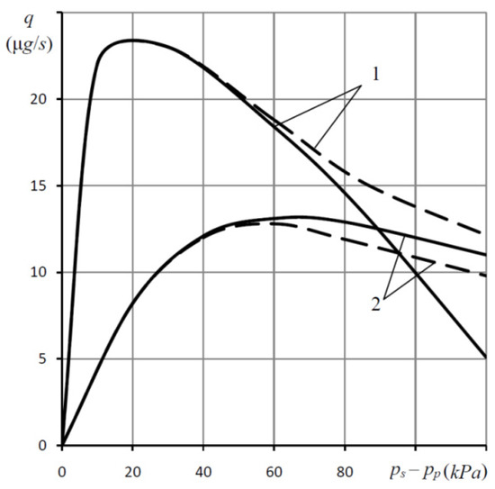
Figure 3. Comparison of the calculated (solid lines) and experimental (dashed lines) of the mass air flow dependences q through elastic openings from pressure difference p_s − p_p at r_s = 3.175 mm, 1—for r_p0 = 0.125 mm and δ = 2.64 mm, 2—for r_p0 = = 0.19 mm and δ = 1.14 mm.

The graph shows the theoretical (solid lines) and experimental (dashed lines) sensitivity curves of various-sized elastic orifices with Shore hardness A − 45 (E = 2.16 MN/m², ν = 0.5) at p_s = 238 kPa. The pressure difference p_s − p_p is plotted along the x-axis, and the mass flow q of gas through the orifice is plotted along the y-axis. The calculations used the formula

$$q=\frac{c_p\mathsf{\Gamma }{r}_p^2}{\sqrt{R_0{T}_0}}\mathsf{\Pi }\left(p_p,p_s\right)$$

where c_p = 0.85 the empirical coefficient of an orifice diaphragm [17], R₀ = 287 m²/(c² K) is the gas constant, T₀ = 293 K is the absolute temperature, Γ = 4.313 is the adiabatic constant of air [17].

It can be seen from Figure 3 that these curves have a complete qualitative and satisfactory quantitative agreement. Therefore, the described method can be used to a first approximation in the calculation of supports with an elastic orifice.

The discrepancy between the theoretical and experimental curves at large pressure drops (at large deformations of the elastic orifice) can be explained by the fact that with an increase in the strain, the error increases in the approximate formula (1), in Equations (2), (3), which do not take into account the changes in the functions ψ and u in the height of the elastic orifice, as well as in relation (9) based on Hooke’s law, which for rubber at large deformations gives a progressive error. At pressure drop values from low to moderate the discrepancy is no more than 15%–20%, which is quite acceptable. High values of the discrepancy appear only at excessively large differences, however, these modes are not of interest, because in this case the acceptable load of the bearing is way too low.

When calculating the compensating effect of an elastic orifice, the dimensionless input parameters varied in the region $P_s\in \left[1.5,6\right],$ $P_p\in \left[1.01,P_s\right],$ $R_{p0}\in \left[0.05,0.08\right],$ $\Delta \in \left[0.1,1.5\right],$ $\mathsf{\epsilon }\in \left[10,50\right],$ $\mathsf{\nu }\in \left[0.45,0.5\right].$

Figure 4 and Figure 5 shows the calculation results for the elastic orifice, showing that R_p substantially depends on Δ and ε and only slightly depends on ν.

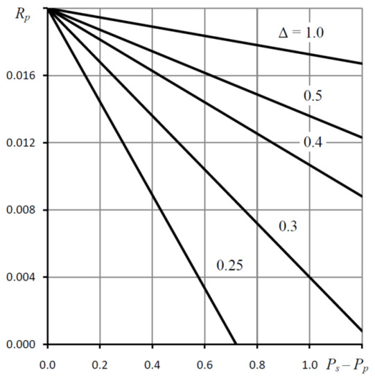
Figure 4. Dependences of R_p on P_s − P_p for various Δ; ε = 25, ν = 0.5, R_p0 = 0.02, ν = 0.5.

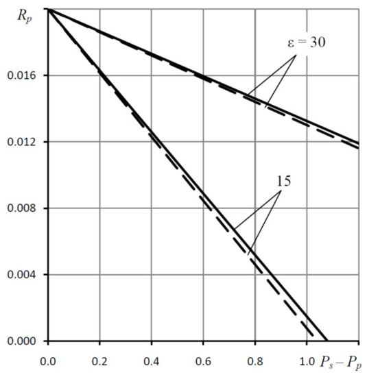
Figure 5. Dependences of R_p on P_s − P_p for various values of ε; ν = 0.5, Δ = 0.4, R_p0 = 0.02, solid lines— theory, dashed lines—experiment.

The working radius R_p is an almost linear function of the differential pressure, therefore, it can be approximated with the expression

$$R_p=R_{p0}\left[1-K_e\left(P_s-P_p\right)\right]$$

(18)

where K_e is the elastic ratio of the orifice.

Graphs of Figure 4 and Figure 5 and Equation (18) approximately determine the values of K_e. For the curves corresponding to ε = 15, we have approximate Equation (18), which implies that K_e ≈ 0.95. For the curves corresponding to ε = 30, a similar equation has the form $0.0119\approx 0.02\left(1-1.2K_e\right),$ whence it follows that K_e ≈ 0.34.

4. Bearing Mathematical Model

To model the bearings presented on Figure 1, we used a mathematical model of motion of a gas- static bearing with combined external throttling [23], which based on Reynolds differential equation [3,17], describes the pressure distribution in a thin lubricating gap, and uses the position of “continuous pressurization line” to replace discrete annular diaphragms with a continuous pressure function on the line of their locations [28].

The model takes into account the difference regarding the input throttling resistance, which is an elastic orifice. The dimensionless flow rate through this resistance is expressed by the formula

$$Q_p=A_p{R}_p^2\mathsf{\Pi }\left(P_s,P_p\right)$$

(19)

where the change in the radius of the passage of the elastic orifice is determined by formula (18).

4.1. Bearing Static Model

The static model will include two equations of equality of the flow rate Q_p through the elastic orifice and Q_k through the damping annular diaphragms, the flow rates Q_k and Q_h at the entrance to the bearing layer of the dimensionless thickness H, as well as the equation of force equilibrium of the movable element 2, connecting the bearing capacity W and the load F to the movable element

$$\{\begin{array}{l}{Q}_p-Q_k=0,\\ Q_k-Q_h=0,\\ W=F,\end{array}$$

(20)

where

$$Q_k=A_{k}H\mathsf{\Pi }(P_p,P_k)$$

(21)

$$Q_h=A_h\left(P_k^2-1\right)$$

(22)

$$W=\mathsf{\pi }\left[R_c^2\left(P_k-1\right)+2{\displaystyle \underset{R_c}{\overset{1}{\int }}R\left(P-1\right)dR}\right]$$

(23)

$$P(R)=\sqrt{\left(P_k^2-1\right)\frac{lnR}{ln{R}_c}+1}$$

(24)

$A_h=-1/\ln R_c$, Π is the Prandtl expiration function [23].

Obviously, the method of calculating the load characteristic H(F) used for conventional bearings, in which the input value is convenient to use H and the output F = W, is not suitable in this case, since, as will be shown below, this function can be multi-valued, i.e., several values of H may correspond to one value of F. Moreover, for certain values of this variable, the value of F may not be found.

Therefore, a parametric method was used to determine the load F and the gap H, as a function of pressure P_p

$$F=F(P_p),\hspace{1em}H=H(P_p).$$

When calculating the static characteristics, we used the boost pressure P_s, radius R_c, the tuning factors of the combined external throttling system χ, and the elastic ratio of the elastic orifice K_e.

The method for calculating static characteristics includes

–

determination of the “calculated point” parameters corresponding to the dimensionless thickness of the bearing layer H = 1,

–

calculation of flow rate Q(F) and load H(F) characteristics of the bearing.

In the “calculated point” mode, the coefficients A_k, A_p of expenses (21), (22) are determined. First, we calculate the coefficient A_h and determine the pressure P_k, P_p, corresponding to the value of the calculated clearance H = 1

$$P_k=\sqrt{1+\mathsf{\chi }\left(P_s^2-1\right)},\hspace{1em}{P}_p=\sqrt{P_k^2+\varsigma \left(P_s^2-P_k^2\right)},$$

then we calculate the coefficients

$$A_k=\frac{Q_h}{\mathsf{\Pi }\left(P_p,P_k\right)},\hspace{1em}{A}_p=\frac{Q_h}{\mathsf{\Pi }\left(P_s,P_p\right)}.$$

When calculating the flow and load characteristics, we sequentially set n_p pressure values $P_p\in \left[1,P_s\right]$ according to the formula $P_p=1+i_p\left(P_s-1\right)/n_p,\hspace{0.17em}$ $i_p=0,1,\dots ,n_p.$ For each of its values, we can find the flow Q_p according to formula (19).

The first two Equations (20) allow us to write a nonlinear equation for an unknown pressure $P_k\in \left[1,P_p\right]$ in the form

$$A_h{H}^3\left(P_k^2-1\right)-Q_p=0$$

(25)

where

$$H=\frac{Q_p}{A_k\mathsf{\Pi }(P_p,P_k)}$$

(26)

The solution of Equation (25) was found by the bisection method [27]. The integral in formula (23) of the bearing capacity W was calculated by the Simpson rule [18].

Bearing compliance is determined by the formula

$$K=-\frac{\partial H}{\partial F}$$

(27)

Equation (20) make it possible to establish the values of the elastic ratio K_e, at which the bearing reaches zero compliance (K = 0).

To determine the compliance of the bearing, we give the load F a small perturbation ΔF. The response will be disturbances ΔH, ΔP_k, ΔP_p, quantities H, P_k, P_p, respectively.

We write the system of Equation (20) with respect to disturbances in the matrix form

$$\left[\begin{array}{ccc}0& C_k& 0\\ C_{hh}& C_{hk}& -C_p\\ C_{kh}& C_{kk}& C_d\end{array}\right]\left[\begin{array}{c}\Delta H\\ \Delta P_k\\ \Delta P_p\end{array}\right]=\left[\begin{array}{c}1\\ 0\\ 0\end{array}\right]\Delta F$$

(28)

where

$$\begin{gathered} C_k=\frac{\partial W}{\partial P_k},C_{hh}=3A_h{H}^2\left(P_k^2-1\right),C_{hk}=2A_h{H}^3{P}_k,C_{kh}=A_k\mathsf{\Pi }\left(P_p,P_k\right),C_{kk}=A_{k}H\frac{\partial \mathsf{\Pi }\left(P_p,P_k\right)}{\partial P_k}, \\ {C}_{kp}=A_{k}H\frac{\partial \mathsf{\Pi }\left(P_p,P_k\right)}{\partial P_p},C_p=C_{p1}+K_e{C}_{p2},C_{p1}=A_p{R}_p^2\frac{\partial \mathsf{\Pi }\left(P_s,P_p\right)}{\partial P_p},C_{p2}=2A_p{R}_p\mathsf{\Pi }\left(P_s,P_p\right). \end{gathered}$$

Solving (28) by the Cramer rule [27], we obtain the formula for bearing compliance

$$K=-\frac{\Delta H}{\Delta F}=\frac{C_p\left(C_{kk}-C_{hk}\right)+C_{hk}{C}_{kp}}{C_k\left[C_p\left(C_{kh}-C_{hh}\right)+C_{hh}{C}_{kp}\right]}$$

(29)

Using (29), it is possible to set the value of the elastic ratio K_e, at which the bearing has zero compliance (K = 0). Most simply, this can be done for the "calculated point" mode H = 1. Using (19), (20), (22), (29), we find

$$\begin{gathered} R_p=\sqrt{\frac{A_k\mathsf{\Pi }\left(P_p,P_k\right)}{A_p\mathsf{\Pi }\left(P_s,P_p\right)}},C_p=\frac{C_{hk}{C}_{kp}}{C_{hk}-C_{kk}}, \\ {K}_{e0}=\frac{C_p-C_{p1}}{C_{p2}} \end{gathered}$$

(30)

In calculations it is sometimes convenient to use an inverse relationship

$$K_e\left(K\right)=\frac{1}{C_{p2}}\left[\frac{C_{kp}\left(C_{hk}-K{C}_k{C}_{hh}\right)}{K{C}_k\left(C_{kh}-C_{hh}\right)+C_{hk}-C_{kk}}-C_{p1}\right]$$

(31)

It has been found that for relatively large K_e, the bearing can lose stiffness. This is the case when the denominator (29) vanishes. It is easy to verify that this occurs when

$$K_{ed}=\frac{1}{C_{p2}}\left[C_{kp}{\left(1-\frac{C_{kh}}{C_{hh}}\right)}^{-1}-C_{p1}\right]$$

(32)

Note that the critical value of the elastic ratio K_e calculated by formula (32) occurs when R_p > 0, that is, when the orifice is still able to pass gas during deformation. It closes only when the pressure drop is too large and $K_e\ge \frac{1}{P_s-P_p}.$

4.2. Static Characteristics of the Bearing and Their Discussion

Figure 6 shows the load characteristics H(F) of an elastic orifice bearing for different values of elastic ratio K_e. All curves intersect at one point corresponding to the “calculated point” mode H = 1.

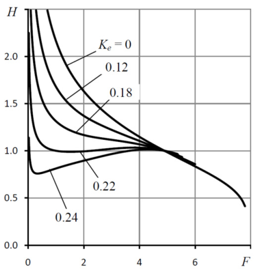
Figure 6. Load characteristics H(F) for various values of the elastic ratio K_e; P_s= 5, R_c = 0.5, χ = 0.48, ς = 0.3.

It can be seen that with increasing K_e, the curvature of the lines changes significantly. When K_e = 0, that is for the rigid orifice 3, the compliance of the bearing K is always positive. With increasing K_e in some parts of the load characteristic, the compliance decreases to zero (K = 0), which corresponds to infinite stiffness, and even a negative value (K < 0). So, at K_e = 0.22 and F ≈ 1.5, the bearing has zero compliance. At K_e = 0.22, one can find the region 0.35 < F < 4.4, in which the bearing has negative static compliance (K < 0).

Figure 7 shows graphs of expenditure flow rate dependencies Q(F). It is seen that with an increase in the coefficient K_e, the nature of the curves changes sharply. Comparison of graphs Figure 6 and Figure 7 shows that the less the compliance of the bearing, the lower the mass flow rate of air.

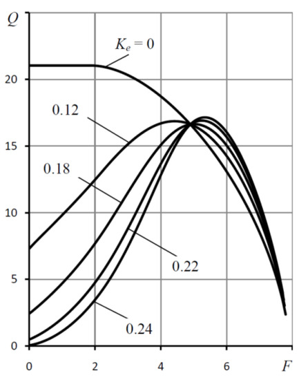
Figure 7. Flow rate characteristics Q(F) for various values of the elastic ratio K_e; P_s= 5, R_c = 0.5, χ = 0.48, ς = 0.3.

Figure 8 shows the curves of the dependence of the static compliance K on the coefficient ς of the setting of the damping annular diaphragms for the “calculated point” mode H = 1.

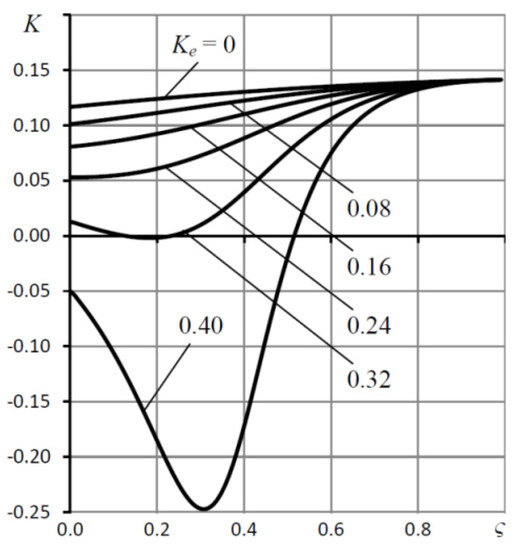
Figure 8. The dependences of the static compliance K on the coefficient ς for various values of the elastic ratio K_e; P_s= 5, R_c = 0.5, χ = 0.48.

This is explained by the fact that at low loads the pressure difference P_s − P_p is large, and as follows from formulas (18), (19) for K_e > 0, the diaphragm radius R_p will be small, and, therefore, the flow rate Q_p will be small. As the load F increases, the pressure difference P_s − P_p decreases and, consequently, the radius R_p and the flow rate Q_p increase, thereby providing an additional supply of lubricant to the bearing, which contributes to a more intensive decrease in bearing compliance K.

An analysis of the curves shows that the dependences K(ς) for the modes of positive compliance are monotonous in nature, while for zero and negative compliance they are unimodal in nature, where the minimum of the dependencies falls on a certain value of ς. Moreover, the smaller this minimum, the greater the corresponding ς.

Figure 9 shows the curves of the dependence of the elastic parameter K_e0 on the coefficient ς of the tuning of the damping annular diaphragms for the “calculated point” mode H = 1, at which the bearing has zero compliance. For smaller χ and ς, smaller K_e = K_e0 are required. At the same time, when setting to too small χ, there may be no modes in which the bearing reaches zero compliance.

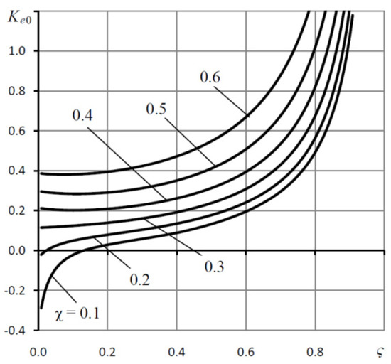
Figure 9. Dependences of the elastic parameter K_e0 on the coefficient ς for various values of the tuning coefficient χ; P_s = 5, R_c = 0.5.

Graphs of the dependence of the critical values of the elastic ratio K_ed(ς), at which the bearing loses its static stiffness, and, consequently, stability, are shown in Figure 10.

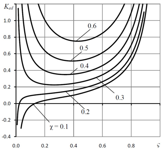
Figure 10. Dependences of the critical values of the elastic ratio K_ed on the coefficient ς for various values of the tuning coefficient χ; P_s = 5, R_c = 0.5.

The K_ed values determined by formula (31) give the upper boundary on the admissible values of the elastic ratio K_e = K_ed. For K_e > K_ed, the bearing is also statically unstable.

5. Bearing Dynamic Model

The mathematical model of the bearing dynamics is based on a bearing motion model with combined external throttling [23]. The only difference is that the formula for the deviation of the Laplace transform of the gas flow through the throttling simple diaphragm is replaced with the corresponding flow formula through the elastic orifice, which has the form

$$\begin{gathered} \overline{\Delta Q_p}=A_{pp}\overline{\Delta P_p}, \\ \hspace{1em}{A}_{pp}=A_P{R}_p\left[R_p\frac{\partial \mathsf{\Pi }\left(P_s,P_p\right)}{\partial P_p}+2K_e\mathsf{\Pi }\left(P_s,P_p\right)\right] \end{gathered}$$

where R_p, P_p are static parameters.

5.1. Method for Determining the Transfer Function Coefficients of Dynamic Bearing Compliance

In the calculations, a new method was used to determine the criteria for the quality of bearing dynamics, the essence of which is described below.

The transfer function (TF) of the dynamic compliance of the bearing, as a system of automatic control and regulation can be represented in the form

$$K(s)=\frac{\overline{\Delta H}}{\overline{\Delta F}}=\frac{b_0+b_{1}s+b_2{s}^2+\dots +b_m{s}^m}{1+a_{1}s+a_2{s}^2+\dots +a_n{s}^n}$$

(33)

where n > 0, m > 0, n > m, s is the Laplace transform variable [29].

The denominator (33) is the characteristic polynomial (CP) of a linear dynamic system with distributed parameters, the use of which in the study of its dynamics quality allows us to determine the stability margin and evaluate the system’s speed from the roots of the characteristic equation [18,29].

For a system with distributed parameters, it is necessary to use a method that would ensure its presentation in the form (33) based on the calculation of the criteria of stability margin and speed of devices with a predetermined accuracy.

The representation of the TF in the form of (33) falls under the classical problem of rational interpolation [30], the solution of which, however, does not provide an exhaustive answer to the question of the accuracy of the system stability criteria obtained by root methods using the characteristic equation, because the value of the degree of CP is unknown in advance.

Existing methods of linear interpolation are based on solving a linear system of equations with respect to coefficients (33), which contains n + m equations [30]. Such systems can be solved using general methods, for example, the Gauss–Jordan method, which has a cubic order of complexity (n + m)³ (hereinafter, the order of complexity of the computational method means the time complexity of the algorithm that implements it [30,31]). For large n and m, this can entail a significant expenditure of computer time in the process of multi-parameter optimization of a dynamic system.

This article presents a quick method to find the coefficients (33). It is based on solving systems of linear equations of a special form of a substantially smaller order, which allows one to find their solution using fast methods with a quadratic order of complexity m(n + m), which contributes to a significant acceleration of the optimization procedure for dynamic systems. If it is required to find only CP coefficients, then the order of complexity of the method is n².

When conducting rational interpolation, the degrees n and m of polynomials (33) should be known. However, their acceptable values can be obtained only on the basis of satisfactory accuracy in determining the quality criteria of the dynamics of the system.

If it is impossible to determine the values of these parameters without calculating the mentioned criteria, then finding their difference is not difficult.

Indeed, if a_n ≠ 0 and b_m ≠ 0, then the infinite limit

$$s^{p}K(s)\to \frac{b_m}{a_n}\ne 0$$

(34)

where p = n − m.

Usually, the difference p is calculated in several units, more often p = 1 or 2, therefore, you can find this limit and p can be fast enough.

We set the value of m, define n = m + p and find the coefficient

$$b_0=K(0).$$

We rewrite (1) in the form

$$a_1+a_{2}s+\dots +a_n{s}^{n-1}+\mathsf{\Gamma }(s)\left(b_1+b_{2}s+\dots +b_m{s}^{m-1}\right)=\mathsf{\Lambda }(s)/s$$

(35)

where

$$\mathsf{\Gamma }(s)=\frac{-1}{K(s)},\mathsf{\Lambda }(s)=-b_0-\mathsf{\Gamma }(s).$$

Equation (35) contains k = n + m unknown coefficients.

We calculate $e=exp\left(-\frac{2\mathsf{\pi }i}{k}\right),$ where i is the imaginary unit.

Put $s_1=1$, and find $s_j=e\hspace{0.17em}{s}_{j-1}$, $j=2,3,\dots ,k$ ${\mathsf{\Psi }}_j=K\left(s_j\right),$ ${\mathsf{\Gamma }}_j=\mathsf{\Gamma }\left(s_j\right)$, $\hspace{0.17em}{\mathsf{\Lambda }}_j=\mathsf{\Lambda }\left(s_j\right),$ $j=1,2,\dots ,k.$

Note that $s_j=\hspace{0.17em}{s}_{k+1-j}^{\ast },\hspace{0.17em}j=1,2,\dots ,k,$ therefore, $K\left(\hspace{0.17em}{s}_{k-j+1}\right)=K^{\ast }\left(\hspace{0.17em}{s}_j\right),\hspace{0.17em}$ it allows us to reduce the computation and find ${\mathsf{\Gamma }}_j,{\mathsf{\Lambda }}_j$ in [(k + 1)/2] access to the TF.

Substituting s = s_j, (j = 1, 2, …, k) in sequence (35), we obtain a system of linear equations for unknown coefficients (33)

Mx = y

(36)

where

$$\begin{gathered} M=\left[\begin{array}{cccccc}{s}_1& s_1& s_1& \dots & {\mathsf{\Gamma }}_1{s}_1& \dots \\ s_1& s_2& s_3& \dots & {\mathsf{\Gamma }}_2{s}_1& \dots \\ s_1& s_3& s_5& \dots & {\mathsf{\Gamma }}_3{s}_1& \dots \\ \dots & \dots & \dots & \dots & \dots & \dots \\ s_1& s_k& s_1& \dots & {\mathsf{\Gamma }}_k{s}_1& \dots \end{array}\right], \\ x=\left[\begin{array}{c}{a}_1\\ a_2\\ \dots \\ b_{m-1}\\ b_m\end{array}\right],y=\left[\begin{array}{c}{\mathsf{\Lambda }}_1/s_1\\ {\mathsf{\Lambda }}_2/s_2\\ \dots \\ {\mathsf{\Lambda }}_{k-1}/s_{k-1}\\ {\mathsf{\Lambda }}_k/s_k\end{array}\right]. \end{gathered}$$

We represent the matrix of the system in the form

M = ΦU

(37)

where U is the matrix, Φ is the matrix of the discrete Fourier transform [32]

$${\mathsf{\Phi }}_{i,j}=S(i,j)$$

where

$$\begin{array}{l}S(i,j)=s_{1+q((i-1)(j-1))},\hspace{0.17em}i=1,2,\dots ,k-1;\hspace{0.17em}j=1,2,\dots ,k-1,\\ q(x)=x\hspace{0.17em}\mathrm{mod}\hspace{0.17em}k.\end{array}$$

Its inverse matrix is determined by the formula

$${\mathsf{\Phi }}_{i,j}^{-1}=\frac{1}{k}\overline{S}(i,j).$$

Multiplying Φ⁻¹ by (37), we bring the system (35) to the form

Ux = z

(38)

where $U={\mathsf{\Phi }}^{-1}M,$ $z={\mathsf{\Phi }}^{-1}y.$

For m > 0, the matrix U has a cellular structure of the form

$$U=\left[\begin{array}{cc}E& C\\ 0& D\end{array}\right].$$

where E and 0 are the identity and zero matrices of size $n\times n$ and $m\times n$, C and D are Toeplitz matrices of size $n\times m$ and $m\times m$, respectively [31].

Indeed, the blocks of matrices Φ⁻¹ and M cells are mutually inverse matrices of the discrete Fourier transform, therefore, their product will give the identity matrix E. Elements of the block of cells are obtained by multiplying the rows of the matrix Φ⁻¹ and the columns of the matrix M, which are also elements of the direct and inverse matrices Fourier transform. The sums of their products, giving off-diagonal elements of the identity matrix, will be zeros by analogy with the way this holds for the zero elements of the block E located above them.

The nature of the matrices A and B is explained by the fact that the elements of the columns of the matrix M for j > n are formed by sums of products of displaced elements of the matrix Φ and the elements of vector Γ that are different from unity. In such cases, their scalar products yield Toeplitz matrices [31].

From Equations (37) and (38) it follows that for m > 0 the vector b of the coefficients of the TF (33) satisfies the system of equations

Db = d

(39)

where d is a vector.

Compared to the original Equation (35) of order k = n + m, Equation (39) has a significantly lower order of m < k/2. Therefore, the solution for it can be obtained much faster.

Equation (39) is a standard problem with an asymmetric Toeplitz matrix of a special form [33], which can be solved both using general methods, for example, the Gauss–Jordan method [34], the complexity of which is proportional to m³, and using special fast methods taking into account the features of Equation (39) and having complexity proportional to m². The latter include the methods described in [33,34].

Elements of the matrix C can be expressed in terms of the vector l

$$C_{i,j}=l_{q(k+i-j)},\hspace{1em}i=1,2,\dots ,n;\hspace{1em}j=1,2,\dots ,m.$$

With this in mind, we can dispense with the matrix C and, using the solution of system (10), quickly find the CP coefficients using the complexity nm formula

$$a_i=l_i-{\displaystyle \sum _{j=1}^m{l}_{q(k+i-j)}\hspace{0.17em}{b}_j},\hspace{1em}i=1,2,\dots ,n.$$

With this in mind, the total complexity order of this method for finding the coefficients (33) is m(n + m).

5.2. Quality Criteria for Bearing Dynamics

To assess the quality of the dynamics of linear systems, root criteria are often used [29]:

–

degree of stability η = Max Re{s_i}, where s_i are the zeros of the characteristic polynomial of the dynamical system, which is the polynomial denominator of the TF (33),

–

damping of oscillations over a period $\mathsf{\xi }=100[1-Exp\left(-\left|2\mathsf{\pi }\mathsf{\beta }/\mathsf{\eta }\right|\right)]\hspace{0.17em}\%$, where β is the imaginary part of the root of the characteristic equation with the largest real part.

The degree of stability η characterizes the speed of the system, that is, the rate of attenuation of its free oscillations.

The criterion ξ of damping of oscillations over a period can be applied to the estimation of the system stability margin. The smaller ξ, the greater the transient response will have an oscillation, and the system will have a smaller margin of stability. It is believed that a dynamic system is well damped if ξ ≥ 90% [29].

At the beginning, using the algorithm for calculating the values of the transfer function, the degree difference is determined by the TF polynomial p = n − m based on (34).

Further calculations are carried out using the following iterative process.

Step 1.

Put i= 1 and m = 1, η₀ = inf, ξ₀ = inf, where inf is a large number (for example, inf = 10¹⁰), set the accuracy of determining the degree of stability ε_η and the damping of oscillations for the period ε_ξ.

Step 2.

Calculate n = p + m and, after performing rational interpolation find the vector a of the CP coefficients.

Step 3.

Determine the roots of the characteristic equation, find among them the root with the largest real part and calculate the criteria η_i and ξ_i.

Step 4.

Verify that the iterative process converges to a solution

$$\left|{\mathsf{\eta }}_i-{\mathsf{\eta }}_{i-1}\right|<{\epsilon }_{\eta },\left|{\mathsf{\xi }}_i-{\mathsf{\xi }}_{i-1}\right|<{\mathsf{\epsilon }}_{\mathsf{\xi }}.$$

Step 5.

If conditions (12) are fulfilled, then the quality criteria of the system dynamics are determined with the required accuracy, otherwise the process should be continued. To do this, increase the values of the iteration counter i and degree m by one and go to step 2.

The method described above was used to calculate the quality criteria of the dynamics of the bearing under consideration.

5.3. Bearing Dynamic Characteristics and Discussion

Among the parameters that do not affect the static characteristics, but affect the dynamic characteristics of the bearing, are the “compression number” σ and the volume of the intermediate cavity V_p [23]. The influence of these parameters is of particular interest, because they are a resource to optimize the quality of a dynamic system.

Table 1 shows the results of bearing optimization according to the performance criterion, which consisted in finding such pairs (σ, V_p) whose values deliver the maximum degree of stability η. Optimization was carried out for the values of other input parameters: P_s = 5, R_c= 0.5, χ = 0.48, ς = 0.3, H = 1. The parameter iK was varied, with the help of which the static compliance K was calculated by the formula

$$K=iK·K_0,$$

where K₀ is the static compliance of the bearing corresponding to hard orifice 3 (K_e = 0). Corresponding K values of the coefficient K_e were calculated by the formula (30).

Table 1. Optimum bearing parameters.

iK	K	Ke	η	σ	Vp
1.0	0.127	0	0.301	11.6	15.4
0.5	0.064	0.342	0.288	13.2	5.9
0	0	0.320	0.278	13.2	6.6
−0.5	−0.064	0.382	0.272	13.9	4.2
−1.0	−0.127	0.378	0.274	14.0	4.3
−1.5	−0.264	0.401	0.264	15.3	3.2

An analysis of the calculation results showed that for each set of source data there is exactly one pair of values of the parameters σ, V_p that deliver the maximum performance criterion η. From Table 1 it follows that with a decrease in compliance, the optimal σ tends to increase, while the optimal V_p tends to decrease. With an increase in K_e, the performance of the bearing decreases somewhat, but it remains stable even with negative values of K that are in absolute value superior to those of a conventional bearing (K_e = 0).

A detailed idea of the influence of the parameters σ, V_p on the degree of stability is given by the graph curves of Figure 11, which are constructed for the same initial data and K_e = 0.32, at which the bearing has zero static compliance (K = 0).

Figure 11. Dependences of the degree of stability η on the “compression number” σ for various values of the volume V_p.

The graphs confirm the conclusion that the dependences η(σ) and η(V_p) are extreme. It can be seen that for the regime of zero compliance, it is necessary to choose the values σ > σ_min, where σ_min is the value of the parameter σ at which the system reaches the stability boundary (η = 0).

For σ < σ_min, the system is unstable, and for σ > σ_min the stability region is divided into two parts σ_min < σ < σ_opt and σ > σ_opt, where σ_opt is the value of the parameter σ at which the function η(σ) reaches its maximum.

It was found that in the first part of this region, the transient characteristics are always oscillatory in nature, and in the second, they can be both oscillatory and aperiodic.

This follows from the analysis of graphs in Figure 12, where the dependences of the decay criterion for the period ξ on the compression number σ are presented. For V_p < V_popt, the criterion ξ indicates the oscillatory nature of the transients (ξ < 100%), where V_p opt are the values of the parameter Vp at which the function η(V_p) reaches its maximum. The graphs show that for V_p < V_{p opt} all the curves, regardless of the value of σ, indicate the vibration nature of the transients (ξ < 100%), for V_p > V_popt the transients become aperiodic (ξ = 100%). It is also seen that with an increase in V_p, the range of aperiodicity of the transient characteristics expands, that is, an increase in the volume of V_p contributes to an increase in the dynamic stability margin of the bearing as a dynamic system.

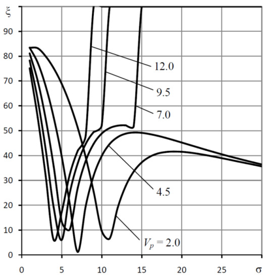
Figure 12. Dependences of criterion ξ on the “compression number” σ for various values of the volume V_p.

The data obtained allow us to give recommendations on the choice of values of the parameters σ and V_p. The values of σ and V_p should be considered the best, which are slightly larger than the optimal σ_opt and V_popt. For example, for the mode of zero static compliance K = 0, σ = 14 and V_p = 7 will be the best. In this case, the bearing will have close to maximum speed and an aperiodic nature of the transition characteristics.

6. Conclusions

A mathematical model of statics and dynamics of a thrust gas-static bearing with an elastic orifice was formulated, a model for the deformation of an elastic orifice and a method to calculate the radius of its throttling diaphragm are proposed, a fast numerical method to calculate the quality indicators of the dynamics of a linear system with distributed parameters was developed, methods for determining the static and dynamic characteristics of the bearing were developed.

Calculations using the proposed model of elastic orifice deformation showed that its characteristics have full qualitative and satisfactory quantitative agreement with the results of experiment [22]. The flaws of the model were revealed and it was concluded that the proposed model and the method described can be used to a first approximation to calculate the radius of the supply diaphragm of the elastic orifice. The results of the study of the deformation of the elastic orifice are the basis for the model of the static and dynamic state of the bearing.

A formula was derived that allows one to calculate the value of the elastic ratio at which the bearing reaches zero compliance, and a formula to calculate the value of this parameter, at which the bearing loses its static stability.

The use of the fast numerical method to calculate the bearing dynamics quality criteria made it possible to repeatedly increase the speed of the multi-parameter design optimization algorithm by the performance criterion. A numerical experiment showed that, compared with the previously used method, the speed of the algorithm increased by about 12 times.

It was shown that the use of an elastic orifice allows a multiple reduction of positive compliance of the bearing, and also allows reduction of the compliance of the bearing to zero and even negative values.

An analysis of the quality criteria of structural dynamics confirms that with an optimal choice of the compression number σ and the volume of the inter-throttle chamber V_p of the throttle chamber, the bearing can provide high speed and a guaranteed stability margin, while keeping the transition characteristics non-oscillatory.

References

- Bushuev, V.V.; Sabirov, F.S. Directions of development of the world machine tool industry. Bull. Moscow State Tech. Univ. STANKIN 2010, 1, 24–30. [Google Scholar]
- Kawada, S.; Miyatake, M.; Yoshimoto, S.H.; Stolarski, T. Static and dynamic characteristics of a downsized aerostatic circular thrust bearing with a a single feed hole. Precis. Eng. 2019, 60, 448–457. [Google Scholar] [CrossRef]
- Al-Bender, F. On the modelling of the dynamic characteristics of aerostatic bearing films: From stability analysis to active compensation. Precis. Eng. 2009, 33, 117–126. [Google Scholar] [CrossRef]
- Belforte, G.; Colombo, F.; Raparelli, T.; Trivella, A.; Viktorov, V. High Speed Rotors on Gas Bearings: Design and Experimental Characterization. In Tribololgy in Engineering; Hasim, P., Ed.; InTech: Rijeka, Croatia, 2013. [Google Scholar] [CrossRef]
- Cui, C.; Ono, K. Theoretical and Experimental Investigation of an Externally Pressurized Porous Annular Thrust Gas Bearing and Its Optimum Design. ASME J. Tribol. 2016, 119, 486–492. [Google Scholar] [CrossRef]
- Mizumoto, H.; Matsubara, T.; Hata, N.; Usuki, M. Zero-compliance aerostatic bearing for an ultra-precision machine. Precis. Eng. 1990, 12, 75–80. [Google Scholar] [CrossRef]
- Renn, J.C.; Hsiao, C.H. Experimental and CFD Study on the Mass Flow-rate Characteristic of Gas through Orifice-type Restrictor in Aerostatic Bearings. Tribol. Int. 2004, 37, 309. [Google Scholar] [CrossRef]
- Chen, M.F.; Lin, Y.T. Static Behavior and Dynamic Stability Analysis of Grooved Rectangular Aerostatic Thrust Bearings by Modified Resistance Network method. Tribol. Int. 2002, 35, 329. [Google Scholar] [CrossRef]
- Lin, W.J.; Khatait, J.P.; Lin, W.; Li, H. Modelling of an Orifice-type Aerostatic Thrust Bearing. In Proceedings of the 9th International Conference on Control, Automation, Robotics and Vision, Singapore, Singapore, 5–8 December 2006; IEEE: Piscataway, NJ, USA, 2006. [Google Scholar] [CrossRef]
- Stout, K.J.; Barrans, S.M. The Design of Aerostatic Bearings for Application to Nanometre Resolution Manufacturing Machine Systems. Tribol. Int. 2000, 33, 803. [Google Scholar] [CrossRef]
- Fourka, M.; Bonis, M. Comparison Between Externally Pressurised Gas Thrust Bearings with Different Orifice and Porous Feeding System. Wear 1997, 210, 311–317. [Google Scholar] [CrossRef]
- Raparelli, T.; Viktorov, V.; Colombo, F.; Lentini, L. Aerostatic thrust bearings active compensation: Critical review. Precis. Eng. 2016, 44, 1–12. [Google Scholar] [CrossRef]
- Stout, K.J.; El-Ashakr, S.; Ghasi, V.; Tawfik, M. Theoretical Analysis of Two Configurations of Aerostatic Flat Pad Bearings using Pocketed Orifice Restrictors. Tribol. Int. 1993, 26, 265. [Google Scholar] [CrossRef]
- Kodnyanko, V.A.; Kurzakov, A.S. Improving the dynamic performance of a circular gas-static thrust bearing with annular diaphragms. Assem. Mech. Eng. Instrum. Mak. 2017, 18, 4–10. [Google Scholar]
- Aguirre, G.; Al-Bender, F.; Van Brussel, H. A multiphysics model for optimizing the design of active aerostatic thrust bearings. Precis. Eng. 2010, 34, 507–515. [Google Scholar] [CrossRef]
- Kodnyanko, V.A. Compliance of a gas-dynamic bearing with an elastic displacement compensator. J. Sib. Fed. Univ. Tech. Technol. 2017, 10, 657–663. [Google Scholar] [CrossRef]
- Pinegin, S.V.; Tabachnikov, Y.B.; Sipenkov, I.E. Statistical and Dynamic Characteristics of Gas-Static Supports; Science: Moscow, Russia, 1982; p. 264. [Google Scholar]
- Riley, K.F.; Hobson, M.P.; Bence, S.J. Mathematical Methods for Physics and Engineering; Cambridge University Press: Cambridge, UK, 2010; p. 45. [Google Scholar]
- Laub, J.H. Elastic Orifices for Gas-Lubricated Bearings. J. Basic Eng. 1960, 82, 980–982. [Google Scholar] [CrossRef]
- Laub, J.H.; Batsch, F. Elastic Orifices as Pneumatic Logic Elements. In JPL Research Summary 36-12; Jet Propulsion Laboratory: Pasadena, CA, USA, 1962; Volume 1, p. 35. [Google Scholar]
- Stanford Research Institute. Elastic Orifices for Gas Bearings; National Aeronautics and Space Administration: Washington, DC, USA, 1965.
- Newgard, P.M.; Kiang, R.L. Elastic orifices for pressurized gas bearings. ASLE Trans. 1966, 3, 311–317. [Google Scholar] [CrossRef]
- Kodnyanko, V.A.; Shatokhin, S.N. Theoretical Study on Dynamics Quality of Aerostatic Thrust Bearing with External Combined Throttling. FME Trans. 2020, 46, 342–350. [Google Scholar] [CrossRef]
- Kodnyanko, V.A. Characteristics of a gas-static thrust bearing with an active displacement controller. Mosc. J. Metal Cut. Mach. Tools 2005, 9, 32–34. [Google Scholar]
- Ponomarev, S.D. Strength Calculations in Mechanical Engineering; Mashgiz: Moscow, Russia, 1988. [Google Scholar]
- Timoshenko, S.P. Strength of Materials, Part 1 and Part 2; Krieger Publishing Company: Malabar, FL, USA, 1983; p. 1010. [Google Scholar]
- Isaacson, E.; Keller, H.B. Analysis of Numerical Methods; Dover Publications: Mineola, NY, USA, 1994; p. 576. [Google Scholar]
- Stepanyants, L.G.; Zablotsky, N.D.; Sipenhov, I.E. Method of theoretical research of externally pressurized gas-lubricated bearings. J. Lubr. Technol. 1969, 91, 166–170. [Google Scholar] [CrossRef]
- Besekersky, V.A.; Popov, E.P. Theory of Automatic Control Systems; Profession: St. Petersburg, Russia, 2002; p. 752. [Google Scholar]
- Press, W.H.; Teukolsky, S.A.; Vetterling, W.T.; Flannery, B.P. Rational Function Interpolation and Extrapolation. In Numerical Recipes in C; Cambridge University Press: Cambridge, UK, 1994. [Google Scholar]
- Heinig, G.; Rost, K. Efficient Inversion Formulas for Toeplitz-Plus-Hankelmatrices Using Trigonometric Transformations. Structured Matrices in Mathematics. In Contemporary Mathematics; Computer Science, and Engineering II; American Mathematical Society: Providence, RI, USA, 2001; Volume 281, pp. 247–264. [Google Scholar]
- Smith, S.W. The Discrete Fourier Transform. In The Scientist and Engineer’s Guide to Digital Signal Processing; California Technical Publishing: San Diego, CA, USA, 1999. [Google Scholar]
- Golub, G.H.; Van Loan, C.F. Matrix Computations; John Hopkins Studies in the Mathematical Sciences; John Hopkins University Press: Baltimore, MD, USA, 1996. [Google Scholar]
- Blahut, R.E. Fast Algorithms for Signal Processing; Cambridge University Press: Cambridge, UK, 2010; p. 469. [Google Scholar] [CrossRef]
© 2020 by the authors. Licensee MDPI, Basel, Switzerland. This article is an open access article distributed under the terms and conditions of the Creative Commons Attribution (CC BY) license (http://creativecommons.org/licenses/by/4.0/).