1. Introduction
An extremely important contribution to the understanding of indentation testing, and other related contact mechanics-based testing, was presented by Johnson [
1,
2]. In summary, it was concluded in these studies that the mechanical behavior of global indentation properties can be correlated based on a single parameter (here and below named the Johnson parameter) and that the mechanics of the indentation problem is very much dependent on the combination of the material and geometrical quantities included in this parameter. The Johnson parameter will be discussed in more detail in the next section.
The analyses by Johnson are pertinent to initially stress-free materials. Later it has been shown [
3,
4,
5] that it is possible to also include indentation of residually stressed materials in Johnson’s single parameter correlation. A very important conclusion was presented by Pharr et al. [
6,
7], saying that indentation hardness is invariant of residual stresses for metals and alloys. This is not so however for another global indentation quantity: the relative contact area. This feature can be used for determining residual stresses [
8,
9,
10,
11,
12].
The results of the Pharr et al. [
6,
7] study is concerned with metals and alloys where plasticity dominates the deformations around the indentation contact zone. However, this is not so in the case of such materials as ceramics and polymers where elastic and plastic deformations are of equal magnitude at the indent. In such a situation, residual stresses do indeed influence hardness values [
13,
14] and consequently this quantity could be used for residual stress determination.
The results in [
13,
14] can be summarized as follows:
When elastic deformations around the contact region are in the same order as plastic ones; then the hardness is dependent on residual stresses.
In case of equi-biaxial surface stresses, correlation with the Johnson parameter is accurate and produces a general relation with corresponding stress-free results when residual stresses are appropriately accounted for.
In case of uniaxial surface stresses, correlation with the Johnson parameter is not good and in such a situation; the hardness variation is not a good tool for an experimental determination of residual stresses.
Obviously, there is a fundamental difference in mechanical indentation behavior between equi-biaxial and uniaxial surface stresses. Accordingly, it is of interest to investigate this feature also for other types of surface stress fields (deviating from equi-biaxial or uniaxial). This is also the aim of the present investigation.
In doing so, previous finite element results [
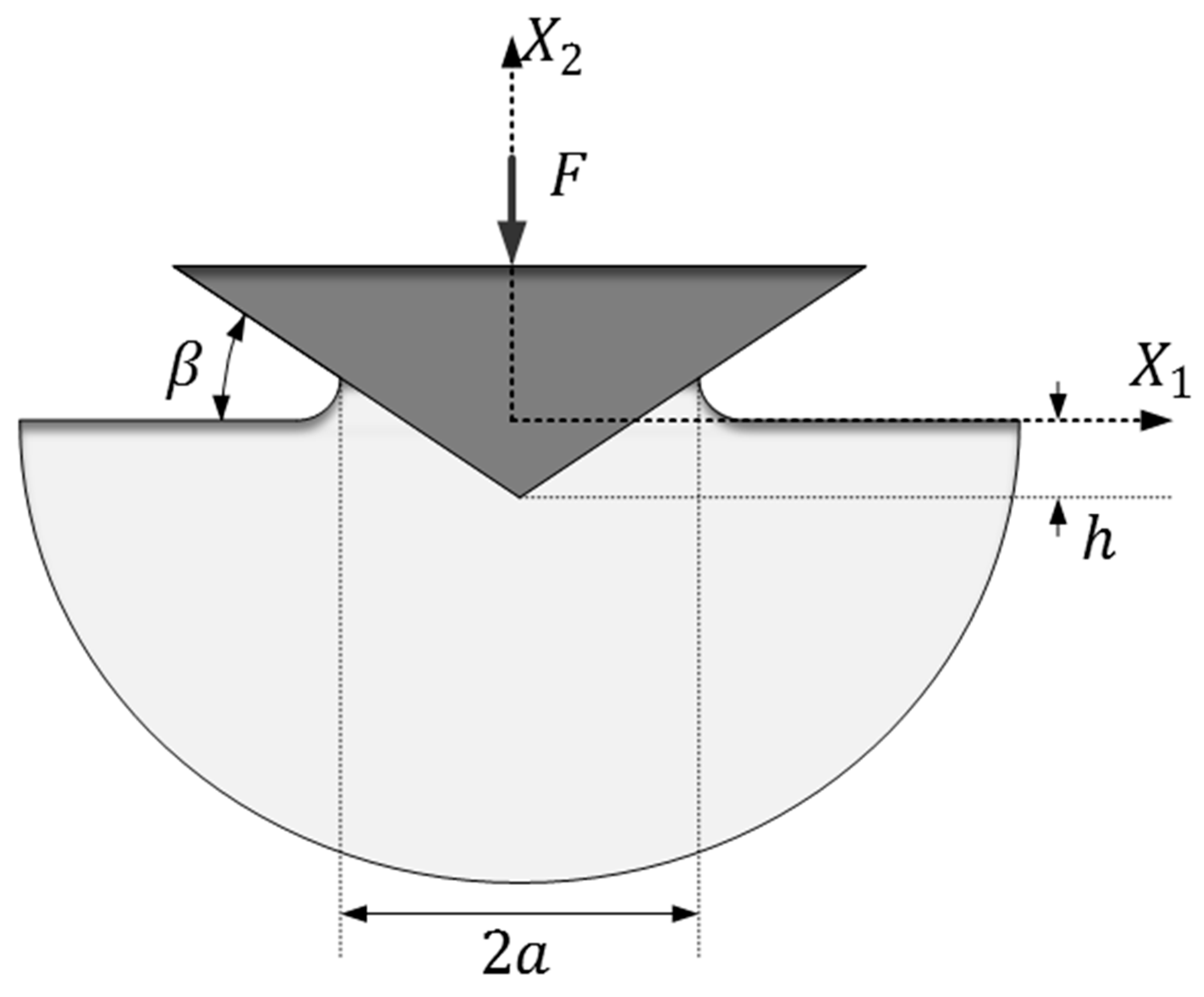
12] and additional finite element simulations performed presently will be revisited within the question at issue above. For simplicity, but not out of necessity, only cone indentation (
Figure 1) of elastic-perfectly plastic materials is considered. Strain-hardening effects could easily be incorporated into the analysis based on the representative strain concept [
15].
Finally, it should be mentioned that the discussion above has been restricted to features related to sharp indentation. This is the most straightforward interpretation of the results and this study will be entirely devoted to such indenter geometry. Having said this, it is important to emphasize that quite a few important contributions concerning spherical and other blunt indenters (including cones with a rounded tip), as a tool for residual stress determination, has been previously presented [
16,
17,
18,
19,
20], just to mention a few.
2. Theoretical Background
The analysis by Johnson [
1,
2] defined the fundamentals for a general analysis of indentation testing. Specifying to sharp indentation on classical elastoplastic materials a general correlation parameter could be defined as:
In Equation (1),
E is the Young’s modulus and
ν is Poisson’s ratio, β is the angle between the (sharp) indenter and the undeformed surface, and
σrep is the material flow stress at a representative value of the equivalent (accumulated) plastic strain
εp. Based on the parameter
Λ three regions or levels of contact behavior can be defined. These levels, as shown in
Figure 2, are:
Level I: Dominating elastic deformations, i.e., low indentation load, where an elastic contact analysis is sufficient.
Level II: Elastic and plastic deformations are of equal magnitude.
Level III: Plastic deformations are dominating in the contact region.
In level II, it was determined by Johnson [
1,
2] that in this region
while in level III, Tabor [
21] showed that at sharp indentation
For a Vickers indenter
C ≈ 3 and
εp ≈ 0.08 (Tabor [
2]) and for a cone indenter C ≈ 2.54 and
εp ≈ 0.11 (Atkins and Tabor [
22]). The latter case is specified for a cone indenter with an angle of 22° between the indenter and the undeformed surface being at issue here, see
Figure 1. In Equations (2) and (3),
H is the material hardness defined as the average contact pressure between indenter and material.
At level III conditions, and also at substantial parts of the level II region in
Figure 2, the hardness is, as stated above, invariant of residual stresses. However, this is not so for the relative contact area:
where
A (true contact area) and
Anom (nominal contact area) are projected areas (
Figure 1). This quantity can indeed be related to an equi-biaxial residual stress
σres according to:
where
c2(
σres = 0) is the value on the relative contact area at indentation of a virgin (unstressed material) and
F is a constant that takes on different values at tension and compression. For simplicity but not for necessity ideal plasticity, with a yield stress
σy, is here assumed. The Equation (5) was originally proposed by Rydin and Larsson [
5] based on the similar mechanical behavior between contact induced stresses in an unstressed material or contact induced stresses in a material with a properly chosen apparent initial yield stress. Rydin and Larsson [
5] suggested an apparent yield stress:
(
σy being the initial yield stress of the material) in
Λ in Equation (1), according to:
This makes it possible to rely on a universal
c2-curve, shown schematically in
Figure 2, regardless if residual stresses are present or not. This curve can be used to determine
σres when
c2(
σres = 0) is known.
When elastic and plastic deformations are of equal size, invariance of hardness is lost. This is pertinent to the linear variation regime of the normalized hardness,
H/
σy, in
Figure 2. It was recently shown by Larsson [
13] that it is possible to correlate the influence from residual stresses on hardness values, in essentially the same way as for the relative contact area
c2, when the residual stresses are equi-biaxial. This correlation is, again as for
c2, based on Equations (6) and (7) and is explicitly shown in
Figure 3, and obviously very good agreement with a universal curve is achieved. Corresponding results [
14] were then presented for a uniaxial stress state and unfortunately, correlation with a universal curve was not good.
Based on the results in [
13,
14], it can be concluded that the influence from residual stresses on the indentation hardness is quite different in an equi-biaxial situation compared to a uniaxial situation. This indicates that a more general approach to the problem is of substantial interest and this will be attempted presently. In doing so, a more general residual surface stress state will be investigated.
3. Numerical Analysis
In this section, the present finite element simulations of the cone indentation problem are described. It is then important to emphasize that, due to the fact that uniaxial residual stress states are considered, axisymmetric conditions are lost and a full three-dimensional (3D) solution has to be sought for. Similar analyses have been previously performed [
13] and, accordingly, concerning details of the numerical approach of this article is referred to.
Quasi-static cone indentation of elastic-ideally plastic pre-stressed materials is analyzed here. Frictionless contact is assumed in all simulations. Concerning the constitutive description, the rate-independent Prandtl-Reuss equations for classical plasticity are relied upon accounting for large deformations. Ideally, plastic conditions are assumed throughout the entire analysis and accordingly plastic deformation is initiated and maintained when the equivalent stress.
When elastic loading or unloading is an issue, a hypoelastic formulation of Hooke’s law is used.
The material hardness is, as stated above, defined as the average contact pressure during loading according to:
where
F is the indentation load and
A is the projected contact area. In this context, it should be mentioned that if the residual stresses are homogeneous as assumed presently, the problem is self-similar with no characteristic length and, as a result of global indentation properties, such as hardness and relative contact area, are independent of indentation depth.
As indicated above, the residual stress field is defined by the principal residual surface stresses σ1 and σ2. For a general surface stress state, the contact area will become ellipsoidal with semi-axes a1 ≠ a2. Accordingly, a three-dimensional finite element analysis is required at uniaxial residual loading. Clearly, since surface residual stresses are at issue the principal stress σ3 = 0.
The boundary value problem schematically outlined above was solved using the multi-purpose finite element program ABAQUS [
23]. The full indentation procedure, starting at initial contact between indenter and material, was modelled. Approximately 100,000 eight-node hybrid solid elements (element type C3D8H in ABAQUS [
23]) were used to discretize the material while the conical indenter was assumed to be rigid. Due to existing symmetries only one quarter of the material needs to be modelled. The resulting finite element mesh is shown in
Figure 4, where for clarity only the mesh details close to the contact region is shown. Residual (applied) stresses are enforced by prescribed boundary displacements leading to a homogeneous residual stress state prior to indentation. Note that no distinction is made between residual and applied stresses in this analysis. The applied pre-stresses are kept within the elastic limit regardless of the ratio between the principal residual surface stresses
σ1 and
σ2. Accordingly, these stresses are given by Hooke’s law in a homogeneous situation. Indentation loading was applied by controlling the transversal displacement of the rigid indenter.
4. Results and Discussion
In this section, the results for uniaxial (
σ2 = 0) and equi-biaxial residual stresses (
σ1 =
σ2) are presented. Accordingly, these results will be compared with the corresponding ones for other values on the ratio
σ1/
σ2. The present results are, unless otherwise stated, derived for the case of:
where the Johnson [
15,
16] parameter
Λ is given by Equation (1). This value was chosen to ensure that the stress-free material experienced level III contact (the material hardness is given by Equation (9)) while the behavior entered the level II regime in presence of tensile stresses. This is based on the result for the equi-biaxial case that ln
Λ = 3 constitute an approximate border between level II and level III indentation (with
Λ defined according to Equations (6) and (7)), and a clear hardness dependence at higher tensile stresses (lower values on
Λ when accounting for the change in yield stress) [
14] (
Figure 3).
The results are presented using the ratios
σ1/
σy and
σ2/
σy, where again
σ1 and
σ2 are the principal residual surface stresses with
σ3 = 0. It should also be mentioned that in the present situation a direct comparison between uniaxial and equi-biaxial results is rather straightforward based on the equivalent stress
σe, see [
14]. In short, this is due to the fact that the value on the equivalent stress
σe is the same (
σe =
σres) for both these residual stress systems (obviously, this refers to a situation prior to indentation). In order to relate the residual stress fields, in other biaxial cases, to the material yield stress also ((
σres)
e/σy) is used to describe the present results. In this case, (
σres)
e is the Mises equivalent stress derived based solely on the residual surface stress field.
It should be emphasized that compressive stresses will increase Λ, when again defined according to Equations (6) and (7), leading to a more pronounced level III (rigid-plastic) situation pertinent to the material hardness, which is not of direct interest presently. Accordingly, compressive residual stresses are not included in detail in the present analysis.
It seems appropriate to start this presentation with some basic previous results that will form the basis of the discussion. Before presenting explicit results, it should be mentioned that in the present situation a direct comparison between uniaxial and equi-biaxial results is rather straightforward based on the equivalent stress
σe. As already stated above, this is due to the fact that the value on the equivalent stress (
σres)
e is the same ((
σres)
e =
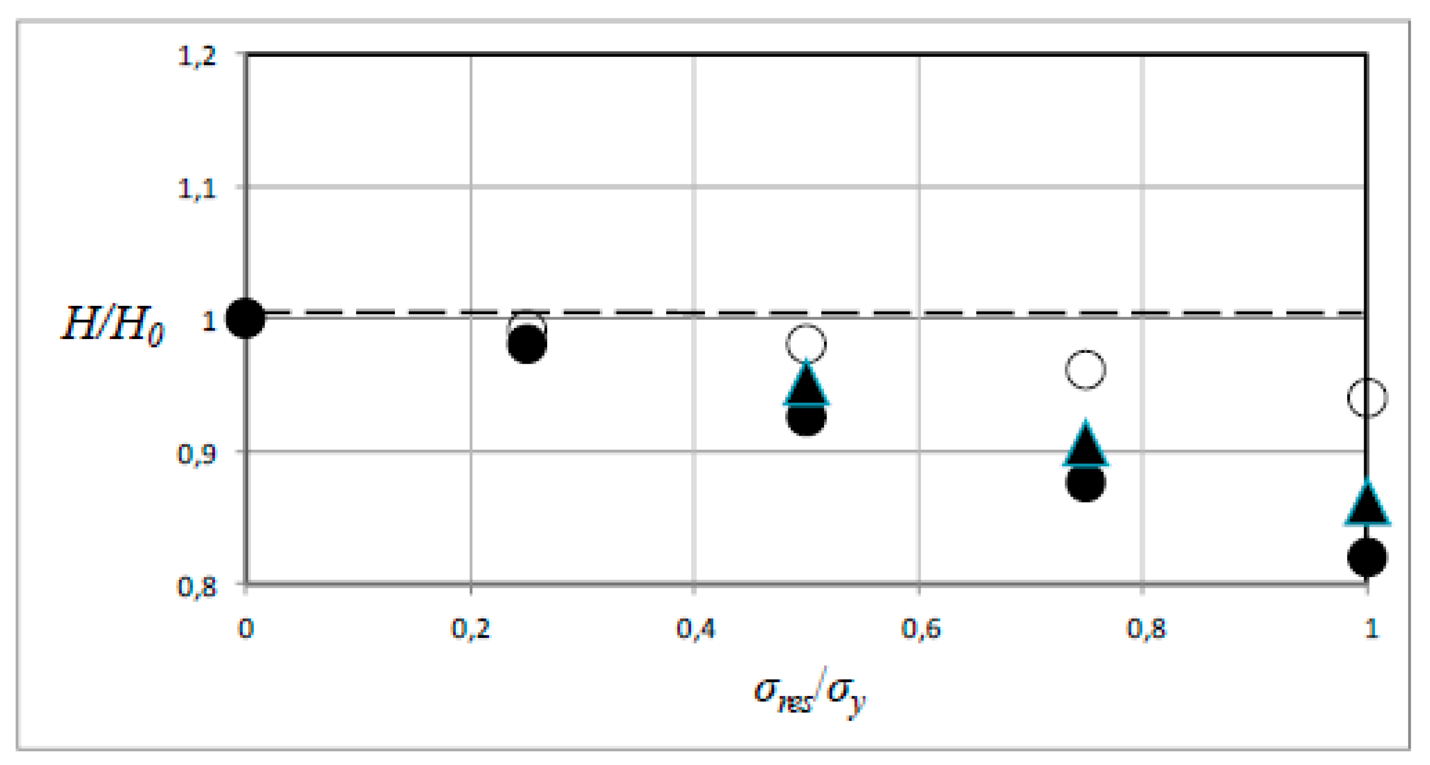
σres) for both these residual stress systems (obviously, this refers to a situation prior to indentation). The explicit results are shown in
Figure 5 where the non-dimensional hardness is depicted as function of the stress ratio (
σres/σy). Note that in
Figure 5 and below,
H0 is the hardness for the residual stress-free case. It is very clear from what is shown in
Figure 5 that the hardness is far more influenced by an equi-biaxial residual stress
σres than a corresponding uniaxial one. For example, at (
σres/σy) = 1, the hardness value is reduced (compared to the stress-free hardness
H0) with around 18% in the equi-biaxial case but with only approximately 6% in the uniaxial one. In practice, it would be very hard, if not experimentally impossible, to accurately determine
σres based on the small variation, in the uniaxial case, from the stress-free results.
Below are the results pertinent to residual surface stress states that depart from the strictly uniaxial and equi-biaxial. The reason for this is that equi-biaxial, but not uniaxial, stress states are experimentally determinable in a practical situation. It is then of interest to determine at what combination of principal residual stresses indentation experiments is a realistic alternative. In doing so, results for the particular case are:
which are in between the two extreme cases discussed above. In this context, it should be mentioned that based on Equation (11) then,
The results pertinent to Equations (11) and (12) are now presented in
Figure 6, together with the results shown in
Figure 5. Specifically, the cases
σres =
σy and
σres =
σy/2 are investigated.
As can be seen in
Figure 6, the new results fall essentially between the results for uniaxial and equi-biaxial stress states. In particular, it can be seen that the results for the stress state in Equations (11) and (12) indicate that experimental determination is practically achievable also in this case. This is indeed encouraging and deserves to be investigated further.
The hardness sensitivity (to residual stresses) is evaluated also for other values on the ratio:
The numerically derived results are shown
Figure 7 for the case
σ1 =
σres =
σy. It can be seen that at
k = 0.25, the influence from residual stresses on the hardness value is small and it seems appropriate to conclude that
k = 0.5 constitutes an approximate lower bound for the practical applicability of the present approach. For
k-values smaller than 0.5, the influence from residual stresses is so small that it would be difficult to measure any relevant changes of the material hardness in an accurate manner.
The corresponding results for the case σ
1 =
σres =
σy/2 are shown in
Figure 8. As could be expected, the practical applicability of the present approach is then very doubtful. Indeed, it can be argued that only in the case of equi-biaxial stresses any degree of accuracy of results can be expected.
It should be emphasized that the results above are only valid for the
Λ-value specified in Equation (10) (ln
Λ = 3.4). Correlation of the hardness variation with ln
Λ has been attempted previously [
13,
14] and as stated above, this correlation is acceptably accurate for equi-biaxial stresses but not so for uniaxial ones. As this state of affairs is in direct agreement with the results presented in
Figure 6,
Figure 7 and
Figure 8, correlation and accuracy deteriorate with decreasing values on
k; this feature will not be dwelled upon further.
Instead, the
Λ-dependence will be illustrated for a specific case, namely ln
Λ = 5.7. This is done in
Figure 9, where selected results for uniaxial and equi-biaxial stresses are presented. From what could be expected from the initial discussion in this subchapter, the
Λ-dependence is essentially non-existent (within the numerical accuracy) also at very high values on residual stresses (in the order of the material yield stress). It should be emphasized though that for values on ln
Λ smaller than 3.4, the hardness variation will be more pronounced in particular when it comes to range of values on
k.
Further, values on
Λ corresponding to rigid plastic contact, such as ln
Λ = 5.7, residual stress determination by indentation has to rely on the relative contact area
c2 in Equation (4). Corresponding results for equi-biaxial stresses, to the hardness results in
Figure 9, for this quantity for ln
Λ = 5.7, are shown in
Figure 10. Clearly, the
Λ-dependence is strong, which is encouraging. Such dependence has been shown previously [
3,
4,
5,
6,
7,
8], but here it is directly compared with the corresponding situation for the material hardness and established for a particular value on
Λ.
The nature of different types of residual stresses is of course a matter of basic importance for the present work. For one thing, when it comes to equi-biaxial residual stresses, such a situation can result from temperature loading of thin films or coatings on thick substrates. For more involved cases, for example residual stresses in bearings, gears, and cam-followers (with among other things implications for the onset of fatigue), studies presented in [
24,
25,
26] are referred to.
As a final comment, it should be emphasized that the present results are also of interest for other types of contact problems, i.e., the concerns of scratching and scratch testing where correlation using the Johnson [
15,
16] parameter
Λ also is a major issue, cf. [
27,
28,
29,
30].


