On the Two-Scale Modelling of Elastohydrodynamic Lubrication in Tilted-Pad Bearings

Abstract

A two-scale method for modelling the Elastohydrodynamic Lubrication (EHL) of tilted-pad bearings is derived and a range of solutions are presented. The method is developed from previous publications and is based on the Heterogeneous Multiscale Methods (HMM). It facilitates, by means of homogenization, incorporating the effects of surface topography in the analysis of tilted-pad bearings. New to this article is the investigation of three-dimensional bearings, including the effects of both ideal and real surface topographies, micro-cavitation, and the metamodeling procedure used in coupling the problem scales. Solutions for smooth bearing surfaces, and under pure hydrodynamic operating conditions, obtained with the present two-scale EHL model, demonstrate equivalence to those obtained from well-established homogenization methods. Solutions obtained for elastohydrodynamic operating conditions, show a dependency of the solution to the pad thickness and load capacity of the bearing. More precisely, the response for the real surface topography was found to be stiffer in comparison to the ideal. Micro-scale results demonstrate periodicity of the flow and surface topography and this is consistent with the requirements of the HMM. The means of selecting micro-scale simulations based on intermediate macro-scale solutions, in the metamodeling approach, was developed for larger dimensionality and subsequent calibration. An analysis of the present metamodeling approach indicates improved performance in comparison to previous studies.

1. Introduction

Tilted-pad bearings are found in lubricated rotating devices as they provide separation under heavy loads while keeping the power losses at a minimum [1]. It is the hydrodynamic action that generates pressure in the lubricant and gives the lifting force, and the bearing is said to operate under hydrodynamic lubrication (HL) conditions, if the pressure is not large enough to deform the bounding surfaces. Titled-pad bearings typically have a facing comprised of a compliant material, e.g., Babbitt and polytetrafluoroethylene (PTFE). This means that they operate under elastohydrodynamic lubrication (EHL) conditions where the pressure that is generated in the lubricant deforms the facing and sometimes also the backing, and significant fluid-structure interaction (FSI) occurs. The modelling approach including elastohydrodynamically generated FSI, is also well-established in the literature under the assumption of perfectly smooth surfaces [2,3,4]. For this purpose, it is conventional to use the Reynolds equation to model the hydrodynamic pressure generation, and to use infinitesimal strain theory to describe the deformation caused by the lubricant pressure. However, in lubricated contacts, surface micro-scale features, e.g., surface roughness, cannot be neglected as it contributes to the tribology at the interface. This also becomes more and more pronounced as the thickness of the film, separating the contacting bodies, becomes smaller and smaller. For example, Etsion [5] indicated that surface texturing can lead to a reduction of friction in EHL contacts and Greenwood and Johnson [6] showed that surface waviness generates ripples in the resulting pressure distributions. Other authors have developed deterministic models which aim to incorporate roughness into the simulations of EHL by modelling the features together with the bearing domain, see an example Reference [7,8,9,10,11,12]. These methods encounter significant computational limitations, due to requirements on grid density associated with the separation of scales between roughness and the contact region. Therefore, no general approach is yet accepted and authors have developed other approaches to modelling surface features in EHL, see e.g., the recent review paper by Vakis et al. [13].

One such approach is homogenization, in which information pertaining to a set of individual micro-scale surface features are characterized over a range of variables and subsequently coupled into a model for the macro-scale flow of the lubricant. Periodicity in the lubricant flow and surface features ensures that the homogenization process produces results representative of the mechanics at both scales. Stochastic theories such as those reported by Tzeng and Saibel [14] and by Christensen [15] are early ways of dealing with the effects of roughness by means of this type of two-scale approach in hydrodynamic lubrication. In his work Reference [16], Elrod was very early to present a homogenized Reynolds type of equation, obtained by multiple-scale analysis. Patir and Cheng [17,18] are precursors of an approach where the terms of the Reynolds equation are multiplied by flow factors to incorporate the effect of the surface features in the bearing fluid flow. The development of homogenization methods for HL has been investigated for a range of applications including compressible flows [19], mixed/boundary lubrication [20,21], tilted-pad bearings [22], porous media [23], inertial effects [24,25], cavitation [26] and soft contacts [27,28]. The rigorous mathematical derivation of these homogenization approaches is significantly different to that of Patir and Cheng [17,18] but exhibit similar responses under certain conditions [29]. Homogenization methods are preferable because they are capable of accurately describing the micro-scale effects in a macro-scale model without the associated computational requirements of deterministic modelling [30]. The requirement to include surface deformation, cavitation and other tribological phenomena has led to the derivation of more complex homogenization-based methods; see e.g., Reference [31,32,33].

One set of homogenization methods applicable to EHL are the Heterogeneous Multiscale Methods (HMM) [34,35], which describe a set of general techniques that facilitate a problem to be solved over multiple scales. The approach is applicable where there is at least an order of magnitude difference between these scales, as is the case when considering the bearing contact region and surface features. Gao and Hewson [36] were the first to derive the HMM in application to EHL and solved the influence of surface topography in sliding line contacts. In Reference [37], de Boer et al., subsequently generalized this two-scale method and adapted the approach for lubricant rheology, non-Newtonian behavior and inertial fluid flow. Part of the two-scale method is the use of metamodeling as a means of coupling the problem scales; this was investigated to allow surface features to be optimized for a minimum coefficient of friction [38]. Further studies based on the two-scale method have investigated line contact geometries [39] and cavitation at the scale of topography [40]. The HMM has also been applied to lubricated contacts by Pérez-Ràfols et al. [41] to investigate stochastic roughness in pressure-driven flows and metal-to-metal seals.

Hydrodynamic cavitation occurs in lubricated contacts when the pressure drops below the ambient value, causing air trapped in the lubricant to vaporize and form bubbles [1]. Conventionally, this does not occur in tilted-pad bearings where the fully-convergent shape of the film thickness prohibits such pressure being obtained. However, where there are divergent features, such as between the roller and the raceways in rolling element bearings or at the scale of surface topography, cavitation will be onset and must therefore be considered in such flows. Modelling of cavitation has been dominated by the well-established Elrod model [42] but the implementation and accuracy of such Heaviside methods are limited and authors have sought alternatives. More recently, the concept of complementarity has been applied to facilitate a more representative transition between the liquid and vapor phases in the contact, see e.g., Reference [43,44].

In connection to this, Pérez-Ràfols et al. [45] presented a very elegant transformation between incompressible and arbitrarily compressible pressure driven flow. de Boer and Dowson [46] recently solved the cavitation problem based on a moving mesh type approach, although film reformation was not implemented. Gao et al. [40] used hyperbolic tangents to reduce the fluid viscosity and density to capture the change in phases over a surface feature and explore micro-cavitation. This concept was more robustly explored by Söderfjäll et al. [47], who solved flows with textured surface features in oil control rings and introduced a model capable of describing the transition in phases accurately. The cavitation model of Söderfjäll et al. [47] is implemented in this article as a means of capturing the effects of micro-scale cavitation.

This article develops the two-scale method to EHL based on the HMM [36,37,38,39,40] to explore three-dimensional tilted-pad bearings. This includes modelling cavitation at the scale of the surface features and investigating the difference between ideal and real surface topographies on the solutions generated. The two-scale method is compared to the well-established homogenization methods [22] under HL conditions showing identical results. Subsequently the choice of the EHL model is analyzed in which the effects of material thickness and load capacity are explored. Two different surface topographies are investigated which facilitate ideal sinusoidal surfaces and real experimentally measured surfaces are directly compared. This showed that real surface topography has a stiffer response than in the ideal case. Simulations at the scale of topography indicated how periodicity was maintained and the effect of cavitation in the resulting distributions. Additionally, an analysis of the metamodeling approach used in coupling the problem scales is undertaken showing how the solution evolves and is calibrated throughout the solution procedure.

2. Materials and Methods

In this section the theoretical formulation for the two-scale method for modelling surface topography in tilted-pad bearings is outlined. Descriptions of both the macro and micro-scale models are given along with details for the metamodeling approach used to couple the scales and the corresponding solution procedure.

2.1. Macro-Scale Model

The macro-scale model considers the EHL of a three-dimensional tilted-pad bearing in which pressure generated in the lubricant causes deformation of the contacting surfaces, this interaction is fully-coupled to reach a specified load-carrying-capacity. The macro-scale geometry is depicted in Figure 1, showing an axially-symmetric (periodic) section of the bearing and the collar. The inner radius is $R_1$ and the outer radius is $R_2$, the bearing facing has a sector angle of ${\vartheta }_p$ and the sector angle of the periodic section ${\vartheta }_b$. The collar rotates with the angular velocity $\omega$ about the $z$-axis and lubricant, assumed to perfectly stick to the collar’s surface, is dragged into the divergent gap between the collar and the inclined bearing facing surface. At the macro-scale a fully separating fluid film is considered, thus assuming that there is no asperity contact nor any starvation at the interface. Additionally, the surface of the rotating collar is modelled as perfectly smooth and the bearing facing surface includes topography. Isothermal conditions are also applied.

Both the bearing backing and the collar has a thickness of $t_b$, and modeled, as they were made of stainless steel, with material data that is listed in

Table 1. Geometry and operating conditions of the macro-scale model.

Parameter	Value	Unit
$E_{PTFE}$	0.5	GPa
$E_{steel}$	200	GPa
$H_1$	2.5	μm
$L$	10, 30	N
$k$	10	MPa/μm
$R_1$	10	mm
$R_2$	20	mm
$t_b$	10	mm
$t_p$	0.1–10	mm
$t_0$	1	s
${\eta }_0$	0.3	Pa·s
${\vartheta }_b$	$2\pi /3$	rad
${\vartheta }_p$	$\pi /6$	rad
${\nu }_{PTFE}$	0.4	—
${\nu }_{steel}$	0.3	—
$\xi$	1	μm/(N·s)
${\rho }_0$	850	kg/m3
$\omega$	$500\pi /30$	rad/s

. The bearing pad facing is comprised of PTFE.

2.1.1. Solid Mechanics

A linear elastic model based on infinitesimal strain theory is used to consider solid deformation of the contacting surfaces in the macro-scale model. The governing equations are described in Equations (1)–(3) assuming steady-state conditions,

$$\nabla ·\mathit{\sigma }=0$$

(1)

$$\mathit{\sigma }=2\mu \epsilon +\lambda \mathrm{tr}\left(\mathit{\epsilon }\right)\mathit{I}$$

(2)

$$\mathit{\epsilon }=\frac{1}{2}\left[\nabla \mathit{u}+{\left(\nabla \mathit{u}\right)}^T\right]$$

(3)

where $\nabla =\left(\frac{\partial }{\partial X},\frac{\partial }{\partial Y},\frac{\partial }{\partial Z}\right)$ is the gradient operator for the $X,Y,Z$ Cartesian coordinate directions, $\mathit{I}$ is the identity matrix, $\mathit{u}=\left(u,v,w\right)$ is the vector of deformation components, $\mathit{\epsilon }$ is the strain tensor and $\mathit{\sigma }$ is the stress tensor. The shear modulus $\mu =E/2\left(1+\nu \right)$ and Lamé’s first parameter $\lambda =E\nu /\left(1+\nu \right)\left(1-2\nu \right)$ are related to the solid material Young’s modulus $E$ and Poisson ratio $\nu$ as indicated, these must be specified for the different materials in the model.

Two different cases are considered: (i) One which models the pad and collar simultaneously; and (ii) another which only considers the pad. The latter case is preferred since the computational requirements to model the simple geometry outweigh the benefits of including the collar in the simulation under certain conditions, as demonstrated by an example later in the article.

For Case (i), the boundary conditions are specified as follows. The lower surface of the collar backing is fixed such that deformation is zero $\mathit{u}=0$. The upper surface of the pad is loaded with load-per-unit-area $P^{*}$ such that $\mathit{\sigma }·\mathit{n}=-P^{*}\mathit{n}$, where $\mathit{n}$ is the surface normal vector. The boundaries of the collar representing axial-symmetry of the domain are coupled with a periodic condition such that their deformations are identical ${\mathit{u}}_{sym}$. All remaining boundaries are free to deform. It is of note that the load-per-unit-are $P^{*}$ relates to the lubricating pressure $P$ applied to the pad surface, see Section 2.1.4. A visualization of these boundary conditions is presented in Figure 2a. In Case (ii), the lower surface of the pad is specified using a fixed constraint $\mathit{u}=0$ and the remaining boundary conditions are the same as Case (i), see Figure 2b. This assumes that in Case (i) the magnitude of deformation of this surface is negligible in comparison to that of the upper surface of the pad, thus allowing the collar backing to be removed from the model.

2.1.2. Fluid Mechanics.

The macro-scale fluid flow considers conservation of mass and momentum and we adopt the Reynolds equation as the governing equation for lubricant transport in the thin film formed between the contacting surfaces. Flow factors are included in the formulation and describe the effect of homogenized surface topography in the macro-scale solution, as described in Section 2.3. The macro-scale fluid flow model to solve for the lubricating pressure $P$ is given by Equations (4)–(6),

$$Q_X=-{\psi }_{1,X}\frac{{\rho }_0{H}_m^3}{12{\eta }_0}\frac{\partial P}{\partial X}+{\psi }_{2,X}\frac{{\rho }_{0}U{H}_m}{2}$$

(4)

$$Q_Y=-{\psi }_{1,Y}\frac{{\rho }_0{H}_m^3}{12{\eta }_0}\frac{\partial P}{\partial Y}+{\psi }_{2,Y}\frac{{\rho }_{0}V{H}_m}{2}$$

(5)

$$\frac{\partial Q_X}{\partial X}+\frac{\partial Q_Y}{\partial Y}=0$$

(6)

where $Q_X$ and $Q_Y$ are the coordinate direction mass fluxes in the lubricating region, $H_m$ is the film thickness, ${\rho }_0$ is the macro-scale fluid density, ${\eta }_0$ is the macro-scale fluid viscosity, $U$ and $V$ are the components of rotational speed, and ${\psi }_{1,X},{\psi }_{2,X},{\psi }_{1,Y}$ and ${\psi }_{2,Y}$ are flow factors.

Incompressible and isoviscous conditions are considered such that the lubricant density and viscosity are constant in the macro-scale model. The rotational speed components are specified by defining a cylindrical coordinate system at the origin with the vertical component aligned to that of the Cartesian system: $r=\sqrt{X^2+Y^2}$; $\phi ={\tan }^{-1}\left(Y/X\right)$. Given an angular velocity of $\omega$ about the vertical axis of rotation yields $U=\omega r\cos \left(\phi \right)$ and $V=-\omega r\sin \left(\phi \right)$. Boundary conditions for the fluid flow problem are required on the outer perimeter of the upper surface of the pad, at each location the pressure is specified as that of the atmosphere $P=0$ (zero gauge).

2.1.3. Film Thickness

The macro-scale film thickness $H_m$ is given by the sum of the contact separation $H_0$, the pad geometry $H_g$, and the normal mechanical deformation of the pad surface $w_p=-\left(\mathit{u}·\mathit{n}\right)$. See Equation (7),

$$H_m=H_0+H_g+w_p.$$

(7)

where in this paper $H_g$ is described by Equation (8),

$$H_g=H_1\frac{r}{R_2}\frac{\sin \left(\phi \right)-\sin \left({\vartheta }_p/2\right)}{\sin \left(-{\vartheta }_p/2\right)-\sin \left({\vartheta }_p/2\right)}$$

(8)

with $H_1$ being the pad differential film thickness. Subsequently, Equation (9) provides a relation between $H_m$ and $H$ which is the film thickness used to couple scales of the problem,

$$H=H_m-\delta$$

(9)

where the local deformation of the pad is $\delta$. This local deformation is modelled at the micro-scale, see Section 2.2.

2.1.4. Load-Per-Unit-Area

The load-per-unit-area $P^{*}$ and the pressure $P$ differ because of the multiscale approach, see Section 2.2. At the macro-scale, $P^{*}$ is used to determine deformation and load capacity, whereas $P$ is the solution to the macro-scale fluid flow problem Equations (4)–(6). An additional relation is made between these two variables by introducing a further flow factor ${\psi }_p$, see Equation (10).

$$P^{*}={\psi }_{p}P$$

(10)

In the case where all flow factors are identical to unity, e.g., $\psi \equiv 1$, the problem reduces to the perfectly smooth problem. However, when the flow factors deviate from unity, the solution incorporates the effect of topography in the macro-scale model. The flow factors are functions of 6 macro-scale variables, which couple the macro with the micro-scale, namely the pressure $P$; the pressure gradients $\frac{\partial P}{\partial X}$ and $\frac{\partial P}{\partial Y}$; the film thickness $H$; and the surface velocities $U$ and $V$. In other words, $\psi =\psi \left(P,\frac{\partial P}{\partial X},\frac{\partial P}{\partial Y},H,U,V\right)$ and the reader is referred to Section 2.3 for the details on how the flow factors are determined.

2.1.5. Load Carrying Capacity

The load carrying capacity of the contact is also modelled at the macro-scale. The requirement is that the bearing should hold a specified load $L$ (given as an input) as described by Equation (11),

$$L=\iint P^{*}dS$$

(11)

where $S$ is the surface area of the pad. To achieve this force-balance requirement, the contact separation $H_0$ is considered as a dependent variable, which takes a unique value given a specified load large enough not to collapse the film completely. A monotonic increase in $L$ leads to a monotonic decrease in $H_0$, and vice versa, and this relation is the basis for a quasi-static solution procedure to achieve the required load. The procedure is outlined in Section 2.4.

2.2. Micro-Scale Model

The micro-scale model considers the EHL of a domain independent of the tilted-pad bearing, in which a homogenized pressure $P$, pressure gradients $\frac{\partial P}{\partial X}$ and $\frac{\partial P}{\partial Y}$, film thickness $H$ and surface velocities $U$ and $V$ defined at the macro-scale determine the micro-scale parameters. The model is based on the HMM [32,33] and is valid so long as two assumptions are upheld: (i) the size of the micro-scale domain is an order of magnitude, or more less than that of the macro-scale domain; and (ii) periodicity in geometry and flow conditions are maintained in the micro-scale.

The geometry is specified by considering two length scales $l_x$ and $l_y$ that describe the bounds of the micro-scale domain ${\Omega }_{\mu }=\left\{0\le x\le l_x,0\le y\le l_y\right\}$, where $x$ and $y$ are the micro-scale Cartesian coordinate directions. The value of each is chosen based on a wavelength $\epsilon$ relative to the size of the macro-scale model $l_x,l_y=\epsilon \left(l_X,l_Y\right)$, where $l_X,l_Y=R_2-R_1$ quantify the largest length scale of the macro-scale domain in each of the coordinate directions. The wavelength must be selected such that there is at least an order of magnitude difference between the macro and micro length scales, e.g., $\epsilon <{10}^{-1}$. This assumption limits the size of surface topographies which can be investigated using the two-scale approach. However, the assumption of $\epsilon <{10}^{-1}$ is consistent with the scaling used in deriving the Reynolds equation. Conversely, as the wavelength increases the assumption of near parallel surfaces in contact becomes further from that represented by the two-scale mechanics, the model breaks down. Given periodicity in the geometry and fluid flow as the wavelength tends to zero the solution to the micro-scale problem becomes that described exactly by the Reynolds equation.

It is possible to include phenomena in the micro-scale model which are not described by the macro-scale mechanics alone, in this formulation we are concerned with surface topography and the resulting effects of cavitation.

2.2.1. Fluid Mechanics

Micro-scale fluid flow is modelled by considering the conservation of mass and momentum in the lubricant according to the Reynolds equation. Mathematically, the fluid transport at the micro-scale domain ${\Omega }_{\mu }$ is described by Equations (12)–(14),

$$q_x=-\frac{\rho h^3}{12\eta }\frac{\partial p}{\partial x}+\frac{\rho Uh}{2}$$

(12)

$$q_y=-\frac{\rho h^3}{12\eta }\frac{\partial p}{\partial y}+\frac{\rho Vh}{2}$$

(13)

$$\frac{\partial q_x}{\partial x}+\frac{\partial q_y}{\partial y}=0$$

(14)

where $q_x$ and $q_y$ are the micro-scale mass flux (per unit depth) in each coordinate direction, $p$ is the micro-scale pressure, $h$ is the micro-scale film thickness, $\rho$ is the micro-scale fluid density, and $\eta$ is the micro-scale fluid viscosity.

The solution to Equations (12)–(14) are achieved by specifying periodic boundary conditions for the pressure at the extents of the micro-scale domain $p\left(l_x,y\right)=p\left(0,y\right)+{\Delta }_{x}p$, $p\left(x,l_y\right)=p\left(x,0\right)+{\Delta }_{y}p$, where ${\Delta }_{x}p$ and ${\Delta }_{y}p$ are the micro-scale pressure differences in each of the coordinate directions. These conditions are imposed such that the distribution of pressure on each set of boundaries are the same, but their magnitudes differ by a constant value, as defined by the macro-scale pressure gradients ${\Delta }_{x}p=l_x\frac{\partial P}{\partial X},{\Delta }_{y}p=l_y\frac{\partial P}{\partial Y}$.

In combination with the periodic boundary conditions, a pressure point constraint must be included to solve the problem. This is defined by two requirements: (i) the average pressure in the micro-scale domain should represent the macro-scale pressure; and (ii) there should be no pressure defined on the boundary which is negative, due to the requirements of cavitation. To satisfy the first requirement, a constraint pressure $p_0$ is specified according to Equation (15),

$$p_0=P+\frac{1}{2}\mathrm{sgn}\left(-{\Delta }_{x}p\right)\left|{\Delta }_{x}p\right|+\frac{1}{2}\mathrm{sgn}\left(-{\Delta }_{y}p\right)\left|{\Delta }_{y}p\right|$$

(15)

which is ideally imposed at the origin of the micro-scale domain. If this condition is upheld and it results in a negative pressure on any of the boundaries, a solution will then not be physically representative when cavitation is considered, see Section 2.2.2. Therefore, a minimum required pressure is calculated $p_m=\min \left(p_0,p_0+{\Delta }_{x}p,p_0+{\Delta }_{y}p,p_0+{\Delta }_{x}p+{\Delta }_{y}p\right)$ and the pressure point constraint is given by Equation (16).

$$p\left(0,0\right)=\{\begin{array}{cc}{p}_0\hfill & \hfill p_m\ge 0\\ p_0-p_m\hfill & \hfill p_m<0\end{array}$$

(16)

2.2.2. Cavitation

Cavitation is considered in the micro-scale model because, unlike the macro-scale model where the shape of the contact is fully convergent, the micro-scale geometry will have converging-diverging geometrical features relating to surface topography. Therefore, under low pressure conditions, cavitation will occur in the diverging regions, and if left unmanaged, will produce non-physical negative pressures. It is a conventional to approach the cavitation problem by rapidly reducing the fluid density and viscosity as the pressure drops below a zero gauge to represent a transition from liquid to vapor phases. In this article, Söderfjäll’s et al. [47] cavitation model is adopted as described by Equation (17),

$$f=\{\begin{array}{cc}1\hfill & p>0\\ 1-2{\left(\frac{p}{\beta }\right)}^3-3{\left(\frac{p}{\beta }\right)}^2\hfill & -\beta \le p\le 0\\ 0\hfill & p<-\beta \end{array}$$

(17)

where $f$ is the degree of saturation of the fluid and $\beta$ is a threshold pressure. The micro-scale fluid density and viscosity are subsequently expressed by Equations (18) and (19), respectively, where $\alpha$ is threshold constant and takes a value approaching zero. The values of $\alpha$ and $\beta$ used in this study are the same as Söderfjäll’s et al. [47] and are given in

Table 2. Parameters used in defining surface topography at the micro-scale.

Parameter	Value	Unit
$A$	1	μm
$\alpha$	0.01	—
$\beta$	0.2	MPa
$\epsilon$	2−4, 2−5	—

.

$$\rho ={\rho }_0\frac{f+\alpha }{1+\alpha }$$

(18)

$$\eta ={\eta }_0\frac{f+\alpha }{1+\alpha }$$

(19)

2.2.3. Film Thickness

The micro-scale film thickness is described by Equation (20),

$$h=H+h_t+\delta$$

(20)

where $h_t$ is a function defining the surface topography and $\delta$ is the micro-scale deformation. This deformation is equal to that of a spring with stiffness-per-unit-area $k$ under a load-per-unit-area of $P^{*}$, see Equation (21).

$$\delta =\frac{P^{*}}{k}$$

(21)

The function describing topography must be periodic on the micro-scale boundaries $h_t\left(l_x,y\right)=h_t\left(0,y\right)$, $h_t\left(x,l_y\right)=h_t\left(x,0\right)$ but can take any value within the domain. Additionally, $h_t$ must have an average value over the domain of zero such that the average initial film thickness (without deformation) is equal the macro-scale film thickness $H$. The load-per-unit-area is subsequently determined from the average micro-scale pressure, as given by Equation (22),

$$P^{*}\left(P,\frac{\partial P}{\partial X},\frac{\partial P}{\partial Y},H,U,V\right)=\frac{1}{l_x{l}_y}\iint pdxdy$$

(22)

and is a function of the 6 variables used to couple the problem scales. The pressure $P$ and load-per-unit-area $P^{*}$ differ because, at the micro-scale pressure, it is not uniformly distributed over the domain due to the presence of topography and cavitation; as such, there are different contributions made in coupling the fluid flow and solid deformation in the two-scale model. In the model derived here, the micro-scale deformation is a constant value over the domain, to include deformation as a function of the micro-scale domain, an equivalent solid thickness can be derived from the material and stiffness properties of the problem, as previously investigated by the authors in Reference [38,40]. This effect has been neglected due to the large increase in computational costs, where only a 0.5% change in the micro-scale surface topography would be expected under the conditions imposed [38,40].

2.2.4. Homogenization

To couple the micro-scale data to the macro-scale information, it is homogenized and mapped across the scales. The homogenized variables become functions of the 6 parameters used in defining the micro-scale model, resulting in Equation (21) for $P^{*}$, and Equations (23)–(24),

$$Q_X\left(P,\frac{\partial P}{\partial X},\frac{\partial P}{\partial Y},H,U,V\right)=\frac{1}{l_y}\int q_x\left(0,y\right)dy$$

(23)

$$Q_Y\left(P,\frac{\partial P}{\partial X},\frac{\partial P}{\partial Y},H,U,V\right)=\frac{1}{l_x}\int q_y\left(x,0\right)dx$$

(24)

for $Q_X$ and $Q_Y$, respectively. The boundaries $\left[0,y\right]$ and $\left[x,0\right]$ are chosen to assess the integrals arbitrarily from $\left[l_x,y\right]$ and $\left[x,l_y\right]$. The variables $Q_X$, $Q_Y$ and $P^{*}$ are subsequently expressed at the macro-scale by the use of flow factors in Equations (4), (5) and (10). Therefore, the flow factors describe fluctuations in the mass flux and the load-per-unit-area at the macro-scale due to the inclusion of surface topography and cavitation in the micro-scale model.

2.3. Flow Factors

A metamodeling approach is used to calculate the flow factors that couple to the macro and micro-scale models. The Moving Least Squares (MLS) method is employed to derive a multidimensional metamodel of the macro-scale variables $\zeta =\left(P,\frac{\partial P}{\partial X},\frac{\partial P}{\partial Y},H,U,V\right)$ to determine each of the flow factors $\psi$. Underpinning the calculation of flow factors is the requirement for a range of predetermined micro-scale experiments to be known such that the metamodels can be assessed. This forms the metamodel building stage in which a Design of Experiments (DOE) is used to determine which micro-scale experiments to collect data for. As part of the metamodel building, a Cross Validation (CV) procedure is used to tune the metamodel fit to the known data. Since the macro-scale solution procedure is an iterative process (see Section 2.4), additional micro-scale data is required and the DOE evolves with solution time according to the instantaneous difference in macro-scale parameters. The procedure outlined develops the approach de Boer et al. [39] implemented for investigating highly loaded line contacts and aims to improve both accuracy and efficiency for higher dimensionality when using metamodels as a means of coupling the problem scales.

2.3.1. Moving Least Squares

In each of Equation (4), (5) and (10), the left-hand-side terms are written as a series summation of flow factors multiplied by terms that are only functions of the variables in $\zeta$. Subsequently, by using these equations as the basis functions, a regression analysis allows $\psi$ to be assessed as coefficients, given a known set of data from the DOE.

MLS is a form of conventional least squares regression in which the coefficients do not remain constant but instead become functions of the space in which the metamodel is assessed $\psi =\psi \left(\zeta \right)$. A weighting parameter γ is introduced to change the influence of known data points in the regression analysis. A Gaussian decay type function is conventionally used such that the weight diminishes with increasing Euclidian distance from the assessment location as described by Equation (25),

$${\gamma }_i\left(\zeta \right)=\exp \left(-\theta {ɍ}_i^2\right)i=1,\dots ,n$$

(25)

where $\theta$ is the closeness of fit and ${ɍ}_i^2$ is the square of the normalised Euclidian distance between the $i$’th known experiment and assessment location $\zeta$, and $n$ is the number of data points in the DOE. The normalised Euclidian distance is given by Equation (26),

$${ɍ}_i^2={\displaystyle \sum _{j=1}^{j=6}}{\left({\overline{\zeta }}_{i,j}-{\overline{\zeta }}_j\right)}^2$$

(26)

where ${\overline{\zeta }}_j$ is the normalised $j$’th component dimension of $\zeta$, and ${\overline{\zeta }}_{i,j}$ is the normalised $j$’th component dimensionof $\zeta$ for the $i$’th known experiment. The normalised variables of $\zeta$ are obtained from ${\overline{\zeta }}_{i,j},{\overline{\zeta }}_j=\left(\left({\zeta }_{i,j},{\zeta }_j\right)-\underset{i}{\min }\left({\zeta }_{i,j}\right)\right)/\left(\underset{i}{\max }\left({\zeta }_{i,j}\right)-\underset{i}{\min }\left({\zeta }_{i,j}\right)\right)$.

An example of the MLS metamodel building is presented in Equation (27) for the variable $Q_X$,

$$\left[\begin{array}{c}{\gamma }_1{Q}_{X,1}\\ ⋮\\ {\gamma }_n{Q}_{X,n}\end{array}\right]=\left[\begin{array}{cc}-{\gamma }_1\frac{{\rho }_0}{12{\eta }_0}{(H_1+\frac{P_1^{*}}{k})}^3{\left(\frac{\partial P}{\partial X}\right)}_1& {\gamma }_1\frac{{\rho }_0}{2}{U}_1(H_1+\frac{P_1^{*}}{k})\\ ⋮& ⋮\\ -{\gamma }_n\frac{{\rho }_0}{12{\eta }_0}{(H_n+\frac{P_n^{*}}{k})}^3{\left(\frac{\partial P}{\partial X}\right)}_n& {\gamma }_n\frac{{\rho }_0}{2}{U}_n(H_n+\frac{P_n^{*}}{k})\end{array}\right]\left[\begin{array}{c}{\psi }_{1,X}\\ {\psi }_{2,X}\end{array}\right]$$

(27)

where additional subscripts denote the position in the DOE. The metamodel is assessed numerically as a system of overdetermined equations to give the flow factors ${\psi }_{1,X}$ and ${\psi }_{2,X}$ as a function of the space described by $\zeta$, a matrix operation is required for each assessment location and there is no analytical form of the metamodel. This formulation is derived in a similar manner for the remaining metamodels, required as part of the two-scale method, $Q_Y$ and $P^{*}$.

2.3.2. Closeness of Fit

The closeness of fit $\theta$ controls the rate of decay of the MLS weighting functions and therefore provides a means of tuning the response of the metamodel to minimise the error between the predicted and known values. In the case where $\theta =0$ the weights become equal to unity and the MLS metamodel reduces to a conventional least squares regression, under these conditions the resulting coefficients are constant. In the opposing case where $\theta \to \infty$ the influence of all data points on the response becomes zero and the metamodel does not provide a measureable quantity.

A value of $\theta$ must be chosen for each of the metamodels required as part of the two-scale method, this is achieved by conducting CV studies on the known DOE data. In this process, a range of $\theta$ values are inspected and the one that produces the lowest absolute error between the known data points and that predicted by the metamodel is selected as the true value. After the true $\theta$ value is known the metamodel can be assessed to produce the flow factors as a function of the design variables.

The CV procedure implemented in this article is known as the Leave-One-Out method. In this method, a range of the closeness of fit parameters are selected. Subsequently, and for each value of $\vartheta$, all data points in the DOE are removed in turn and the metamodel built from the remaining DOE values. Then, the absolute error between the metamodel predication and the removed DOE value is assessed. By repeating and averaging all the DOE points, the mean error is given, and by varying $\theta$, the best value can be selected, that is, the one which minimises the mean error. This final value of $\theta$ is the one for which the metamodel is assessed to determine the flow factors.

2.3.3. Design of Experiments

The flow factors $\psi$ are calculated at the macro-scale from MLS metamodels of the homogenized micro-scale data and are updated as the solution procedure progresses, see Section 2.4. For each interim macro-scale solution, a check is performed on the DOE to determine whether additional micro-scale experiments are required. This check adds DOE data points based on whether the new solution is far from the previously known information, such that the flow factors will be accurately described in the current region of interest.

At any instance within the macro-scale solution procedure, the homogenized variables describe a curve within a 6-dimensional space, as defined by $\zeta =\left(P,\frac{\partial P}{\partial X},\frac{\partial P}{\partial Y},H,U,V\right)$. The curve is given from Equation (28),

$${\left(\partial s\right)}^2={\displaystyle \sum _{j=1}^{j=6}}{\left(\partial {\zeta }_j\right)}^2$$

(28)

where $s$ is the arc length of the curve $\zeta$. The curve is discretized by dividing it into 1000 evenly-spaced points along $s$. Then, based on the normalised Euclidian distance between the curve and the current DOE points, additional points are added to the DOE if they are more than 1% from it. In the case where no data points exist (first iteration of the macro-scale solution procedure), then the entire curve is added. For each of the added points, the corresponding micro-scale simulations are assessed and the MLS metamodels are updated. In the subsequent CV procedure, the range of the closeness of fit $\theta$ is chosen based on the current known value and increased/decreased by 50%, or in the case where no value (or a zero value) of $\theta$ has been determined, $0\le \theta \le 3000$ is implemented.

2.4. Macro-Scale Solution Procedure

Macro-scale solutions were calculated using the software Comsol Multiphysics [48] in which the domain and governing equations were discretized using the Finite Element (FE) method. In the first instance, solutions without topography were solved to provide initial estimates for the cases where topography was included. To do this, Equations (1)–(3) were solved in the solid phase and Equations (4)–(6) were solved in the fluid phase. The interaction was full-coupled through the boundary load applied to the pad surface and the flow factors were equal to unity $\psi =1$. Initially, an arbitrary value of $H_0=5$ μm was specified (this value was chosen to allow a comparison to the hydrodynamic case without deformation) and was subsequently changed to balance the required load capacity, according to Equation (29),

$$\frac{\partial H_0}{\partial t}=\xi \left(\iint P^{*}dS-L\right)$$

(29)

where $t$ is the solution time and $\xi$ is a positive constant. At each increment of $H_0$ in Equation (29), the initial solution to pressure became the solution of the previous time step, for the first time step, a zero initial solution was assumed. The total solution time $t_0$ is chosen arbitrarily and the magnitude of $\xi$ is changed to achieve numerical convergence over $0\le t\le t_0$. In the case without topography, the flow factors are each specified as $\psi =1$ over the entire macro-scale domain.

Referring to Section 2.1, Case (i), inclusive of the pad and collar together, were discretized using 65,000 2nd order tetrahedral elements in total. A sensitivity study of this mesh demonstrated a less than 1% improvement in predicting the maximum lubricating pressure when a greater number of elements were used. Similarly, for Case (ii) in which the pad was modelled alone, a mesh of 7800 2nd order tetrahedral elements were shown to give the same level of accuracy as Case (i). To allow the results produced to be compared to the literature, see Almqvist [22], a hydrodynamic case without deformation was considered. Case (iii) therefore modelled the pad surface alone in two-dimensions and there was no coupling to the solid, in this model the domain was discretized using 1200 2nd order triangular elements. Again, with no significant change in the maximum pressure calculated when using a more refined mesh. All computations were performed on an Intel Xeon CPU (Intel Corporation, Santa Clara, CA, USA) with 4 cores operating at 3.3 GHz.

2.4.1. Micro-Scale Effects

Micro-scale effects, as described by flow factors, were included in the macro-scale solution by using the results without topography as an initial solution. Based on the 6-dimensional curve describing this solution $\zeta =\left(P,\frac{\partial P}{\partial X},\frac{\partial P}{\partial Y},H,U,V\right)$, the DOE and corresponding micro-scale solutions were calculated and the metamodels built, see Section 2.5. Subsequently, the flow factors were calculated as functions of the initial macro-scale solution and kept constant throughout the remainder of the procedure. The macro-scale solver was then computed for the current flow factors and the new solution generated was checked for convergence in the maximum normalized pressure predicted. The criteria implemented measures the difference in maximum pressures measured between two iterations and divided by the maximum pressure of the previous iteration. If there was no convergence, the DOE check is conducted and additional micro-scale simulations conducted were required. When the size of the DOE was increased, the metamodel tuning parameters were updated by undertaking a further CV study. After the metamodel was updated, the initial solution and flow factors were updated based on the current solution and the process was repeated until convergence was reached. The calculation of flow factors and metamodel building was undertaken using Matlab [49]. All solver tolerances were set to 10⁻³ to ensure the accuracy of the returned solutions.

2.4.2. Macro-Scale Parameters

The geometry and operating conditions used to describe the macro-scale calculations undertaken in this article are given in Table 1. These have been chosen to provide meaningful comparisons to the work of Almqvist [22] who studied the homogenized influence of surface topography in hydrodynamic tilted-pad bearings.

2.5. Micro-Scale Solution Procedure

Micro-scale simulations were calculated by inheriting the parameterized variables from the macro-scale $P,\frac{\partial P}{\partial X},\frac{\partial P}{\partial Y},H,U$ and $V$ such that for any combination of them, a solution to $Q_X,Q_Y$ and $P^{*}$ can be obtained. Comsol Multiphyics [48] was used to solve Equations (12)–(14) for the fluid phase along with Equation (20) for the solid phase to provide the micro-scale solutions by the application of the FE method. The initial value for pressure in the micro-scale domain was specified according to Equation (29),

$$p=p\left(0,0\right)+{\Delta }_{x}p\frac{x}{l_x}+{\Delta }_{y}p\frac{y}{l_y}$$

(29)

which is consistent with the constraint pressure specified in Equation (16).

For the micro-scale domain, a mesh of 6000 2nd order triangular elements were used for all surface topographies and the cases were considered. This was found to produce grid independent results with a change of less than 1% in the maximum pressure observed when using a more refined domain. The same CPU, as described in Section 2.4, was used to calculate the micro-scale solutions; the solver tolerance was specified as 10⁻³ for convergence.

2.5.1. Surface Topography

Two definitions of surface topography are investigated in the remainder of this article: (i) an ideal topography; and (ii) a real topography. Each represents a periodically repeating surface feature over the macro-scale domain, changes in topography from one location to the next can be achieved at the macro-scale so long as the variation is continuous. However, this is beyond the scope of the current paper. The opposing boundary values of the surface topography function are identical and the length scales must be chosen so that they are consistent with the required scale separation of the HMM used in deriving the model.

The function used to describe the ideal surface topography is given by Equation (31),

$$h_t=\frac{A}{2}\cos \left(\frac{2\pi x}{l_x}\right)\cos \left(\frac{2\pi y}{l_y}\right)$$

(31)

where $A$ is the amplitude and $h_t$ is consistent with that implemented by Almqvist [22].

In the case of real topography, experimental data for a PTFE pad was measured using a vertical scanning interferometer. This provided height data for the real surface as a function of the Cartesian coordinate directions. Subsequently, the experimental data was processed by implementing a 2-dimensional Fourier transformation in Matlab [49], the resulting power spectrum was truncated to keep the top 10% of frequencies and the inverse transformed to create a smooth continuous function representing the real data. To provide a periodic function, the real surface data was mirrored about both the x and y-axes. Lastly, the mean value of the function over x and y was determined and taken away from the mirrored function to give $h_t$ for the experimental data, this facilitates that the micro-scale domain represents the macro-scale film thickness $H$ without deformation.

2.5.2. Micro-Scale Parameters

To define surface topography and the micro-scale model, additional parameters were introduced and values for these are given in Table 2. These have been selected to generate meaningful solutions, but also to directly compare with the results of Almqvist [22]. Note that the value of $\epsilon$ is selected such that the required separation of scales is maintained. The sizes of the micro-scale domain $l_x$ and $l_y$ are subsequently derived, for which the surface topography function $h_t$ is scaled accordingly.

3. Results

In this section results are presented for the two-scale model to demonstrate the following: (i) verification of the two-scale method in comparison to well-established homogenization methods under hydrodynamic conditions; (ii) verification of the choice of macro-scale EHL model comparing the pad and collar to the pad alone; (iii) macro-scale solutions with topography generated by the two-scale method; (iv) examples of micro-scale solutions corresponding to the macro-scale results; and (v) examples of the metamodel performance and verification for coupling the problem scales.

3.1. Verification of the Two-Scale Model under Hydrodynamic Conditions

A comparison of the results generated by the two-scale method under hydrodynamic conditions and the homogenization approach of Almqvist [22] was undertaken. For this purpose, simulations were calculated under the conditions described by Case (iii) in Section 2.4 without the load balance considered and $H_0=5$ μm. At the micro-scale, the ideal topography was used and cavitation was not modelled, this allowed a direct comparison between the two sets of results.

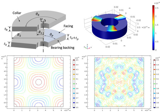
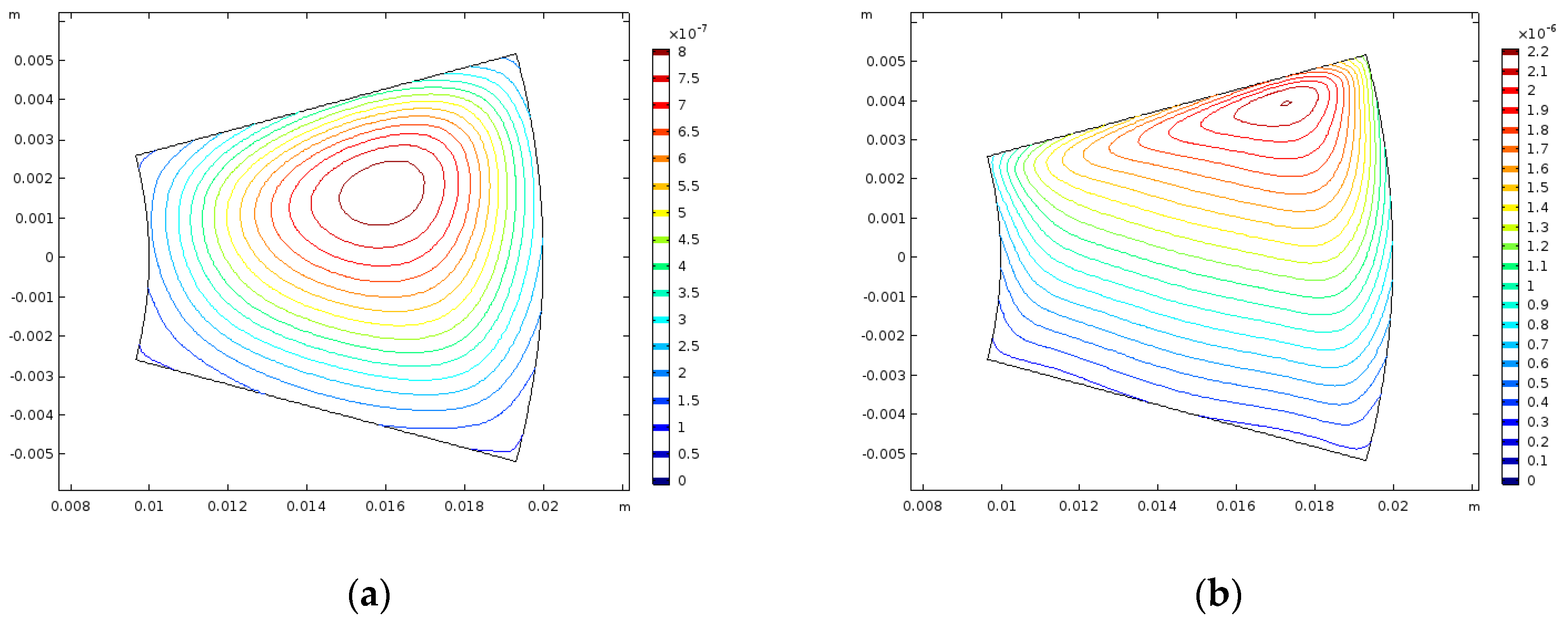
Figure 3a,b presents the macro-scale pressure distributions from the two-scale method resulting from this analysis, where two different scale separations are investigated. Both values of $\epsilon$ satisfy the requirements of the HMM in defining the two scales and are both presented for the same conditions by Almqvist [22]. The pressure distributions for the two scale separations are shown to be very close together in Figure 3a,b, with an 87 Pa difference being the maximum value between any two elements on the pad surface in the corresponding simulations. This result was expected since changing the size of the micro-scale domain under hydrodynamic conditions with no cavitation leads to a direct scaling of the homogenized variables. Additionally, a visual comparison between these results and those presented by Almqvist [22] shows that they are similar. This verifies the two-scale model against the well-established homogenization methods for lubricated contacts under hydrodynamic conditions and indicates the scope of the two-scale method for modelling EHL including the effects of surface topography.

3.2. Verification of the Choice of Macro-Scale EHL Model

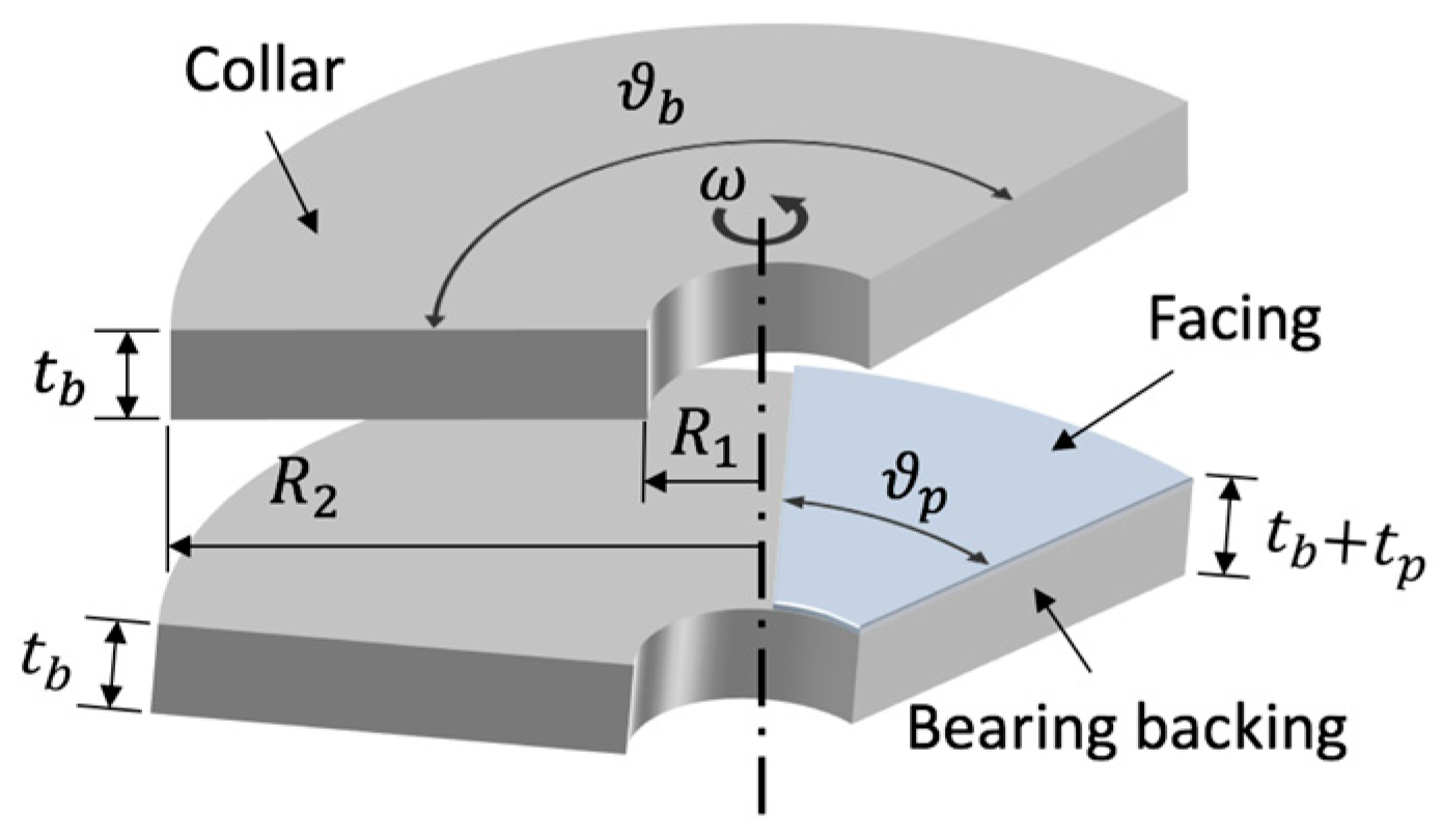
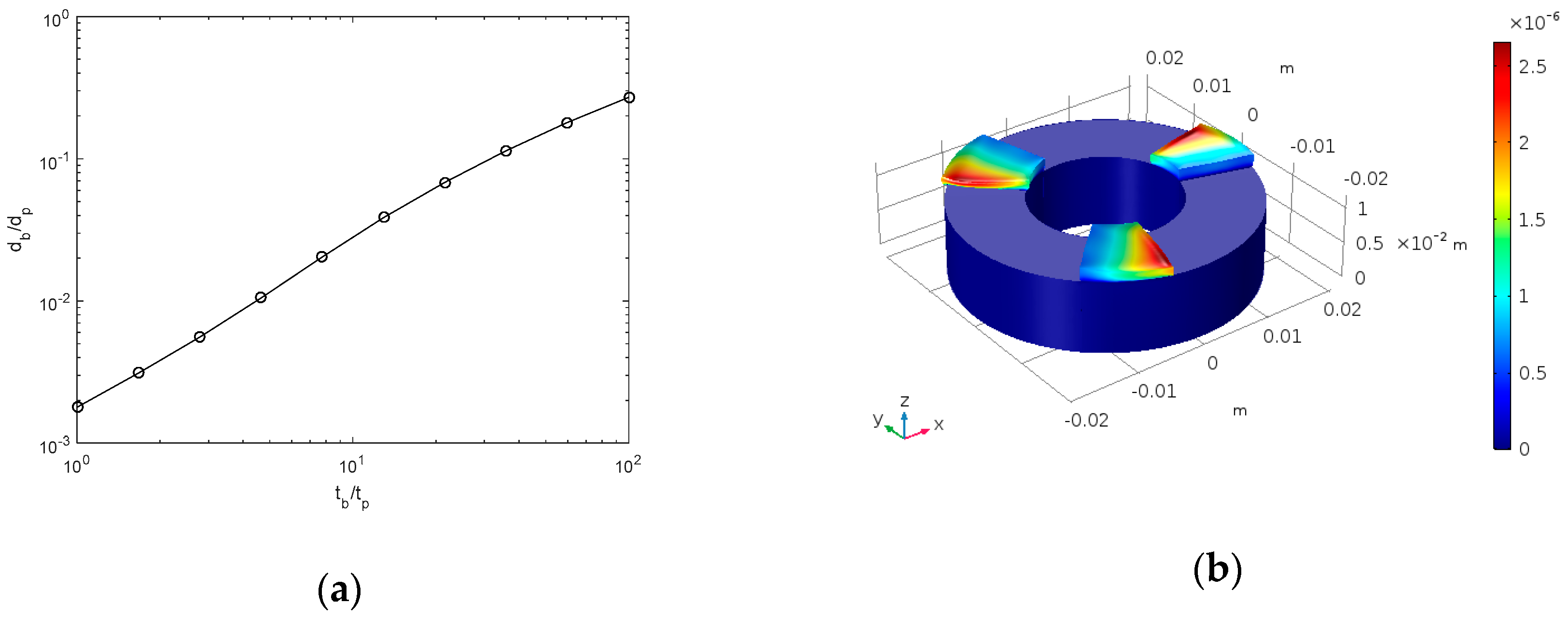
To establish the choice of macro-scale EHL models, a study into the effect of modelling the pad and backing together versus modelling the pad alone was undertaken. In this analysis, the thickness of the pad $t_p$ was varied between 0.1 mm and 10 mm with the backing thickness kept constant at $t_b=10$ mm. The contact separation was kept constant at $H_0=5$ μm and the load balance was not considered. A range of calculations were then conducted according to Case (i), and as described in Section 2.4, surface topography was not included in the model and as such all flow factors in the model were set to unity $\psi =1$. Average deformations were then calculated according to Equation (32),

$$d_b,d_p=\frac{2}{{\vartheta }_p\left(R_2^2-R_1^2\right)}\iint \left(w_b,w_p\right)dS$$

(32)

where $d_b$ is the average deformation of the backing, $d_p$ is the average deformation of the pad and $w_b$ is the surface deformation of the backing. The ratio of these deformations is plotted against the ratio of thicknesses and is presented in Figure 4a. As the pad decreases in thickness, the proportion of backing deformation increases in comparison to that of the pad itself, implying that as the pad becomes thinner, the requirement to model the collar becomes more important. Additionally, for a pad of thickness $t_p=2$ mm, and a backing thickness $t_b=10$ mm, the ratio of deformations is approximately 0.01, which can be considered small enough to neglect and assume that the backing deformation is negligible. This verifies the choice to model the pad under EHL conditions without including the backing, as described by Case (ii) in Section 2.4. This assumption is carried forward throughout the remainder of the results presented. A visualization of the deformations generated in pad and backing models, under these conditions, is presented in Figure 4b. The result has been mirrored in the axial line of symmetry to show the full bearing and the volume was deformed according to a scale factor of 500 with the deformation field exaggerated and visually observed in the solution.

A further consideration to make is that the choice of macro-scale EHL model is load dependent, with larger loads causing larger deformations of both the pad and collar, thus moving further from the assumption that the backing is fully constrained. Two further simulations were undertaken at the macro-scale using the pad and backing model (for the thicknesses described previously), neglecting surface topography but including the load balance. Two loads were chosen, $L=10$ N and $L=30$ N, to show the dependence of increasing the load on the resulting film thickness and deformation distributions. The results are presented in Figure 4a,b for these two loads, respectively, showing deformation of the pad surface. A measurement is introduced in Equation (33) to quantify the differences in the average trailing edge film thickness $H_{te}$,

$$H_{te}=\frac{1}{R_2-R_1}\int H_{m}dr$$

(33)

where the integration is performed on the boundary $\left[r,{\vartheta }_p/2\right]$, as defined in the polar coordinate system.

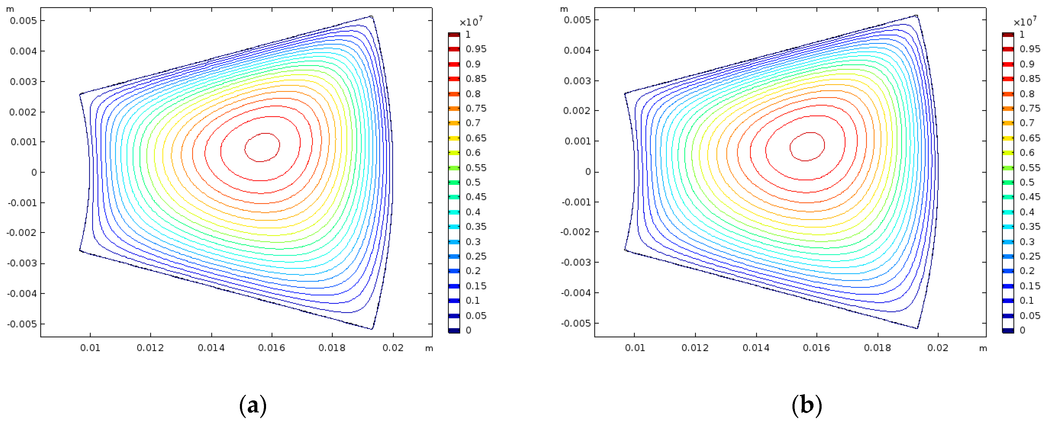
The low load result, depicted in Figure 5a, corresponds more or less exactly to a direct scaling of the pressure distribution on the pad, whereas the high load result, depicted in Figure 5b, corresponds more to a Boussinesq type relation to the pressure (see Figure 6a). Further, in the low load case, the average trailing edge film thickness and contact separation are $H_{te}=17.56$ μm and $H_0=17.34$ μm, respectively, whereas in the high load case, they are $H_{te}=6.01$ μm and $H_0=4.49$ μm. In the low load case, the trailing edge and contact separation are very close together, indicating that the trailing edge does not become out of shape. In the high load case, there is a significant difference between the two measurements that implies that the trailing edge is deforming in such a way that it becomes out of shape under the load. This Boussinesq type relation is exhibited in the high load case only, we have therefore chosen to implement a pad thickness of $t_p=2$ mm and load of $L=30$ N in the remainder of this article so as to demonstrate the conventional solution to tilted-pad bearings additionally, including the effects of surface topography.

3.3. Solutions of Macro-Scale EHL Model Inlcuding Surface Topography

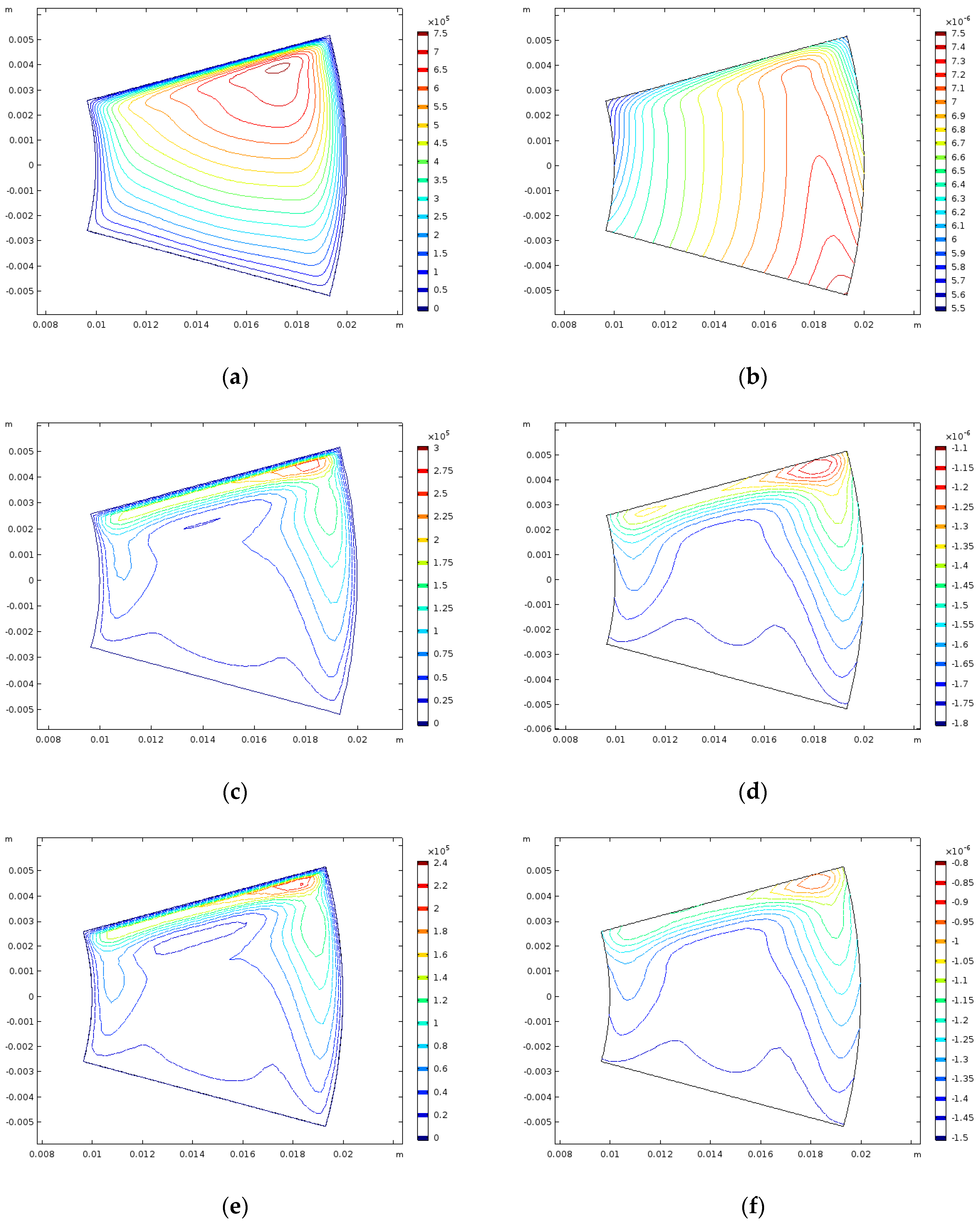
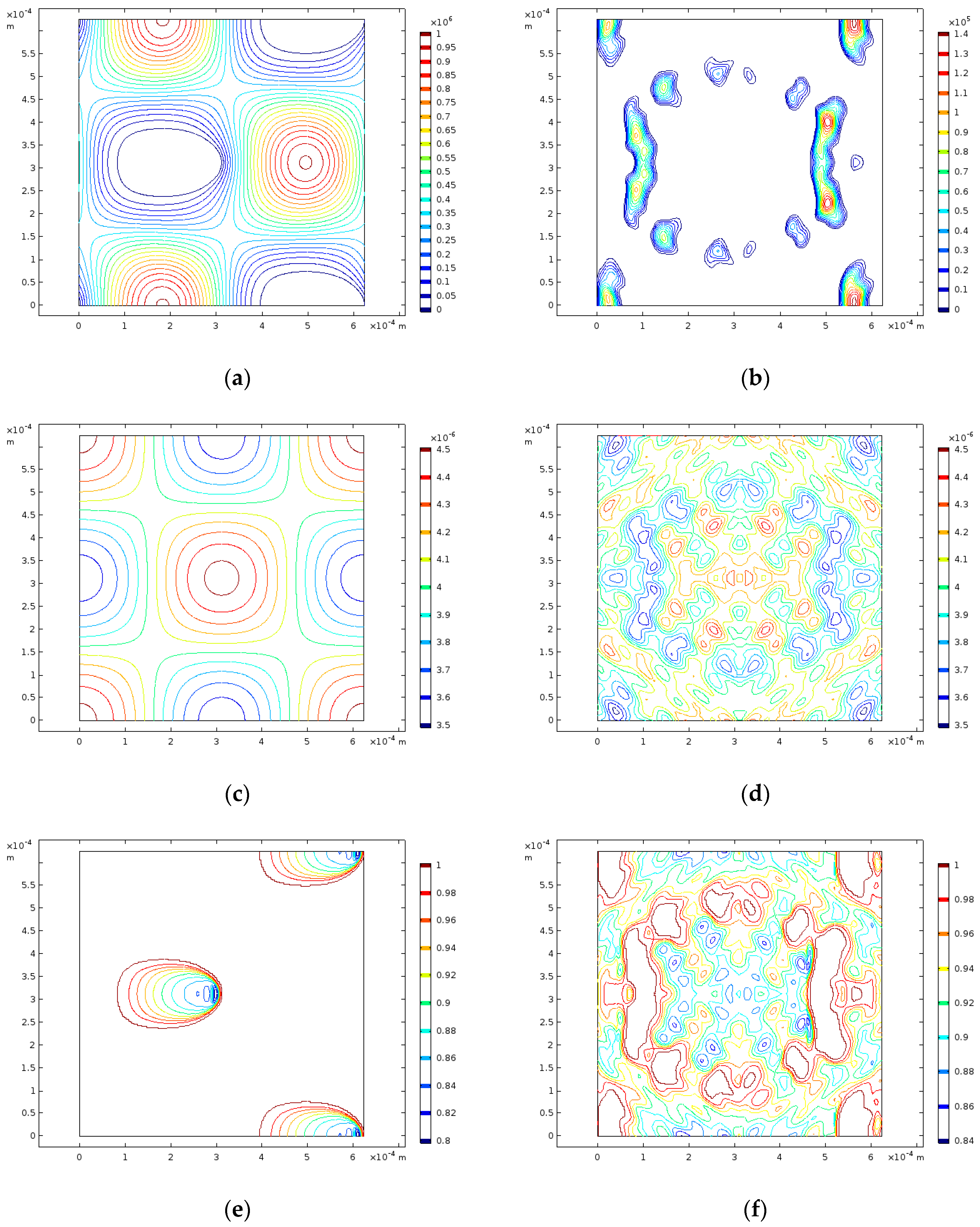
Using the two-scale method for EHL outlined results that were generated at the macro-scale, incorporating the effects of both the ideal and real topographies at the micro-scale. Figure 6a,b present the pressure and film thickness distributions for the case without topography. Subsequently, Figure 6c,d present the differences between the pressure and film thickness distributions without topography, and includes the ideal topography, and Figure 6e,f present the differences between the pressure and film thickness distributions without topography and includes the real topography. For all simulations considered in this section, the separation of scales was selected as $\epsilon =2^{-4}$ and the load $L=30$ N.

It is observed that there are significant differences in both the pressure and deformation distributions at the macro-scale when considering different topographies at the micro-scale. These differences are shown to be greater than the order of magnitude of the calculated values themselves. Figure 6c,e show that the ideal topography generates a larger difference in pressure than in the real topography when compared to the smooth surface case. This corresponds to a larger deviation of film thickness from the smooth surface case, as illustrated in Figure 6d,f. It is of note that the average trailing edge film thickness for the ideal and real topographies were found to be $H_{te}=9.12$ μm and $H_{te}=8.57$ μm, respectively, compared to $H_{te}=6.90$ μm for the case without topography. This demonstrates a stiffer response of the real topography, compared to the ideal, which is compounded by the pad becoming more out of shape (larger deformation of the pad surface). Overall these two observations lead to the hypothesis that a real surface topography leads to a significant difference in hydrodynamic performance, compared to an ideal one, and that neither of these solutions are represented well by smooth surface assumptions.

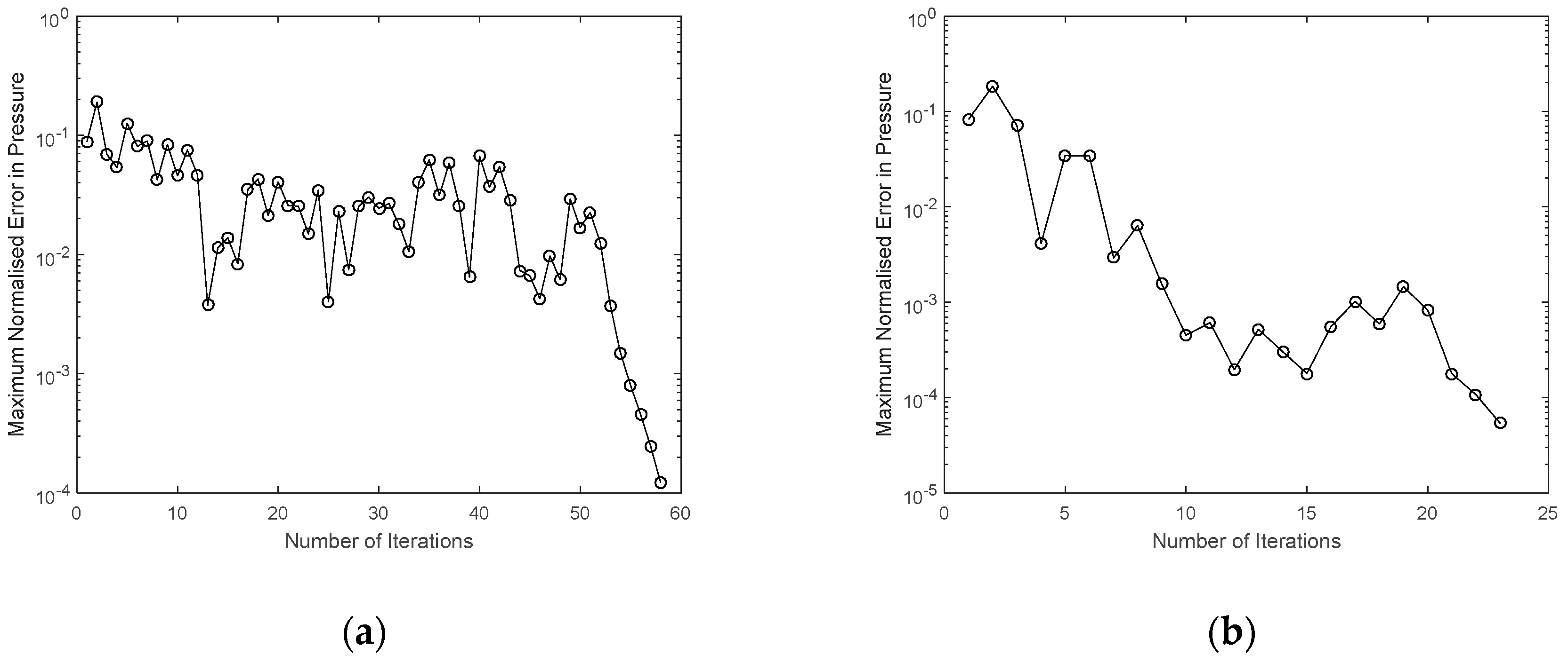
Convergence at the macro-scale was measured by the maximum normalized pressure between iterations of the solution procedure. The history of this criterion is given in Figure 7a,b for the two topographies investigated. It is seen that the real topography converges in less iterations than the ideal, and implies that deviations from the case without topography are smaller in this case. The convergence histories each demonstrate that the solutions generated are not trivial and require the iterative process outlined. As the initial solutions are updated, each iteration and the metamodels are concurrently modified and the results demonstrate the convergence of both the metamodel’s accuracy and macro-scale prediction.

3.4. Example Solutions of the Micro-EHL Model

To demonstrate the range of solutions generated at the micro-scale, as part of the macro-scale solution procedure, results are presented showing variations in the micro-scale pressure, film thickness, and the degree of saturation under different operating conditions. Two different conditions have been chosen as examples that highlight interesting micro-scale solutions, however, it should be noted that for any combination of the macro-scale parameters, it is possible to obtain similar micro-scale solutions. All results presented correspond to a scale separation of $\epsilon =2^{-4}$.

Figure 8a,c,e, respectively, show the micro-scale distributions of pressure, film thickness, and the degree of saturation for the ideal topography for the following parameters: $P=0$ Pa, $\frac{\partial P}{\partial X}=0$ Pa/m, $\frac{\partial P}{\partial Y}=0$ Pa/m, $H=4$ μm, $U=1$ m/s and $V=0$ m/s. Correspondingly, Figure 8b,d,f, respectively, show the micro-scale distributions of pressure, film thickness, and the degree of saturation for the real topography under the same conditions.

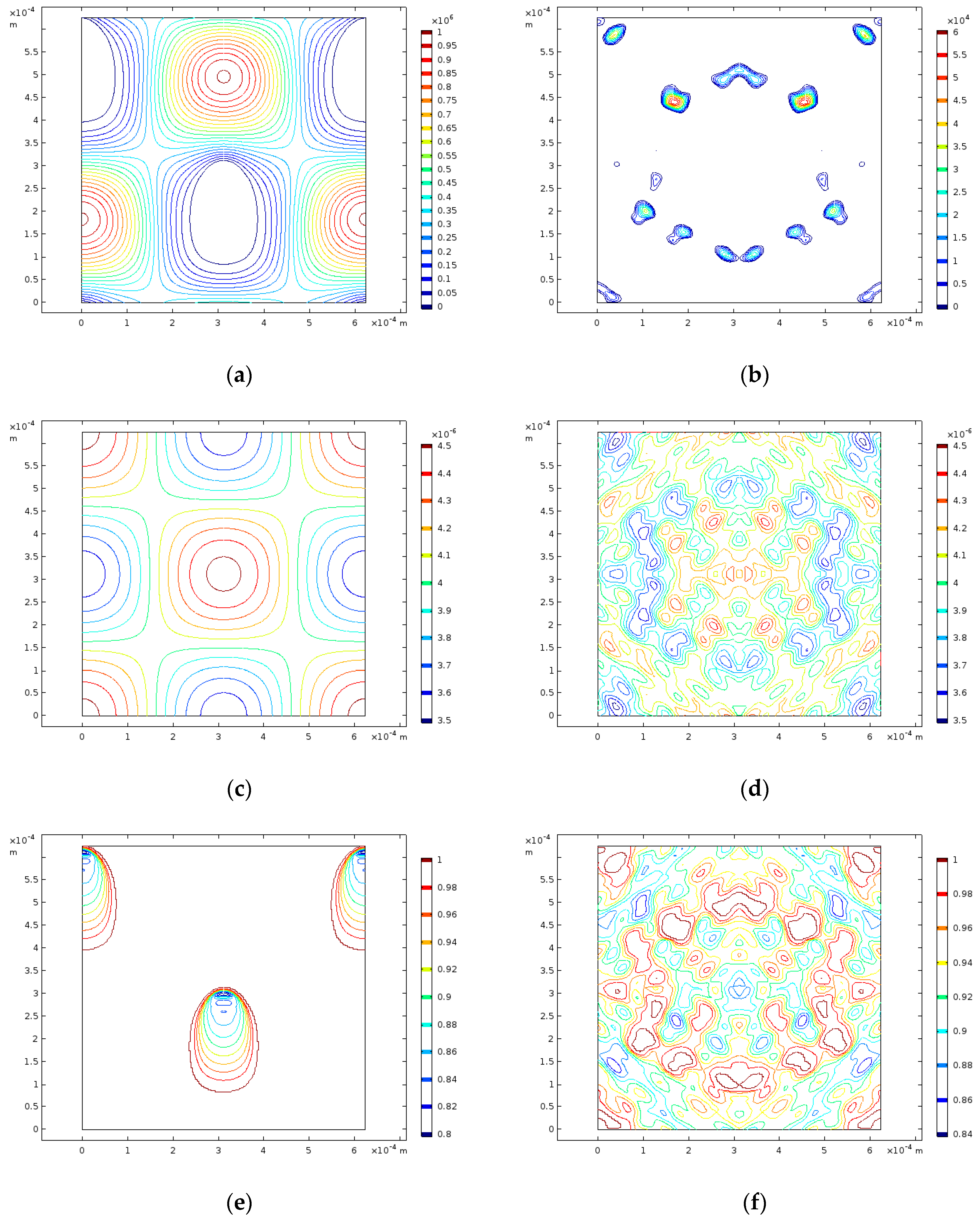
Figure 9a,c,e, respectively, show the micro-scale distributions of pressure, film thickness and the degree of saturation for the ideal topography for the following parameters: $P=0$ Pa, $\frac{\partial P}{\partial X}=0$ Pa/m, $\frac{\partial P}{\partial Y}=0$ Pa/m, $H=4$ μm, $U=0$ m/s and $V=1$ m/s. Correspondingly, Figure 9b,d,f, respectively, show the micro-scale distributions of pressure, film thickness and the degree of saturation for the real topography under the same conditions.

The distributions presented show that for the ideal topography there is an exact symmetry of the micro-scale pressure over the domain for both the conditions investigated. This generates a symmetry of the degree of saturation due to the direct coupling between the two variables. For the ideal topography, it is also shown that between the two sets of conditions presented in Figure 8 and Figure 9, there is a rotation of the pressure and degree of saturation solutions corresponding to the difference in velocity applied to each set of simulations. The film thickness distributions presented for the ideal topography are identical between the two conditions, which corresponds to the same average pressure over the domain in each of the results produced.

For the real topography, there is a smaller variation of pressure compared to the ideal topography for the same conditions imposed. Additionally, the plane of symmetry identified in the ideal case is also produced for the real case. This smaller variation in pressure is linked to the film thickness distributions, which have much larger scales in the ideal case than for the real case, this means that the pressure must vary significantly more than the ideal topographical features than the real topographical features. Further, in the real case, it is shown that the degree of saturation is distributed in a way that corresponds to the feature patterns described by the film thickness and this complexity is linked to how pressure is distributed over the surface features. Again, for the real case, there is no significant difference between the film thicknesses under each of the conditions because the average pressures are similar. However, unlike the ideal case, there is no direct rotation of the solutions with the direction of velocity, this is linked to the complexity of the flow as it passes over the real surface features, as compared to the flow over ideal surface features.

Overall, the example micro-scale solutions demonstrate the difference between models inclusive of surface topography and cavitation, as compared to the smooth surface assumptions used to define the macro-scale model. The homogenization of parameters at the micro-scale links directly to the values implemented in the macro-scale model, mapping the differences illustrated in this section to that described in the bearing mechanics.

3.5. Metamodeling

To determine the effectiveness of the metamodel in predicting the micro-scale data at the macro-scale, a check was performed at various locations on the pad for both the ideal and real topographies. These points were selected arbitrarily as the center of the pad and the locations of (macro-scale) maximum pressure and minimum film thickness in the case without topography. This check compared the percentage difference between the metamodel predictions at the macro-scale by the metamodels (as presented in Section 3.3) to the exact values obtained at the micro-scale. The results of this study are given in

Table 3. Comparison of metamodel predictions and exact micro-scale values for the ideal topography.

Parameter						% Difference in
$\mathit{P}$ (MPa)	$\frac{\partial \mathit{P}}{\partial \mathit{X}}$ (MPa/mm)	$\frac{\partial \mathit{P}}{\partial \mathit{Y}}$ (MPa/mm)	$\mathit{H}$ (μm)	$\mathit{U}$ (m/s)	$\mathit{V}$ (m/s)	${\mathit{Q}}_{\mathit{X}}$	${\mathit{Q}}_{\mathit{Y}}$	${\mathit{P}}^{*}$
0.43	0.02	−0.05	8.31	0	0.77	0.321	0.103	−0.450
0.65	−0.03	0.03	8.23	−0.16	0.89	0.873	−0.611	0.047
0	0.13	−0.13	7.28	−0.18	0.53	−0.009	0.057	−0.413

for the ideal topography and

Table 4. Comparison of metamodel predictions and exact micro-scale values for the real topography.

Parameter						% Difference in
$\mathit{P}$ (MPa)	$\frac{\partial \mathit{P}}{\partial \mathit{X}}$ (MPa/mm)	$\frac{\partial \mathit{P}}{\partial \mathit{Y}}$ (MPa/mm)	$\mathit{H}$ (μm)	$\mathit{U}$ (m/s)	$\mathit{V}$ (m/s)	${\mathit{Q}}_{\mathit{X}}$	${\mathit{Q}}_{\mathit{Y}}$	${\mathit{P}}^{*}$
0.41	0.02	−0.05	8.12	0	0.77	0.230	−0.133	0.786
0.67	−0.04	0.03	8.04	−0.16	0.89	0.505	0.055	−0.308
0	0.27	−0.33	7.05	−0.18	0.53	−0.701	0.802	0.017

for the real topography. Both results show that the metamodel predictions are with 1% of the actual values for all the cases and topographies considered. This is an improvement in performance as compared to previous works [39], despite an increase in dimensionality of the problem, which is attributed to the curvilinear discretization and DOE checks conducted as part of this study.

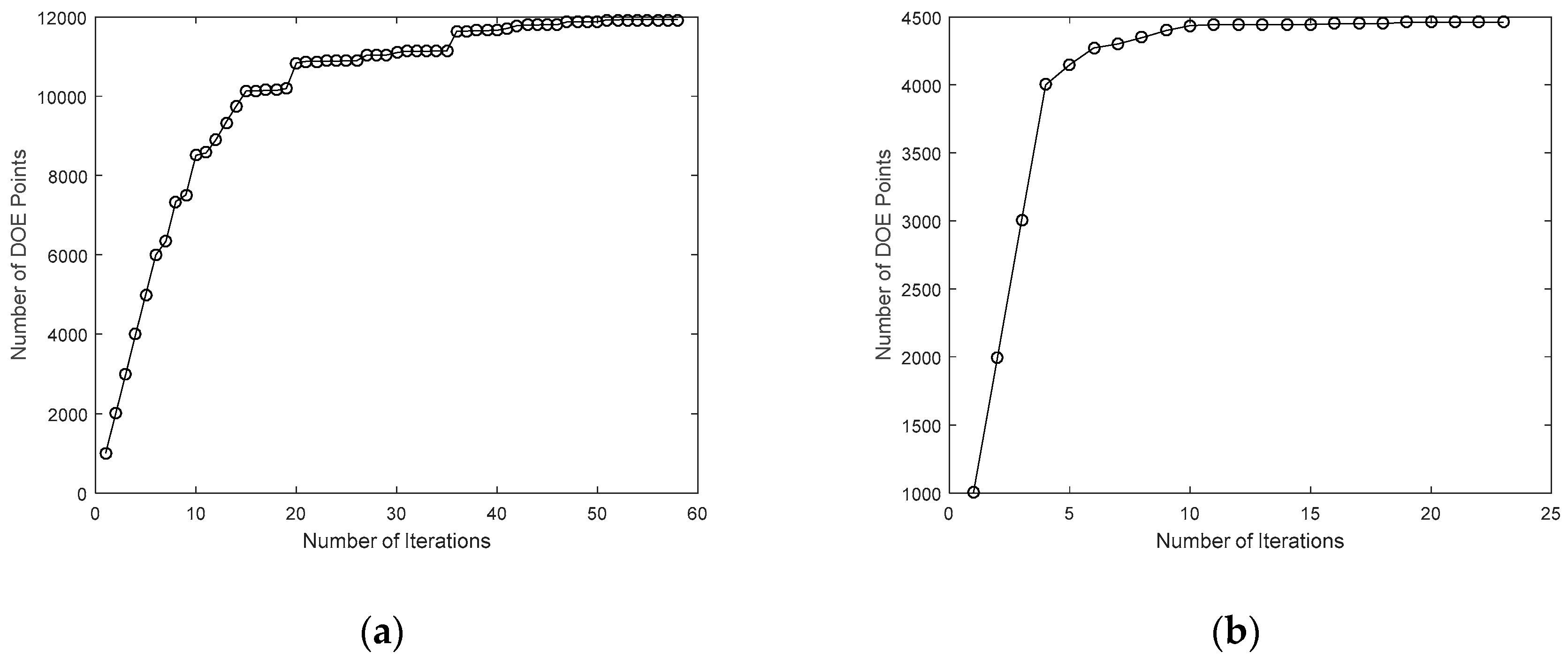
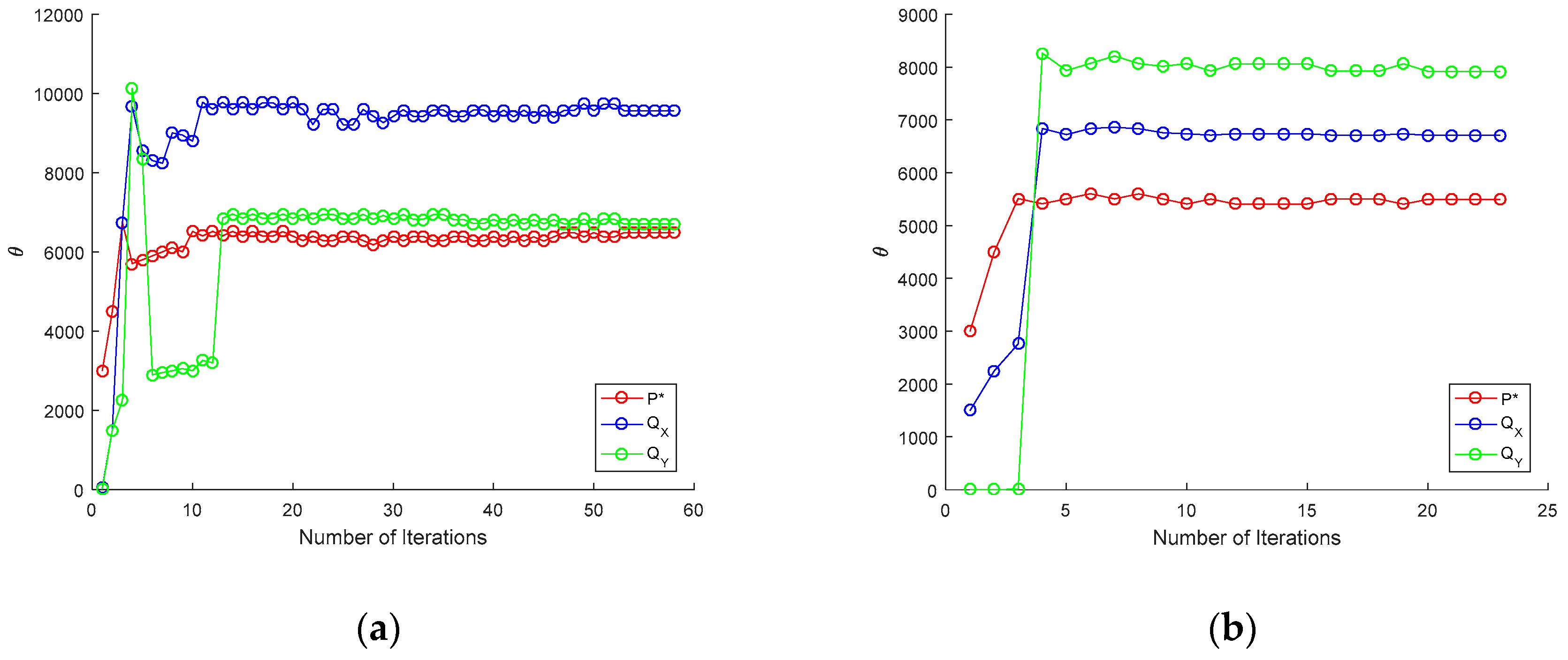
A further study was conducted to analyze the performance of the metamodeling as part of the macro-scale solution procedure. Figure 10a,b show the variation of the size of the DOE with the number of macro-scale iterations for the ideal and real topographies, respectively. Correspondingly, Figure 11a,b show the change in metamodel closeness of fit parameters with the number of macro-scale iterations for the different topographies.

As the macro-scale solution procedure progresses and the solvers reach convergence in the pressure field, there is also convergence in both the size of the DOE and the closeness of fit parameters. Throughout the first few iterations, the size of the DOE growth is reasonably linear, with almost the full 1000 points added each instance; as the pressure field converges, the solutions on each iteration are closer together and therefore less data points are added. In these cases, the total number of DOE points was significantly different with 11,930 needed for the ideal topography case and 4462 for the real topography case, this is the result of many more iterations being required in the ideal case. The closeness of fit parameters are shown to change significantly over the first few iterations, but as the pressure field converges, so do each of the $\theta$ values, corresponding to the number of DOE points reaching a steady value. When no points are added to the DOE, the closeness of fit parameters remains unchanged.

4. Discussion

In this article, a two-scale method for modelling surface topography in the EHL of tilted-pad bearings is derived. The approach is based on the HMM and facilitates the homogenized effects of micro-EHL to be coupled into the macro-EHL mechanics using flow factors generated from metamodeling techniques. This work furthers the methods previously investigated by the authors in order to include three-dimensional bearings and a direct comparison of ideal and real surface topographies.

A study was conducted comparing the results generated by the two-scale method with those presented by Almqvist [22] under hydrodynamic conditions. Results were given for two different values of the separation of scale parameters $\epsilon$ considering the ideal topography. Macro-scale pressure distributions compared directly to those of Almqvist [22] and were identical for the different separation of scales examined. This verified the two-scale method for modelling surface topography under hydrodynamic conditions against the well-established approach in the literature and the scope for the method to analyze EHL, inclusive of the homogenized effects of surface topography.

The choice of macro-scale EHL model was verified by comparing results generated by simulations including the pad and collar together against simulations of the pad alone. This was undertaken to determine the significance of implementing a zero-deformation boundary condition on the pad backing. The ratio of backing to the pad average deformation was shown to increase with a ratio of backing to pad thickness such that the thinner pads generated larger backing deformations. The backing thickness was chosen as $t_b=10$ mm and the pad thickness $t_p=2$ mm, where the ratio of pad to backing average deformation was 0.01. This influence of the backing deformation was assumed to be small enough to be neglected in the remainder of EHL studies conducted and a zero-deformation boundary condition for the backing was used. For larger loads and thinner pads, this assumption cannot be made and the full pad and collar model must be simulated to correctly describe the deformation in the bearing.

Macro-scale EHL simulations were carried out that compared the results generated without topography to those inclusive of the effects of the homogenized ideal and real topographies by the two-scale method. Simulations including the ideal topography generated larger differences in pressure and film thickness than the simulations including the real topography. Additionally, the average trailing edge film thickness deviated further in the ideal case than the real case from that without topography. Overall this demonstrated a stiffer response of those simulations inclusive of the real topography in comparison to those inclusive of the ideal topography under the conditions. It is hypothesized that the real topography has a stiffer response and this generates a better performing hydrodynamic wedge in comparison to the ideal topography, which leads to an improved load carrying capacity for the bearing.

Micro-scale EHL simulations were undertaken to demonstrate the range of solutions generated at this scale when including surface topography, the examples selected were representative of conditions at the macro-scale and illustrated interesting solutions. Periodicity in the distributions of pressure, film thickness, and the degree of saturation was demonstrated and satisfied the assumptions of the HMM underlying the two-scale method. Symmetry in the solutions under both ideal and real conditions were also observed owing to the periodicity required and the conditions imposed. The responses of the real topography showed more variation compared to the ideal topography and was shown to relate to the difference in complexity of the surface features. However, in the ideal case, the difference in pressure was much larger than the real case, owing to the larger scales of the surface features.

An analysis of the metamodeling techniques used to couple the scales of the problem was also undertaken. A check of the macro-scale EHL solutions generated by the metamodels was compared to the exact values obtained at the micro-scale. Four different locations on the pad surface were chosen, and for both the ideal and real surface topographies, there was no difference of more than 1% between them. It was also demonstrated that as the macro-scale solution procedure progressed, there was almost a linear increase in the size of the DOE used, meaning that the intermediate solutions differ significantly from the previous iterations. As the size of the DOE is increased and more is known about the design space then the intermediate solutions become closer together and less points are added. Eventually the sizes converge, which also corresponds to convergence in the macro-scale distributions, and the closeness of fit parameters used in tuning the metamodel response. Overall the metamodeling procedure was shown to be more accurate and efficient than implementations in previous works [39], despite the increase in dimensionality.

5. Conclusions

The two-scale method for tilted-pad bearings derived in this paper facilitates the homogenized effects of surface topography at the micro-scale to be modeled at the macro-scale. The method is based on the HMM and furthers past studies [36,37,38,39,40] to include a three-dimensional bearing and a comparison of the ideal and real surface topographies. Results showed that the two-scale method compared well to the established literature in modeling hydrodynamic lubrication [22] and the pad can be modeled without the backing under EHL conditions when the ratio of pad to backing thickness and load capacity are suitably chosen. Macro-scale EHL results demonstrated a stiffer response of the real topography than the ideal topography when compared to the case without. It was hypothesized that this mechanism could explain why such surfaces lead to a better hydrodynamic performance than in the without or ideal topography case. Micro-scale EHL results illustrated the significant differences in flow features for the two topographies considered and that the distributions generated at this scale are consistent with the assumptions of the HMM. Metamodeling solutions showed how the size of the DOE increased with the progression of the macro-scale solution procedure, and that, as convergence was reached in the resulting distributions, there was also convergence in the size of the DOE and the metamodel tuning parameters.

The method derived will be furthered to analyze additional flow phenomena conventionally examined in lubricated contacts—such as compressibility, piezoviscosity, and non-Newtonian behavior of the lubricant, as well as including derivatives across the film and inertial effects. All of which have previously been included for line contact problems [38,40]. Surface topography will be parameterized and the effects on homogenized variables will be analyzed across the scales; this will allow macro-scale variations in topography and the performance of different surface features to be parametrically compared using the approach.

References

1. Dowson, D. History of Tribology; Addison-Wesley Longman Limited: Boston, MA, USA, 1979. [Google Scholar]
2. Srikanth, D.; Chaturvedi, K.; Reddy, A. Modelling of large tilting pad thrust bearing stiffness and damping coefficients. Tribol. Ind. 2009, 31, 2–28. [Google Scholar]
3. Nicoletti, R.; Santos, I.F. Frequency response analysis of an actively lubricated rotor/tilting-pad bearing system. J. Eng. Gas Turbines Power 2005, 127, 638–645. [Google Scholar] [CrossRef]
4. Markin, D.; McCarthy, D.; Glavatskih, S. A FEM approach to simulation of tilting-pad thrust bearing assemblies. Tribol. Int. 2003, 36, 807–814. [Google Scholar] [CrossRef]
5. Etsion, I. State of the art in laser surface texturing. J. Tribol. 2005, 127, 248–253. [Google Scholar] [CrossRef]
6. Greenwood, J.; Johnson, K. The behaviour of transverse roughness in sliding elastohydrodynamically lubricated contacts. Wear 1992, 153, 107–117. [Google Scholar] [CrossRef]
7. Hooke, C.J. Surface roughness modification in elastohydrodynamic line contacts operating in the elastic piezoviscous regime. J. Eng. Tribol. 1998, 212, 145–162. [Google Scholar] [CrossRef]
8. Venner, C.H.; Morales-Espejel, G.E. Amplitude reduction of small-amplitude waviness in transient elastohydrodynamically lubricated line contacts. J. Eng. Tribol. 1999, 213, 487–504. [Google Scholar] [CrossRef]
9. Mourier, L.; Mazuyer, D.; Ninove, F.; Lubrecht, A. Lubrication mechanisms with laser-textured surfaces in elastohydrodynamic regime. Proc. Inst. Mech. Eng. Part J. 2010, 224, 697–711. [Google Scholar] [CrossRef]
10. Gao, L.; Yang, P.; Dymond, I.; Fisher, J.; Jin, Z. Effect of surface texturing on the elastohydrodynamic lubrication analysis of metal-on-metal hip implants. Tribol. Int. 2010, 43, 1851–1860. [Google Scholar] [CrossRef]
11. Felix-Quinonez, A.; Ehret, P.; Summers, J. On three-dimensional flat-top defects passing through an EHL point contact: A comparison of modeling with experiments. J. Tribol. 2005, 127, 51–60. [Google Scholar] [CrossRef]
12. Bonaventure, J.; Cayer-Barrioz, J.; Mazuyer, D. Transition between mixed lubrication and elastohydrodynamic lubrication with randomly rough surfaces. Tribol. Lett. 2016. [Google Scholar] [CrossRef]
13. Vakis, A.; Yastrebov, V.; Scheibert, J.; Minfray, C.; Nicola, L.; Dini, D.; Almqvist, A.; Paggi, M.; Lee, S.; Limbert, G. Modeling and simulation in tribology across scales: An overview. Tribol. Int. 2018. [Google Scholar] [CrossRef]
14. Tzeng, S.; Saibel, E. Surface roughness effect on slider bearing lubrication. Asle Trans. 1967, 10, 334–348. [Google Scholar] [CrossRef]
15. Christensen, H. Stochastic models for hydrodynamic lubrication of rough surfaces. Proc. Inst. Mech. Eng. 1969, 184, 1013–1026. [Google Scholar] [CrossRef]
16. Elrod, H.G. Thin-film lubrication theory for Newtonian fluids with surfaces possessing striated roughness or grooving. J. Lubr. Technol. 1973, 95, 484–489. [Google Scholar] [CrossRef]
17. Patir, N.; Cheng, H. An average flow model for determining effects of three-dimensional roughness on partial hydrodynamic lubrication. Trans. ASME, J. Lubr. Technol. 1978, 100, 12–17. [Google Scholar] [CrossRef]
18. Patir, N.; Cheng, H. Application of average flow model to lubrication between rough sliding surfaces. Trans. ASME J. Lubr. Technol. 1979, 101, 220–229. [Google Scholar] [CrossRef]
19. Almqvist, A.; Dasht, J. The homogenization process of the Reynolds equation describing compressible liquid flow. Tribol. Int. 2006, 39, 994–1002. [Google Scholar] [CrossRef]
20. Sahlin, F.; Almqvist, A.; Larsson, R.; Glavatskih, S. Rough surface flow factors in full film lubrication based on a homogenization technique. Tribol. Int. 2007, 40, 1025–1034. [Google Scholar] [CrossRef]
21. Larsson, R. Modelling the effect of surface roughness on lubrication in all regimes. Tribol. Int. 2009, 42, 512–516. [Google Scholar] [CrossRef]
22. Almqvist, A. Homogenization of the Reynolds equation governing hydrodynamic flow in a rotating device. J. Tribol. 2011. [Google Scholar] [CrossRef]
23. Almqvist, A.; Fabricius, J.; Lundström, T.S.; Wall, P. Flow in thin domains with a microstructure: Lubrication and thin porous media. AIP Conf. Proc. 2017. [Google Scholar] [CrossRef]
24. de Kraker, A.; van Ostayen, R.; Rixen, D. Development of a texture averaged Reynolds equation. Tribol. Int. 2010, 43, 2100–2109. [Google Scholar] [CrossRef]
25. Bou-Saïd, B.; Tichy, J. On the transition from Reynolds to Stokes roughness. In Transient Processes in Tribology, Proceedings of the 30th Leeds-Lyon Symposium on Tribiology, Lyon, France, 2–5 September 2003; Lubrecht, A., Dalmaz, G., Eds.; Elsevier: Amsterdam, The Netherlands, 2004. [Google Scholar]
26. Martin, S. Influence of multiscale roughness patterns in cavitated flows: Applications to journal bearings. Math. Probl. Eng. 2008, 2008, 1–26. [Google Scholar] [CrossRef]
27. Scaraggi, M.; Carbone, G.; Persson, B.N.J.; Dini, D. Lubrication theory in soft rough contacts: A novel homogenization approach. Part I—Theory. Soft Matter. 2011, 7, 10395–10406. [Google Scholar] [CrossRef] [Green Version]
28. Scaraggi, M.; Carbone, G.; Dini, D. Lubrication theory in soft rough contacts: A novel homogenization approach. Part II—Discussion. Soft Matter. 2011, 7, 10407–10416. [Google Scholar] [CrossRef]
29. Almqvist, A.; Fabricius, J.; Spencer, A.; Wall, P. Similarities and differences between the flow factor method by Patir and Cheng and homogenization. J. Tribol. 2011, 133, 031702. [Google Scholar] [CrossRef]
30. Almqvist, A.; Wall, P. Homogenization of the Reynolds equation. In Encyclopedia Tribology; Springer: Berlin/Heidelberg, Germany, 2013; pp. 1685–1690. [Google Scholar]
31. Bayada, G.; Cid, B.; Vázquez, C. Two-scale homogenization study of a Reynolds-rod elastohydrodynamic model. Math. Models Methods Appl. Sci. 2003, 13, 259–293. [Google Scholar] [CrossRef]
32. Scheichl, B.; Paleotti, F.S.G. Elasto-hydrodynamic lubrication of rough contacts: On a rigorous generalisation of the homogenisation approach. In Proceedings of the European Congress on Computational Methods in Applied Sciences and Engineering, Vienna, Austria, 10–14 September 2012. [Google Scholar]
33. Budt, M.; Temizer, I.; Wriggers, P. A computational homogenization framework for soft elastohydrodynamic lubrication. Comput. Mech. 2012, 49, 749–767. [Google Scholar] [CrossRef] [Green Version]
34. E, W.; Engquist, B. The heterognous multiscale methods. Commun. Math. Sci. 2003, 1, 87–132. [Google Scholar] [CrossRef]
35. E, W.; Engquist, B. The heterogeneous multi-scale method for homogenization problems. In Multiscale Methods in Science and Engineering; Springer: Berlin/Heidelberg, Germany, 2005; pp. 89–110. [Google Scholar]
36. Gao, L.; Hewson, R. A multiscale framework for EHL and micro-EHL. Tribol. Trans. 2012, 55, 713–722. [Google Scholar] [CrossRef]
37. de Boer, G.; Hewson, R.; Thompson, H.; Gao, L.; Toropov, V. Two-scale EHL: Three-dimensional topography in tilted-pad bearings. Tribol. Int. 2014, 79, 111–125. [Google Scholar] [CrossRef] [Green Version]
38. de Boer, G.; Gao, L.; Hewson, R.; Thompson, H.; Raske, N.; Toropov, V. A multiscale method for optimising surface topography in elastohydrodynamic lubrication (EHL) using metamodels. Struct. Multidiscip. Optim. 2016, 54, 483–497. [Google Scholar] [CrossRef] [Green Version]
39. de Boer, G.; Gao, L.; Hewson, R.; Thompson, H. Heterogeneous Multiscale Methods for modelling surface topography in Elastohydrodynamic Lubrication line contacts. Tribol. Int. 2017, 113, 262–278. [Google Scholar] [CrossRef] [Green Version]
40. Gao, L.; de Boer, G.; Hewson, R. The role of micro-cavitation on EHL: A study using a multiscale mass conserving approach. Tribol. Int. 2015, 90, 324–331. [Google Scholar] [CrossRef] [Green Version]
41. Pérez-Ràfols, F.; Larsson, R.; van Riet, E.J.; Almqvist, A. On the loading and unloading of metal-to-metal seals: A two-scale stochastic approach. Proc. Inst. Mech. Eng. Part J. 2017. [Google Scholar] [CrossRef]
42. Elrod, H.G. A cavitation algorithm. Trans. ASME J. Lubr. Technol. 1981, 103, 350. [Google Scholar] [CrossRef]
43. Almqvist, A.; Fabricius, J.; Larsson, R.; Wall, P. A new approach for studying cavitation in lubrication. J. Tribol. 2014, 136, 011706. [Google Scholar] [CrossRef]
44. Giacopini, M.; Fowell, M.T.; Dini, D.; Strozzi, A. A mass-conserving complementarity formulation to study lubricant films in the presence of cavitation. J. Tribol. 2010, 132, 041702. [Google Scholar] [CrossRef]
45. Pérez-Ràfols, F.; Wall, P.; Almqvist, A. On compressible and piezo-viscous flow in thin porous media. Proc. R. Soc. A 2018, 474, 20170601. [Google Scholar] [CrossRef] [PubMed] [Green Version]
46. de Boer, G.; Dowson, D. An Arbitrary Lagrangian–Eulerian Formulation for Modelling Cavitation in the Elastohydrodynamic Lubrication of Line Contacts. Lubricants 2018, 6, 13. [Google Scholar] [CrossRef]
47. Söderfjäll, M.; Larsson, R.; Marklund, P.; Almqvist, A. Texture-induced effects causing reduction of friction in mixed lubrication for twin land oil control rings. J. Eng. Tribol. 2018, 232, 166–178. [Google Scholar] [CrossRef]
48. Comsol Inc., USA. Comsol Multiphysics 5.3a [Computer Software]. 2018. Available online: https://www.comsol.com/ (accessed on 29 June 2018).
49. The MathsWorks Inc., USA. Matlab vR2018 [Computer Software]. 2018. Available online: https://www.mathsworks.com/ (accessed on 29 June 2018).
Figure 1. Macro-scale geometry showing the periodic section of a tri-pad tilted-pad bearing.
Lubricants 06 00078 g001
Figure 2. Macro-scale solid mechanics boundary conditions for: (a) Case (i), the backing and pad modelled together; and (b) Case (ii), the pad modelled alone.
Lubricants 06 00078 g002
Figure 3. Macro-scale pressure distributions (Pascals) on the pad surface under hydrodynamic conditions including an ideal surface topography. (a) ε = 2 4 ; and (b) ε = 2 5 .
Lubricants 06 00078 g003
Figure 4. (a) Ratio of backing to pad average deformations presented as a function of the ratio of backing to pad thicknesses. (b) Visualisation of the deformation (meters) on the pad and backing model, scaled by a factor of 500 and mirrored about the axial line of symmetry.
Lubricants 06 00078 g004
Figure 5. Deformation of the pad surface (meters) under EHL conditions without topography: (a) L = 10 N; (b) L = 30 N.
Lubricants 06 00078 g005
Figure 6. Distributions of macro-scale solutions showing: (a) pressure (Pascals) without topography; (b) film thickness (meters) without topography; (c) difference in pressure between (a) and the case with ideal topography; (d) difference in film thickness between (b) and the case with ideal topography; (e) difference in pressure between (a) and the case with real topography; and (f) difference in film thickness between (a) and the case with real topography.
Lubricants 06 00078 g006
Figure 7. Convergence of the macro-scale solver for: (a) the ideal topography; and (b) the real topography.
Lubricants 06 00078 g007
Figure 8. Distributions of micro-scale solutions for P = 0 Pa, P X = 0 Pa/m, P Y = 0 Pa/m, H = 4 μm, U = 1 m/s and V = 0 m/s: (a) pressure (Pascals), ideal topography; (b) pressure (Pascals), real topography; (c) film thickness (meters), ideal topography; (d) film thickness (meters), real topography; (e) degree of saturation, ideal topography; and (f) degree of saturation, real topography.
Lubricants 06 00078 g008
Figure 9. Distributions of micro-scale solutions for P = 0 Pa, P X = 0 Pa/m, P Y = 0 Pa/m, H = 4 μm, U = 0 m/s and V = 1 m/s: (a) pressure (Pascals), ideal topography; (b) pressure (Pascals), real topography; (c) film thickness (meters), ideal topography; (d) film thickness (meters), real topography; (e) degree of saturation, ideal topography; and (f) degree of saturation, real topography.
Lubricants 06 00078 g009
Figure 10. Variation of the size of the DOE with the number of macro-scale iterations for: (a) the ideal topography; and (b) the real topography.
Lubricants 06 00078 g010
Figure 11. Variation of the metamodel closeness of fit parameters with the number of macro-scale iterations for: (a) the ideal topography; and (b) the real topography.
Lubricants 06 00078 g011