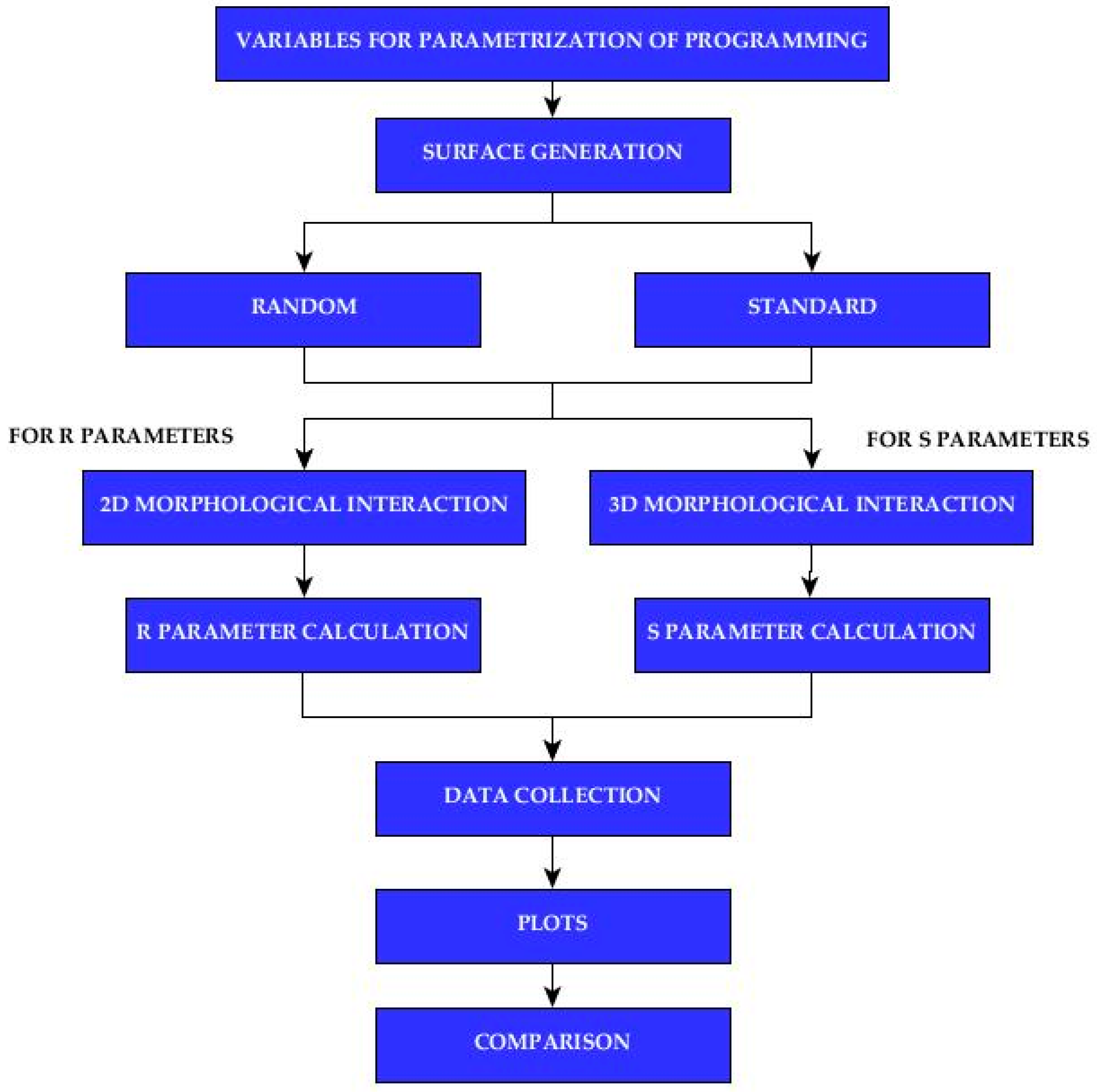
Figure 1.
Flowchart of the developed program.
Figure 1.
Flowchart of the developed program.
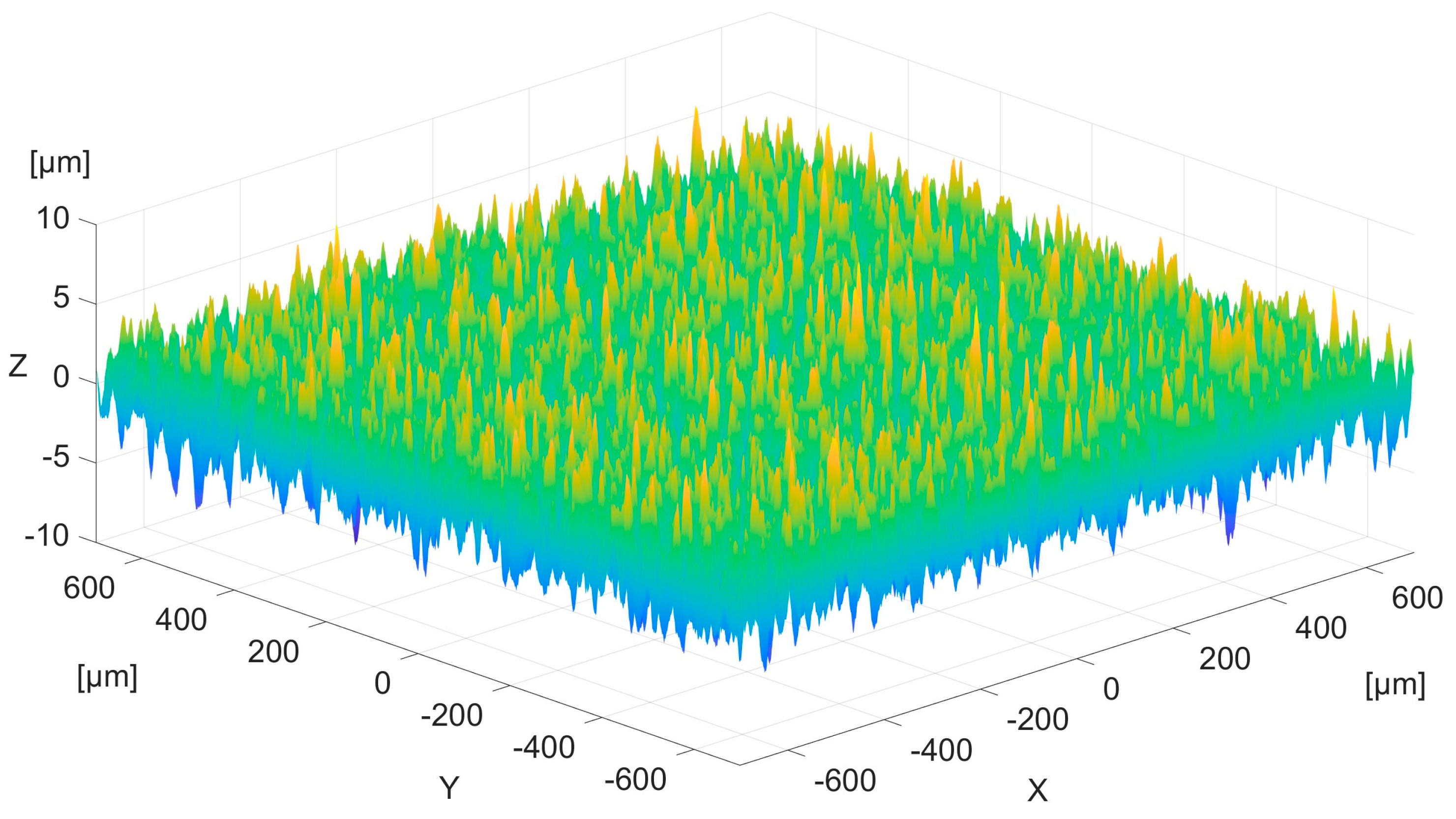
Figure 2.
The point cloud generated. Z (height in µm), X, and Y (horizontal displacement in µm).
Figure 2.
The point cloud generated. Z (height in µm), X, and Y (horizontal displacement in µm).
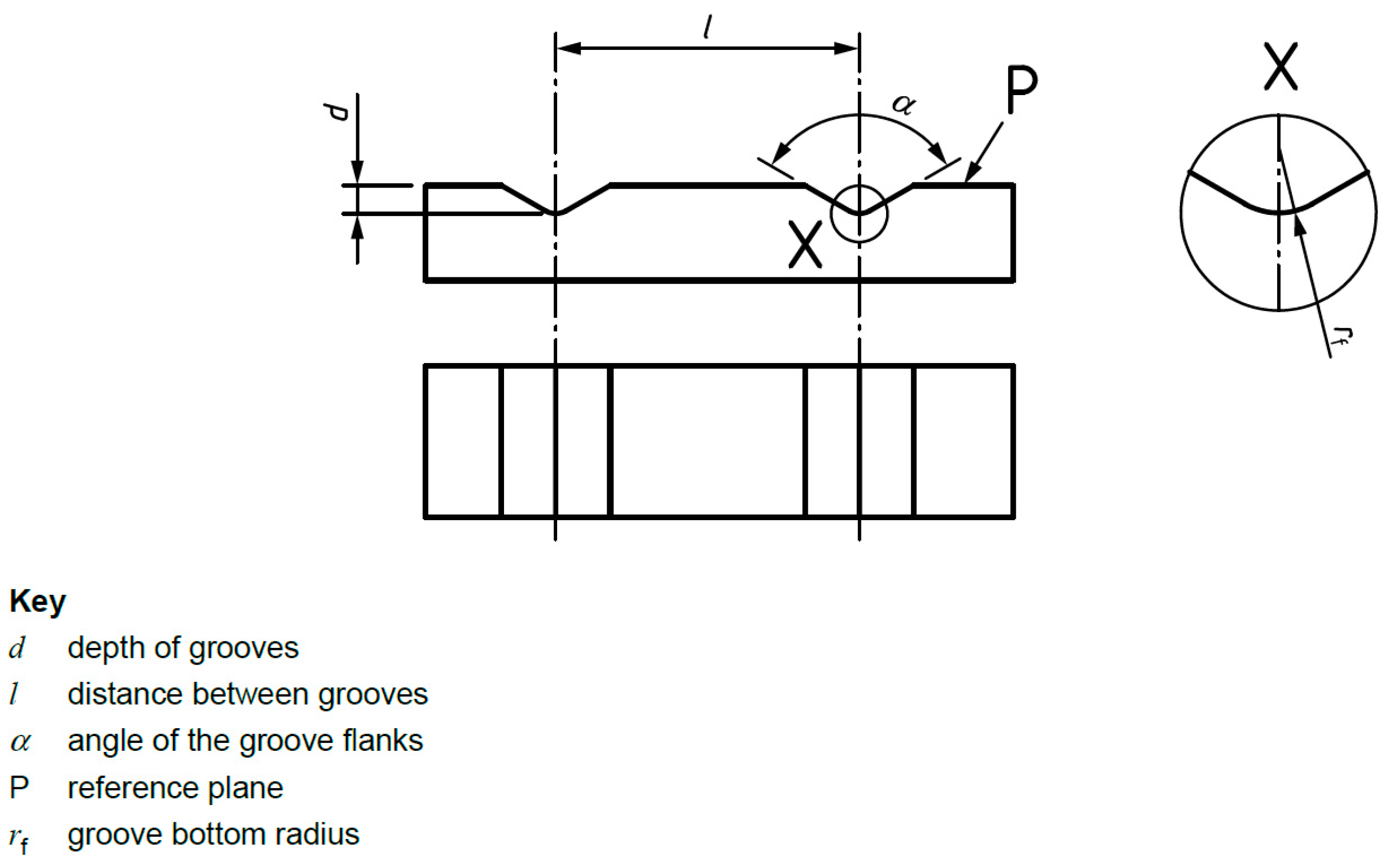
Figure 3.
The two-parallel-grooves standard (ER1) of the UNE-EN ISO 25178-701:2011 [
30] standard.
Figure 3.
The two-parallel-grooves standard (ER1) of the UNE-EN ISO 25178-701:2011 [
30] standard.
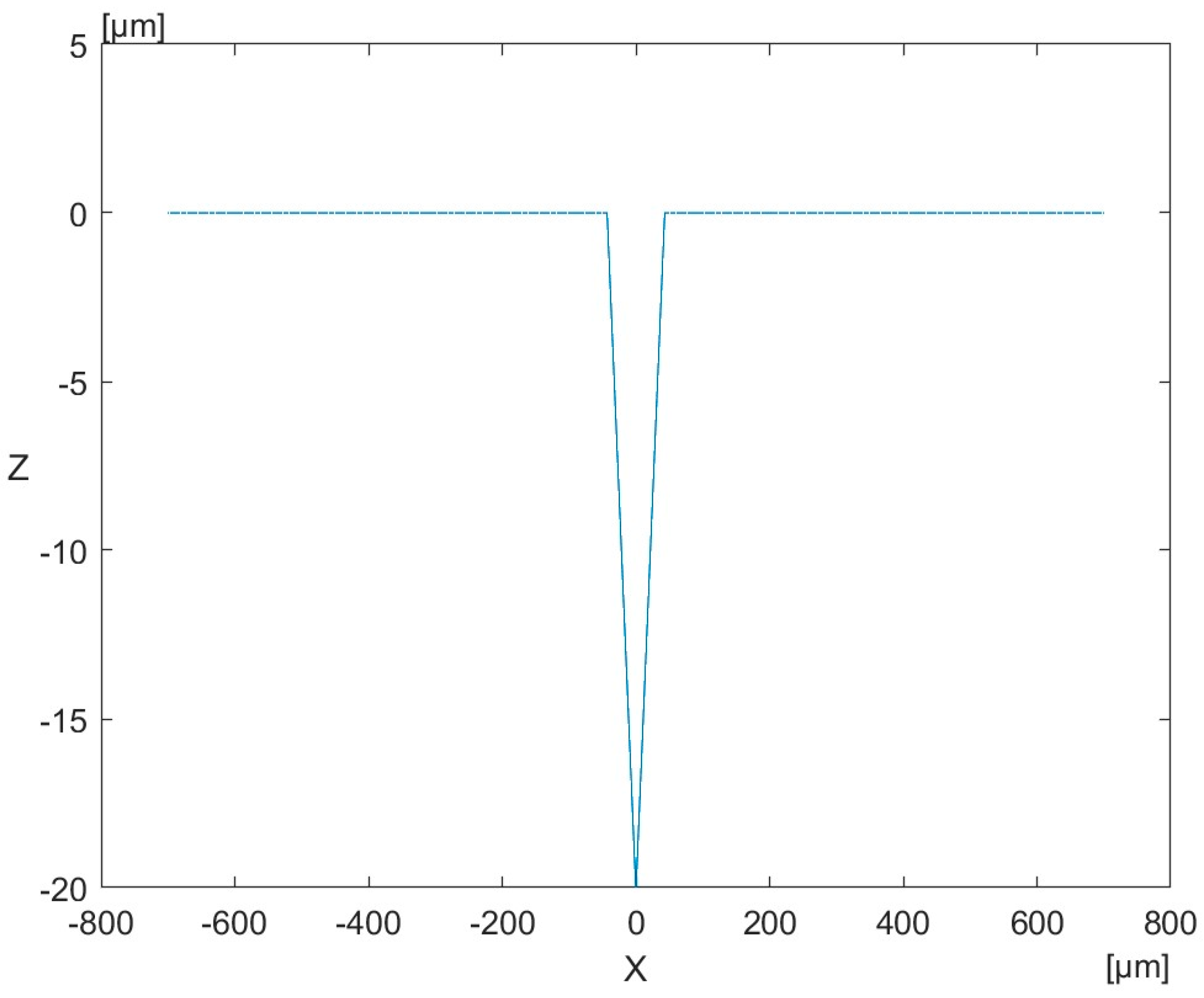
Figure 4.
Profile of the groove standard. Z (height in µm) and X (Horizontal displacement in µm).
Figure 4.
Profile of the groove standard. Z (height in µm) and X (Horizontal displacement in µm).
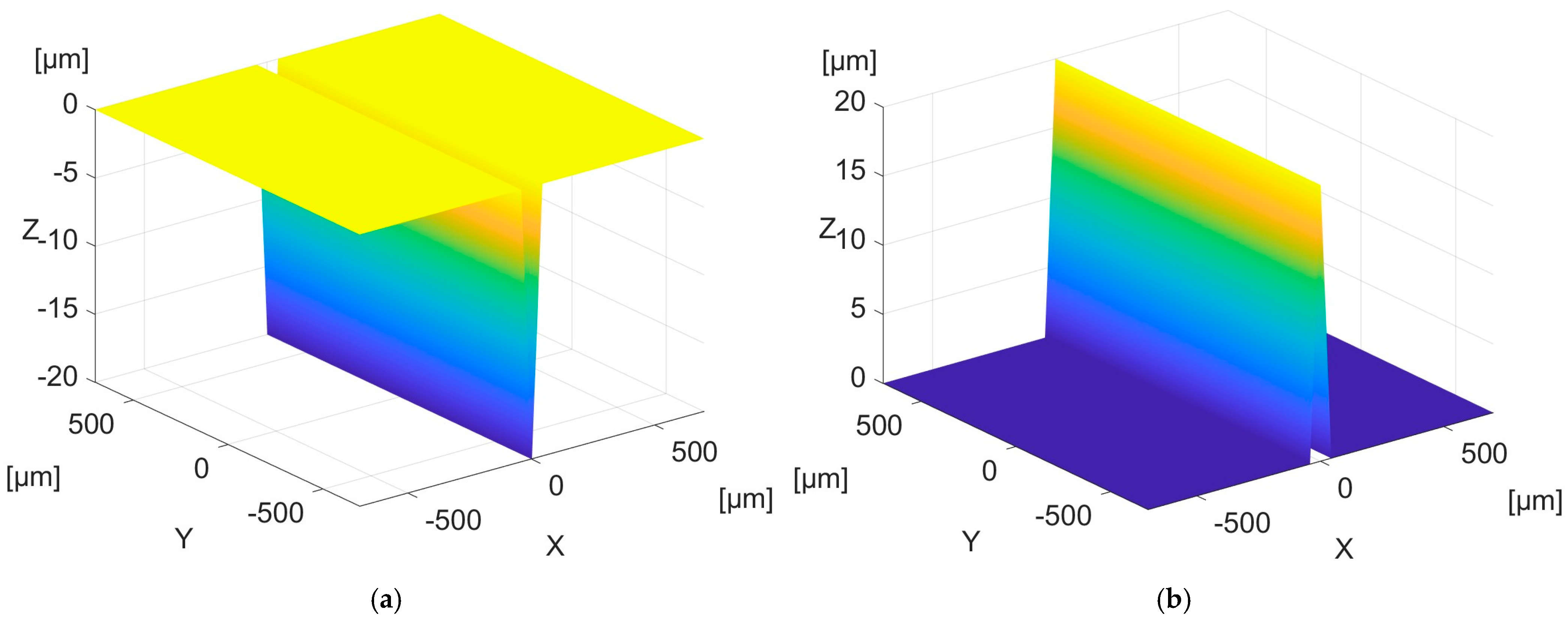
Figure 5.
(a) Groove standard. Z (height in µm), X, and Y (horizontal displacement in µm). (b) Triangular peak standard. Z (height in µm), X, and Y (horizontal displacement in µm).
Figure 5.
(a) Groove standard. Z (height in µm), X, and Y (horizontal displacement in µm). (b) Triangular peak standard. Z (height in µm), X, and Y (horizontal displacement in µm).
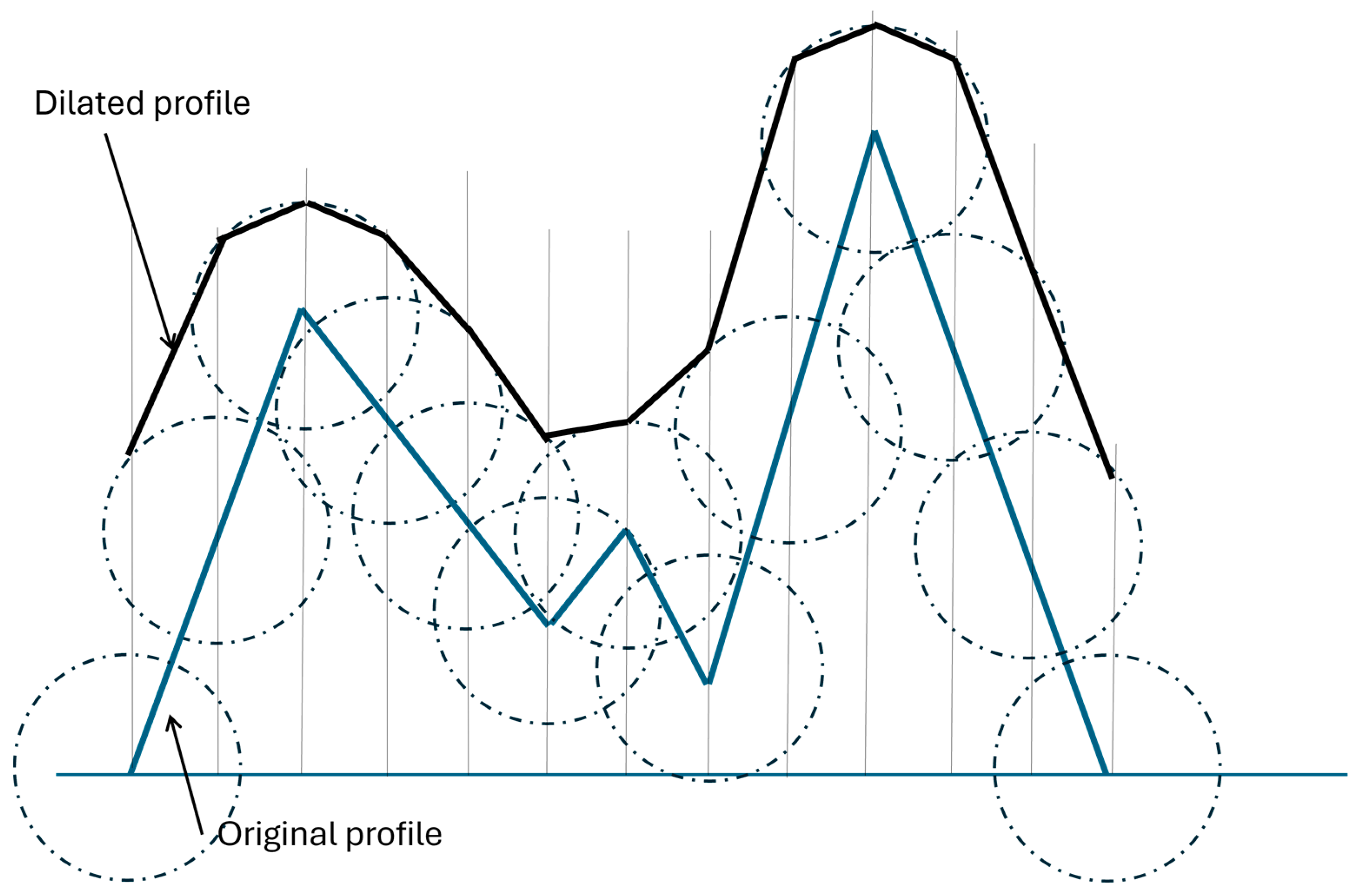
Figure 6.
Morphological dilation operation based on [
9].
Figure 6.
Morphological dilation operation based on [
9].
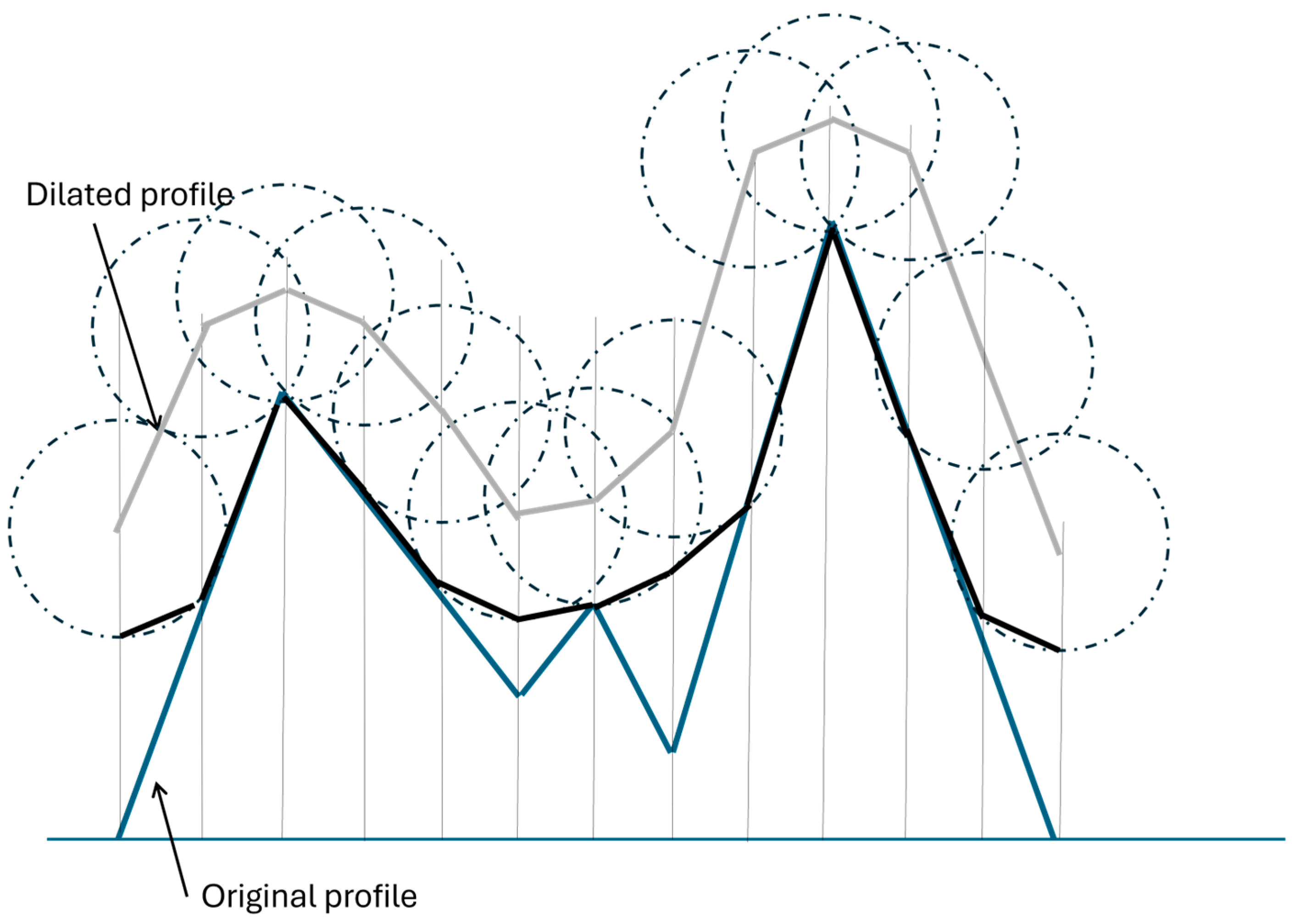
Figure 7.
Morphological closing operation based on [
9].
Figure 7.
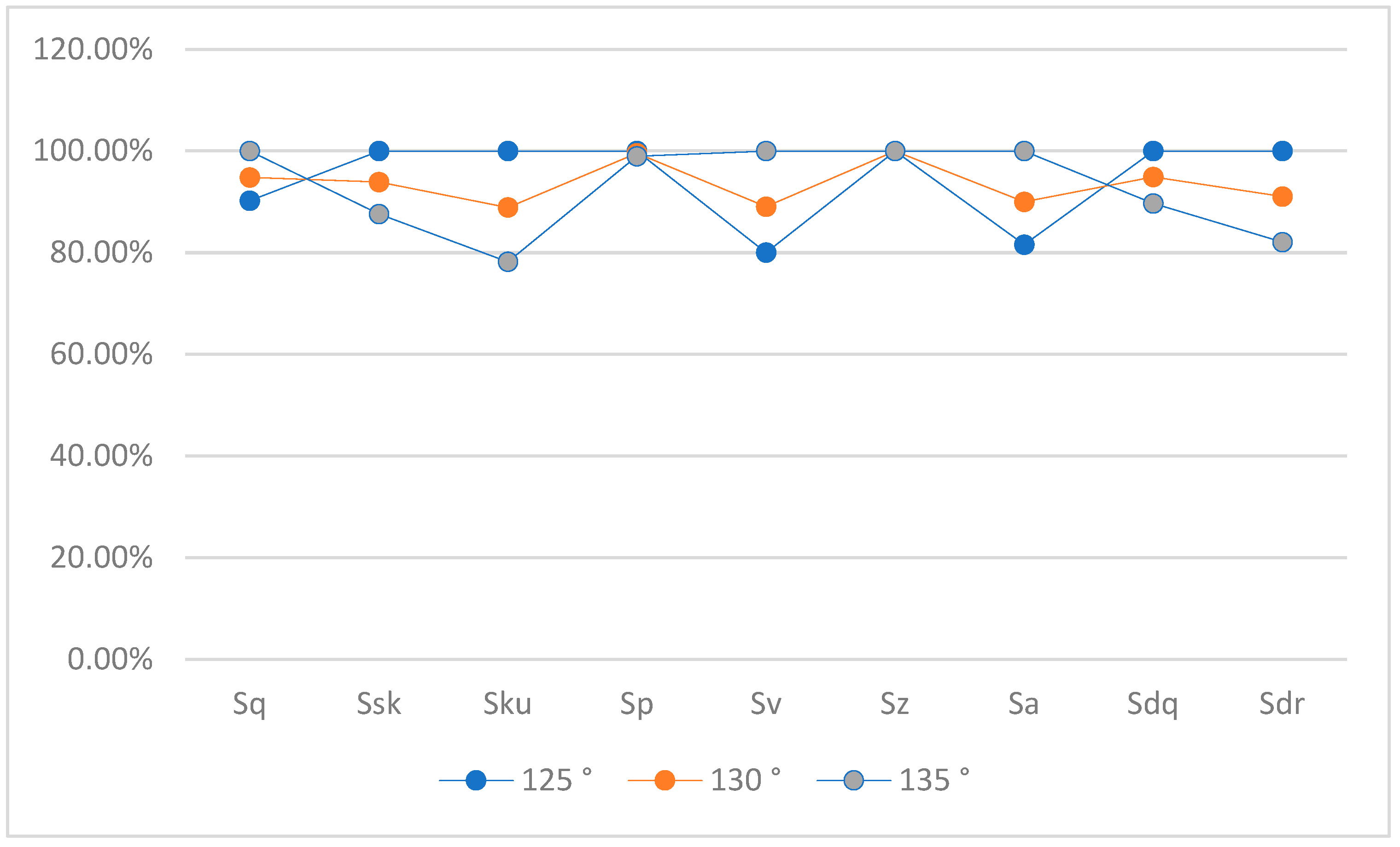
Morphological closing operation based on [
9].
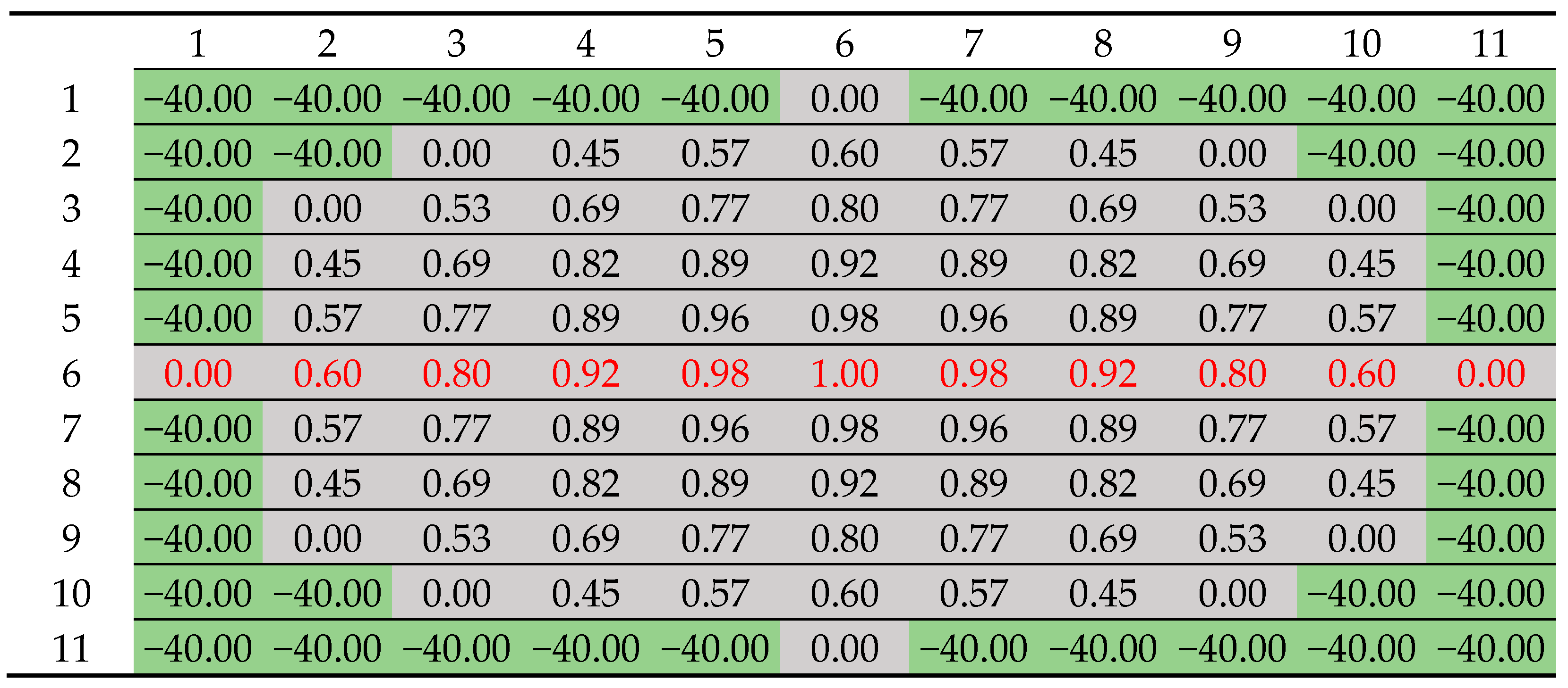
Figure 8.
FAMCB filter matrix for 2 µm stylus size (values in µm).
Figure 8.
FAMCB filter matrix for 2 µm stylus size (values in µm).
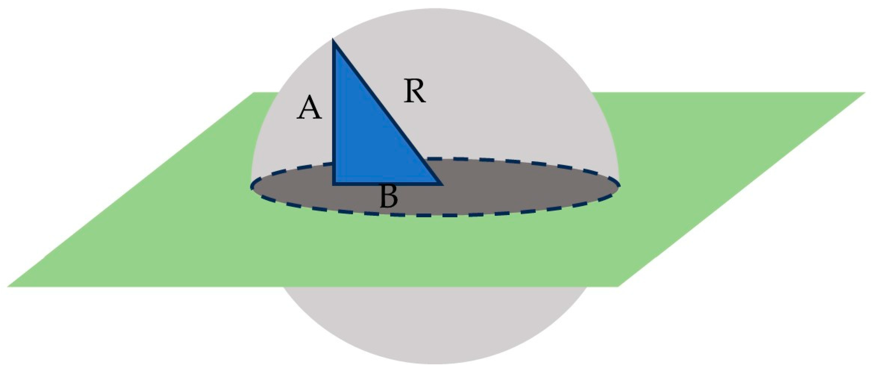
Figure 9.
Sphere (particle) and diametric plane.
Figure 9.
Sphere (particle) and diametric plane.
Figure 10.
(a) Original point cloud discarding the points that, once filtered, are affected by the end effect. Z (height in µm), X, and Y (horizontal displacement in µm). (b) Point cloud resulting from filtering with the 70 µm filter. Z (height in µm), X, and Y (horizontal displacement in µm).
Figure 10.
(a) Original point cloud discarding the points that, once filtered, are affected by the end effect. Z (height in µm), X, and Y (horizontal displacement in µm). (b) Point cloud resulting from filtering with the 70 µm filter. Z (height in µm), X, and Y (horizontal displacement in µm).
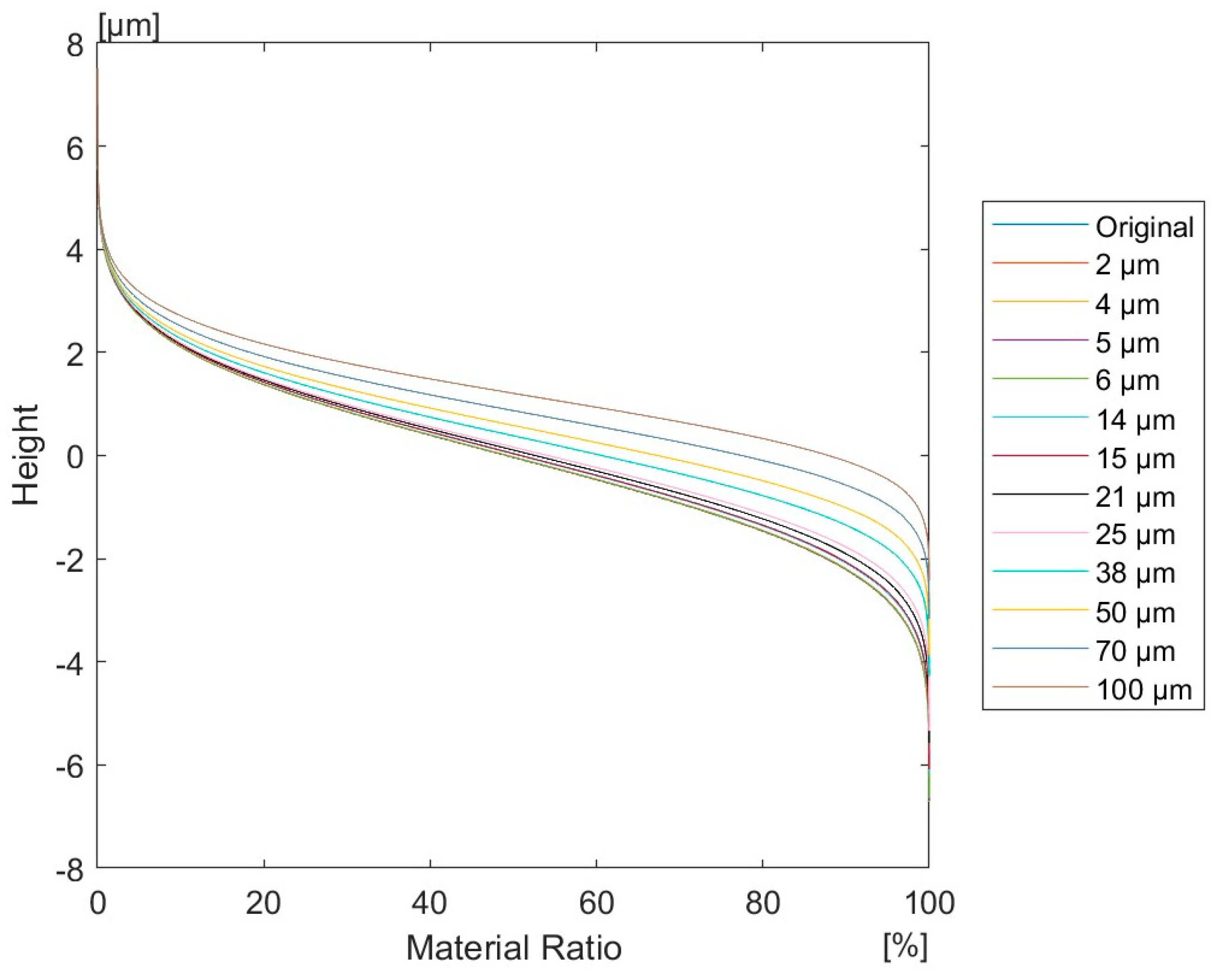
Figure 11.
Material ratio curves of the original and filtered point cloud with various filter sizes. Vertical axis (height in µm) and horizontal axis (Material ratio in %).
Figure 11.
Material ratio curves of the original and filtered point cloud with various filter sizes. Vertical axis (height in µm) and horizontal axis (Material ratio in %).
Figure 12.
Graph of the variation in results between original and filtered point clouds.
Figure 12.
Graph of the variation in results between original and filtered point clouds.
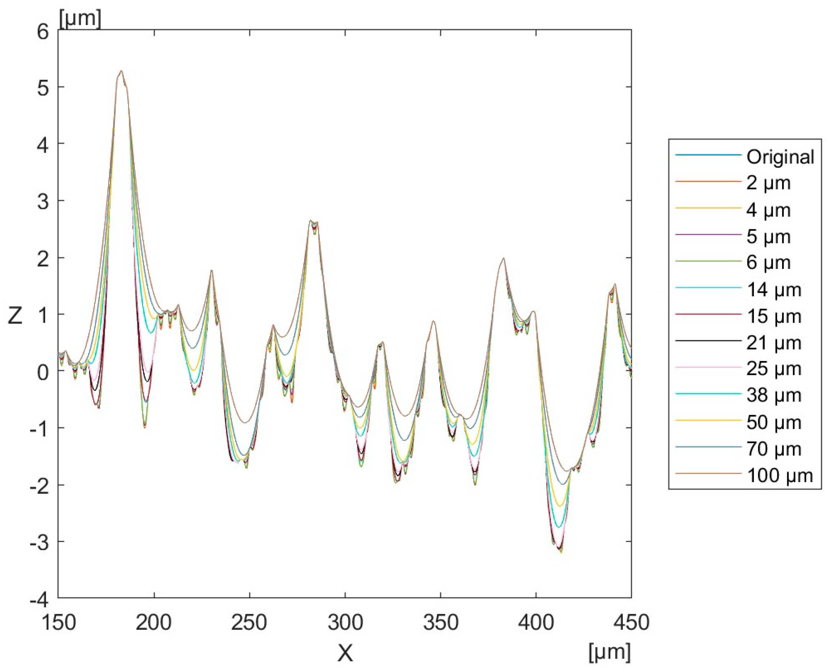
Figure 13.
Original profile and filtered profile with different sizes. Z (height in µm) and X (horizontal displacement in µm).
Figure 13.
Original profile and filtered profile with different sizes. Z (height in µm) and X (horizontal displacement in µm).
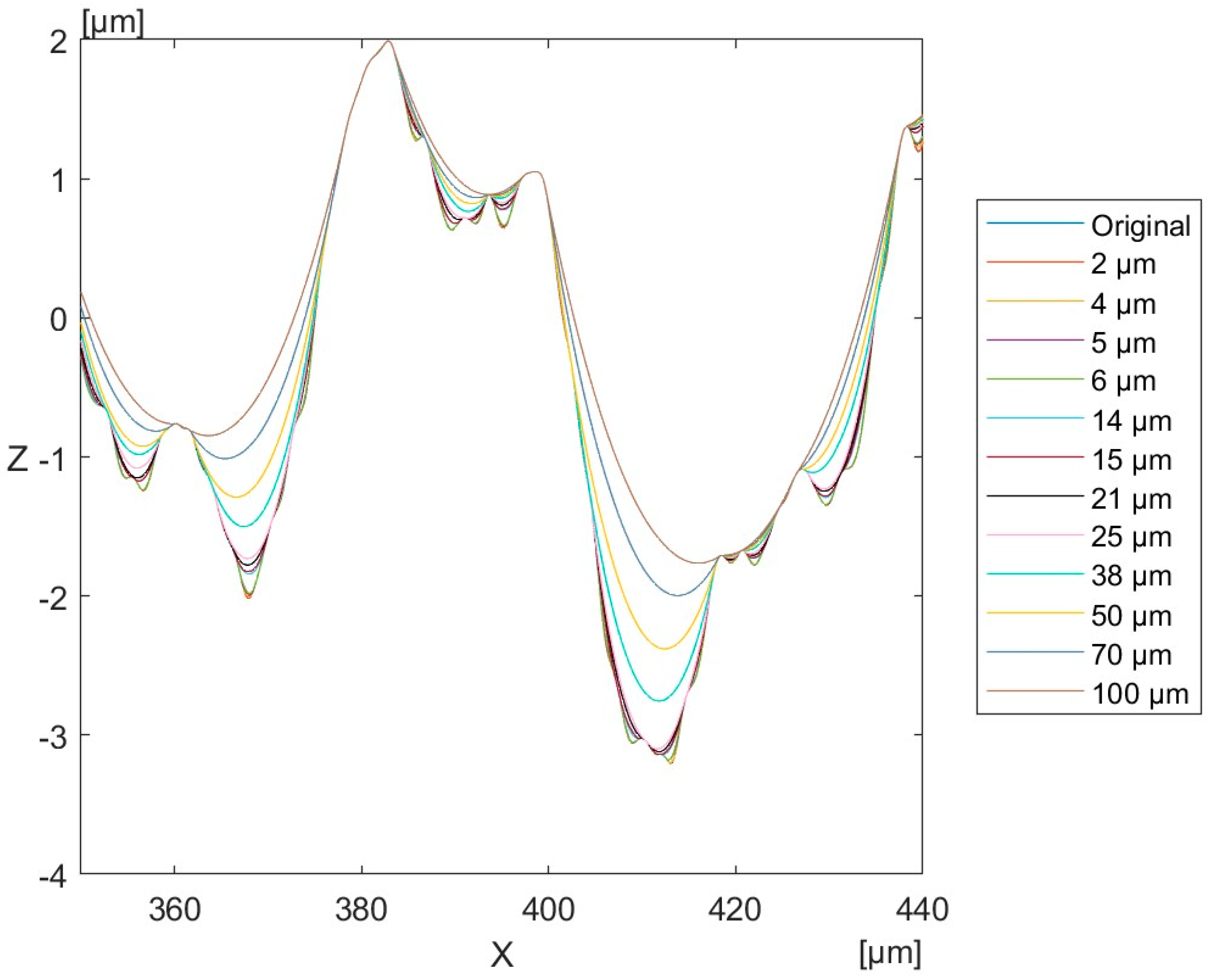
Figure 14.
Original and filtered profiles expanded. Z (height in µm) and X (horizontal displacement in µm).
Figure 14.
Original and filtered profiles expanded. Z (height in µm) and X (horizontal displacement in µm).
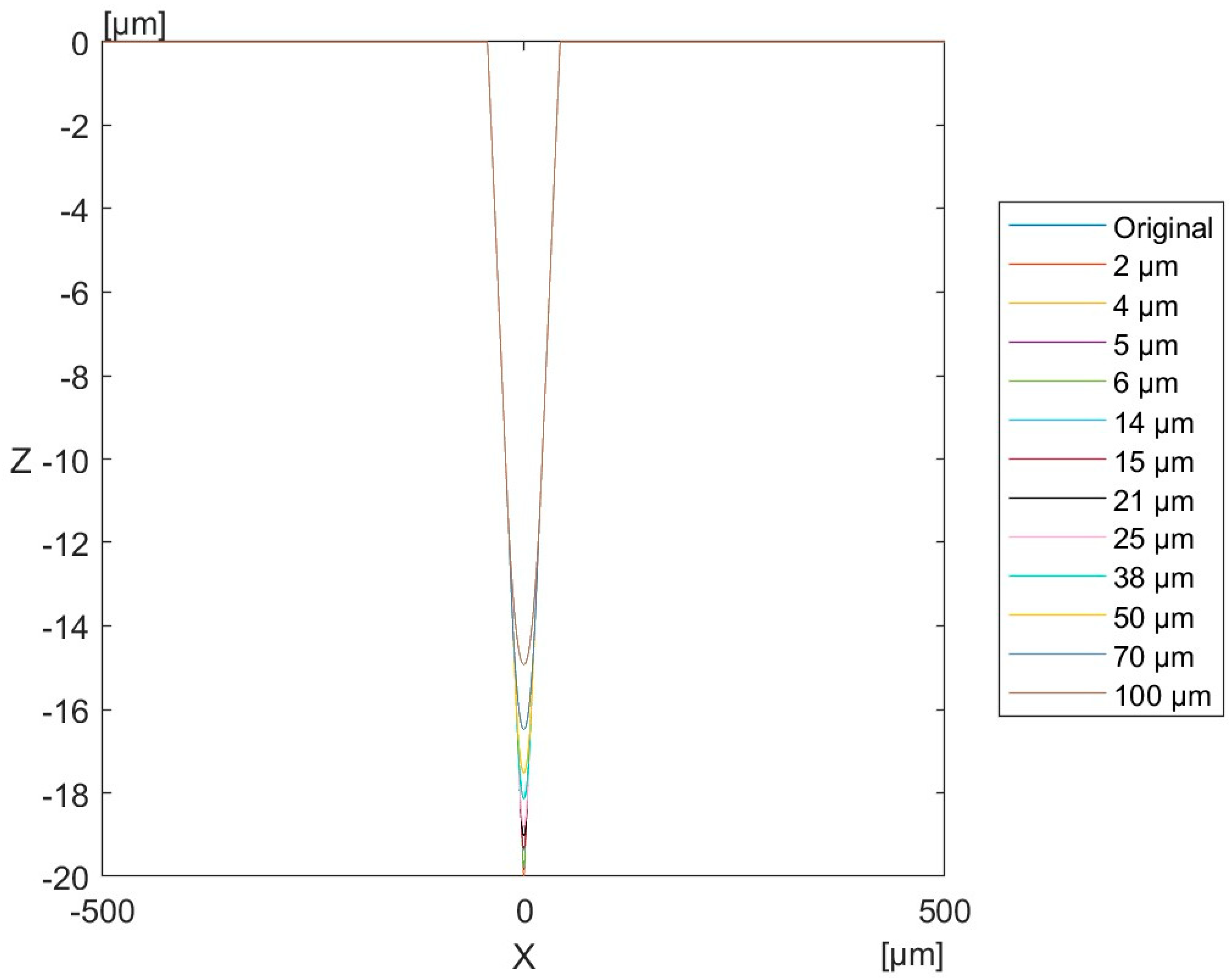
Figure 15.
Original and filtered profiles greatly expanded. Z (height in µm) and X (horizontal displacement in µm).
Figure 15.
Original and filtered profiles greatly expanded. Z (height in µm) and X (horizontal displacement in µm).
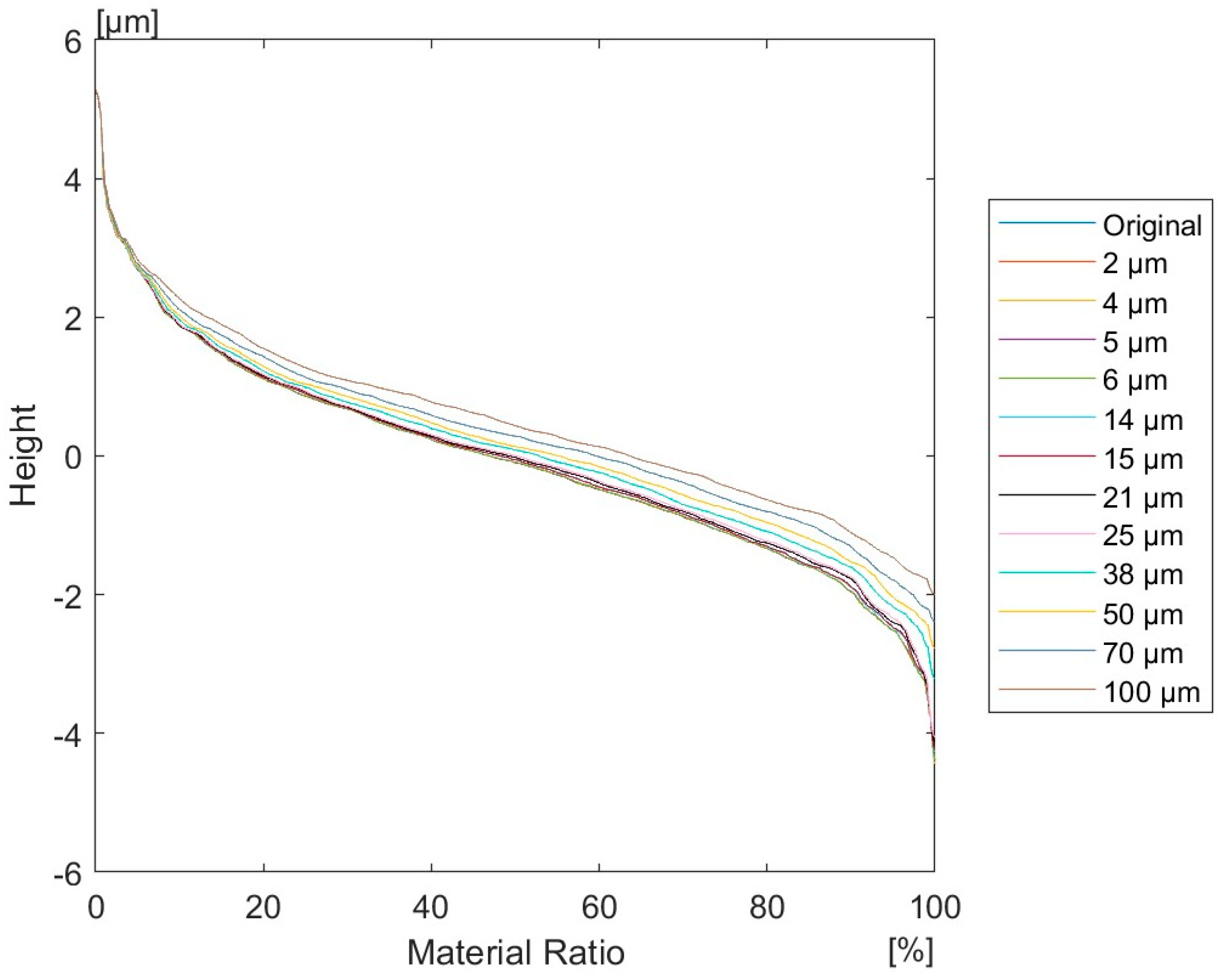
Figure 16.
Comparison of the material ratio curve of the original and filtered profiles. Vertical axis (height in µm) and horizontal axis (Material ratio in %).
Figure 16.
Comparison of the material ratio curve of the original and filtered profiles. Vertical axis (height in µm) and horizontal axis (Material ratio in %).
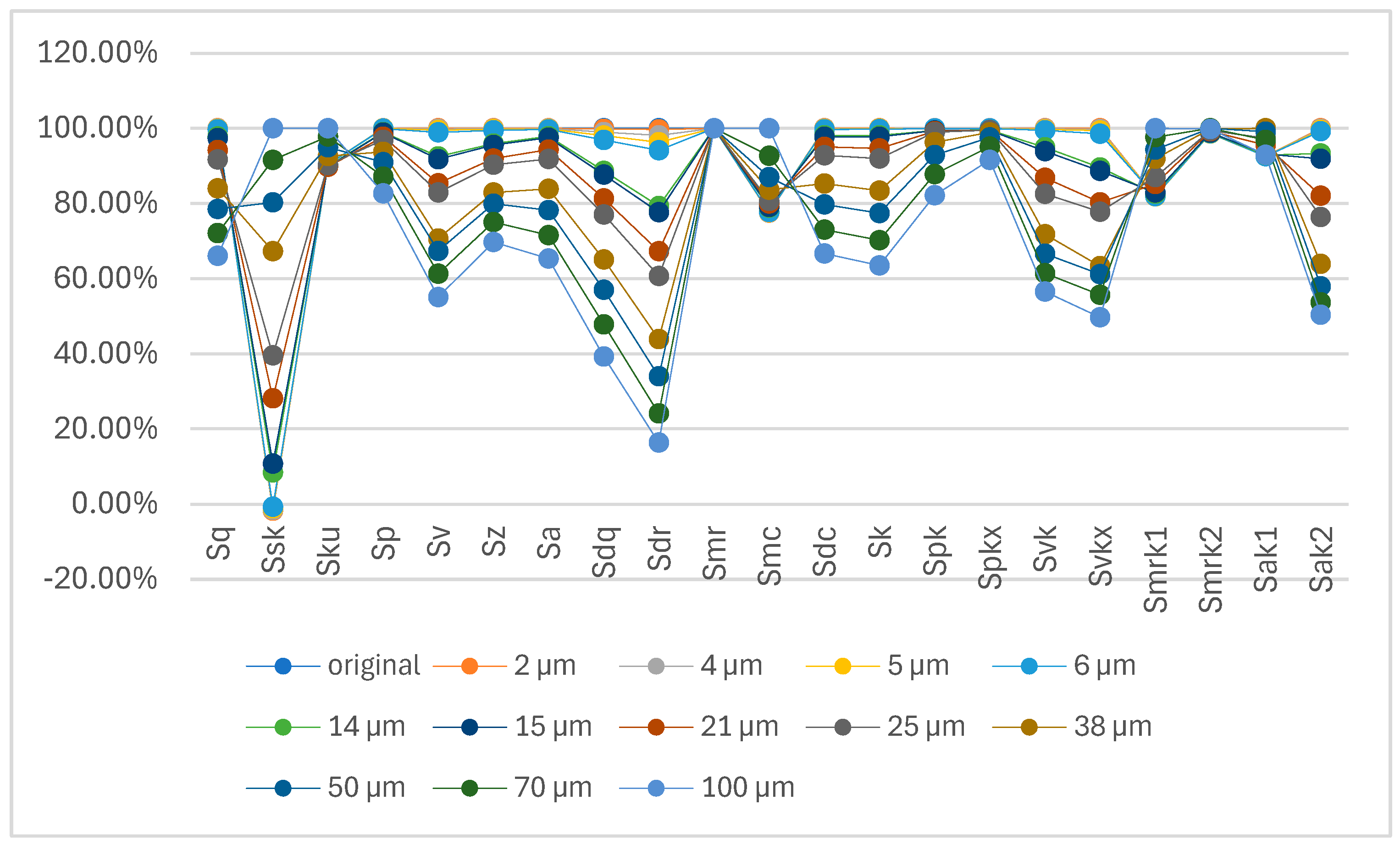
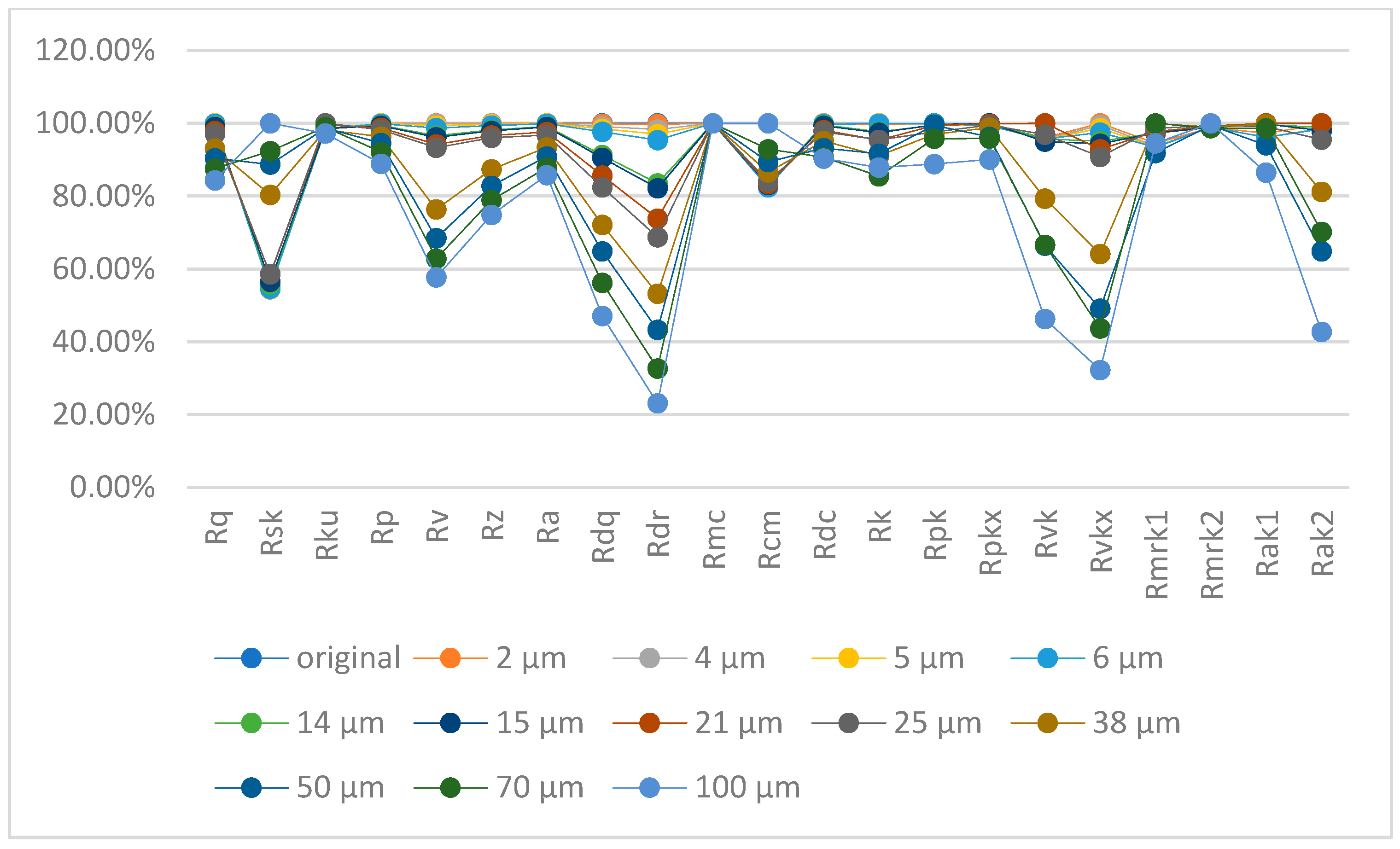
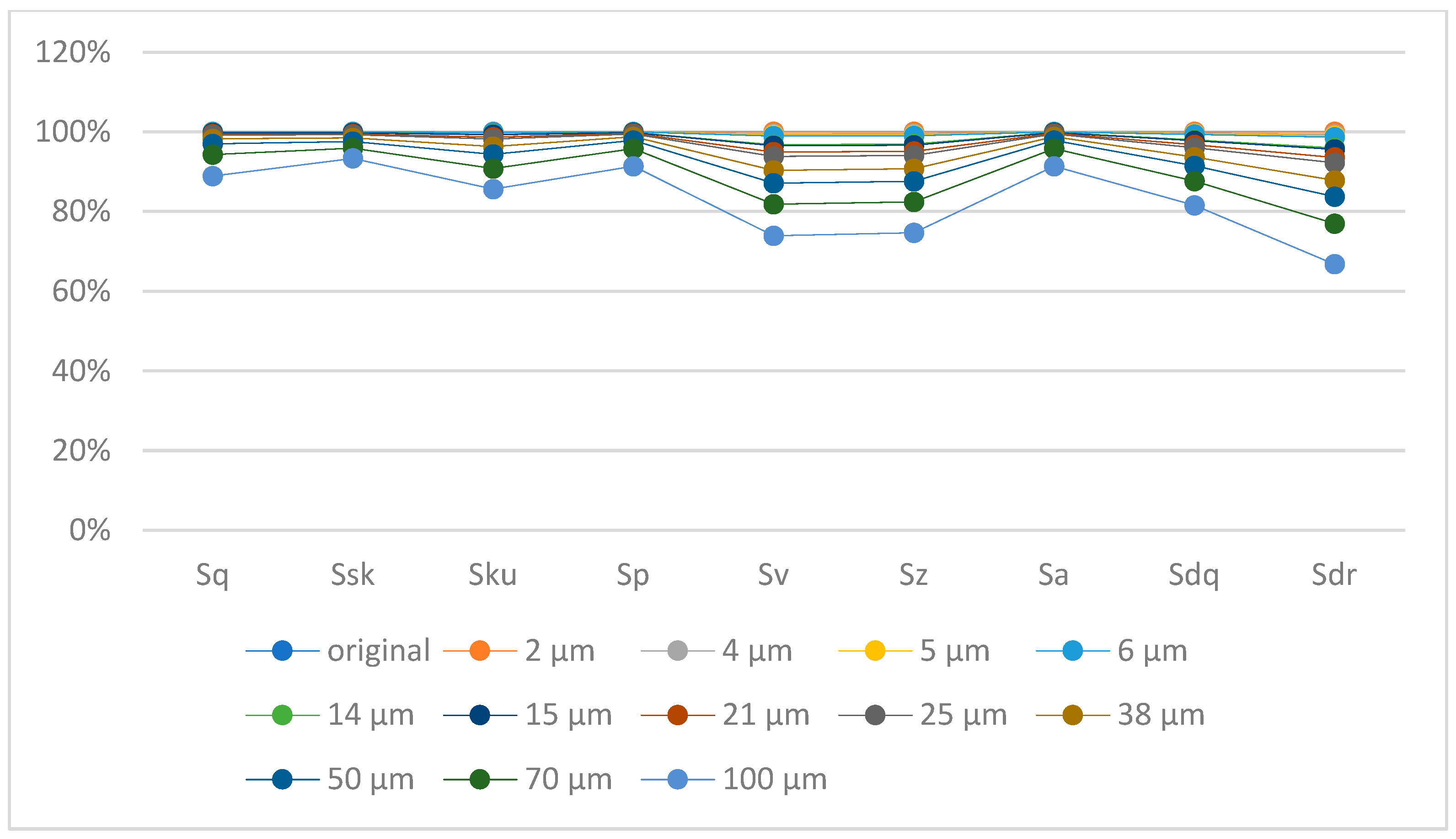
Figure 17.
Graphical representation of the evolution of the areal roughness parameters in the surface for each analysed filter.
Figure 17.
Graphical representation of the evolution of the areal roughness parameters in the surface for each analysed filter.
Figure 18.
Graphical comparison of the shape of the original and filtered groove standard. Z (height in µm) and X (horizontal displacement in µm).
Figure 18.
Graphical comparison of the shape of the original and filtered groove standard. Z (height in µm) and X (horizontal displacement in µm).
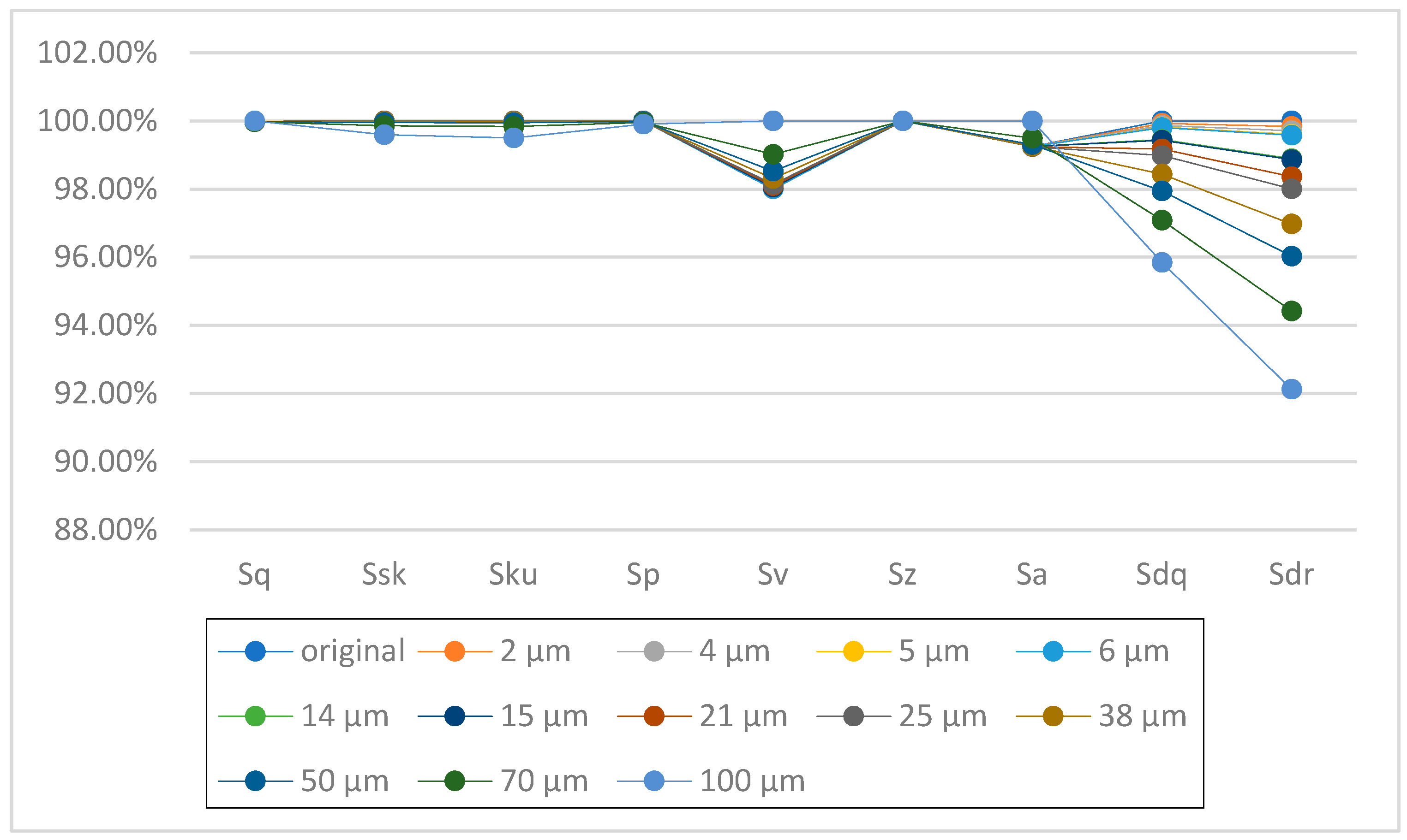
Figure 19.
Graphical representation of the evolution of the areal roughness parameters in the groove standard for each analysed filter.
Figure 19.
Graphical representation of the evolution of the areal roughness parameters in the groove standard for each analysed filter.
Figure 20.
Graphical comparison of the shape of the original and filtered peak standard. Z (height in µm) and X (horizontal displacement in µm).
Figure 20.
Graphical comparison of the shape of the original and filtered peak standard. Z (height in µm) and X (horizontal displacement in µm).
Figure 21.
The original and filtered peak standard expanded. Z (height in µm) and X (horizontal displacement in µm).
Figure 21.
The original and filtered peak standard expanded. Z (height in µm) and X (horizontal displacement in µm).
Figure 22.
Graphical representation of the evolution of the areal roughness parameters in the peak standard for each analysed filter.
Figure 22.
Graphical representation of the evolution of the areal roughness parameters in the peak standard for each analysed filter.
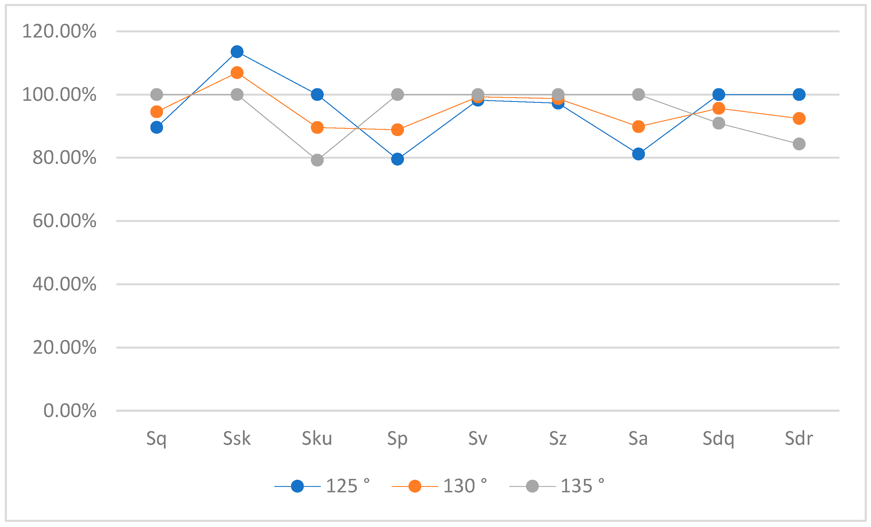
Figure 23.
Graphical comparison of applying a 5 µm filter and a ±5° alpha variation in a groove standard.
Figure 23.
Graphical comparison of applying a 5 µm filter and a ±5° alpha variation in a groove standard.
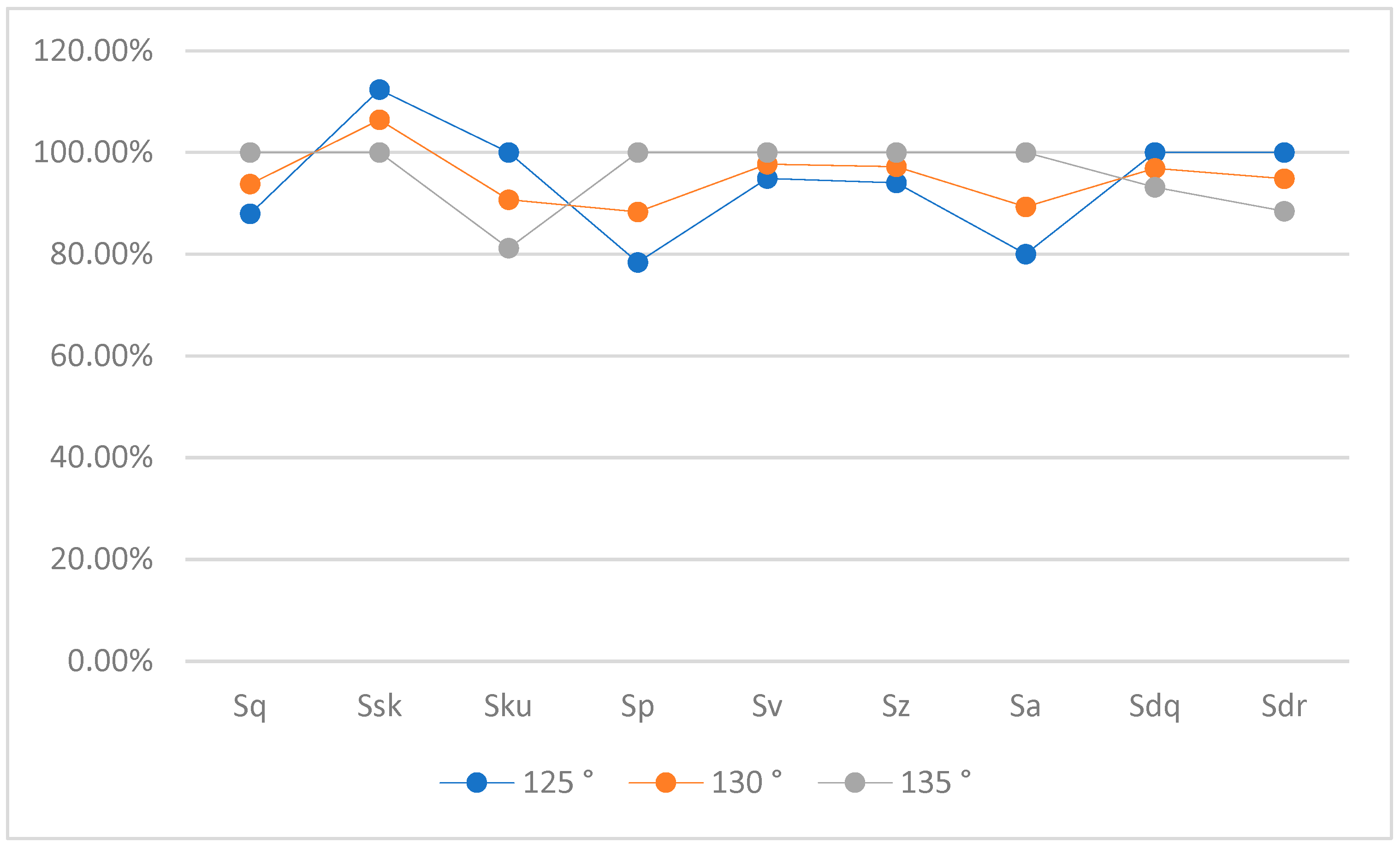
Figure 24.
Graphical comparison of applying a 25 µm filter and a ±5° alpha variation in a groove standard.
Figure 24.
Graphical comparison of applying a 25 µm filter and a ±5° alpha variation in a groove standard.
Figure 25.
Graphical comparison of applying a 50 µm filter and a ±5° alpha variation in a groove standard.
Figure 25.
Graphical comparison of applying a 50 µm filter and a ±5° alpha variation in a groove standard.
Figure 26.
Graphical comparison of applying a 100 µm filter and a ±5° alpha variation in a groove standard.
Figure 26.
Graphical comparison of applying a 100 µm filter and a ±5° alpha variation in a groove standard.
Figure 27.
Graphical comparison of applying a 5 µm filter and a ±5° alpha variation in a peak standard.
Figure 27.
Graphical comparison of applying a 5 µm filter and a ±5° alpha variation in a peak standard.
Figure 28.
Graphical comparison of applying a 25 µm filter and a ±5° alpha variation in a peak standard.
Figure 28.
Graphical comparison of applying a 25 µm filter and a ±5° alpha variation in a peak standard.
Figure 29.
Graphical comparison of applying a 50 µm filter and a ±5° alpha variation in a peak standard.
Figure 29.
Graphical comparison of applying a 50 µm filter and a ±5° alpha variation in a peak standard.
Figure 30.
Graphical comparison of applying a 100 µm filter and a ±5° alpha variation in a peak standard.
Figure 30.
Graphical comparison of applying a 100 µm filter and a ±5° alpha variation in a peak standard.
Figure 31.
Graphical representation of the variation in results of applying a ±5% stylus size variation to the 5 µm stylus for the groove standard with α = 130°.
Figure 31.
Graphical representation of the variation in results of applying a ±5% stylus size variation to the 5 µm stylus for the groove standard with α = 130°.
Figure 32.
Graphical representation of the variation in results of applying a ±5% stylus size variation to the 25 µm stylus for the groove standard with α = 130°.
Figure 32.
Graphical representation of the variation in results of applying a ±5% stylus size variation to the 25 µm stylus for the groove standard with α = 130°.
Figure 33.
Graphical representation of the variation in results of applying a ±5% stylus size variation to the 50 µm stylus for the groove standard with α = 130°.
Figure 33.
Graphical representation of the variation in results of applying a ±5% stylus size variation to the 50 µm stylus for the groove standard with α = 130°.
Figure 34.
Graphical representation of the variation in results of applying a ±5% stylus size variation to the 100 µm stylus for the groove standard with α = 130°.
Figure 34.
Graphical representation of the variation in results of applying a ±5% stylus size variation to the 100 µm stylus for the groove standard with α = 130°.
Figure 35.
Graphical representation of the variation in results of applying a ±5% stylus size variation to the 5 µm stylus for the peak standard with α = 130°.
Figure 35.
Graphical representation of the variation in results of applying a ±5% stylus size variation to the 5 µm stylus for the peak standard with α = 130°.
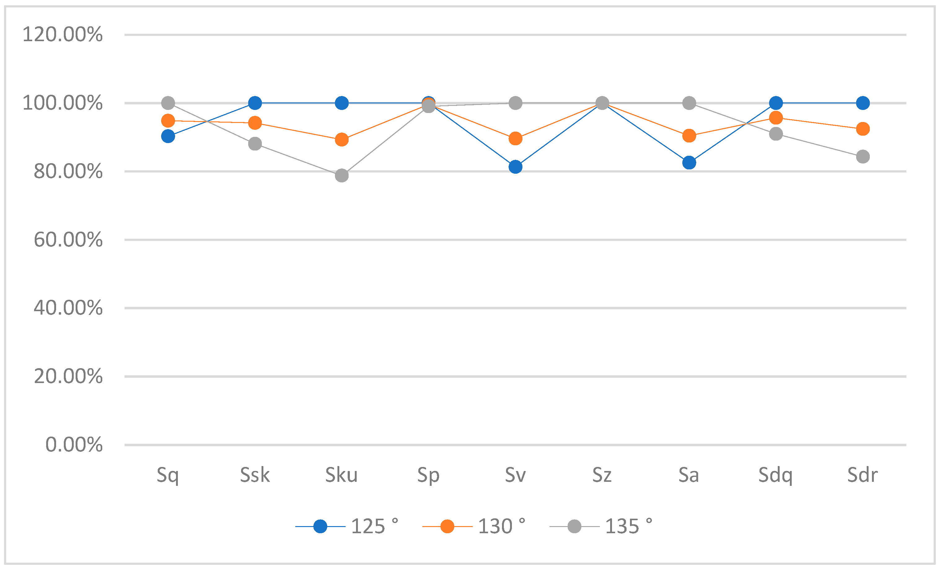
Figure 36.
Graphical representation of the variation in results of applying a ±5% stylus size variation to the 25 µm stylus for the peak standard with α = 130°.
Figure 36.
Graphical representation of the variation in results of applying a ±5% stylus size variation to the 25 µm stylus for the peak standard with α = 130°.
Figure 37.
Graphical representation of the variation in results of applying a ±5% stylus size variation to the 50 µm stylus for the peak standard with α = 130°.
Figure 37.
Graphical representation of the variation in results of applying a ±5% stylus size variation to the 50 µm stylus for the peak standard with α = 130°.
Figure 38.
Graphical representation of the variation in results of applying a ±5% stylus size variation to the 100 µm stylus for the peak standard with α = 130°.
Figure 38.
Graphical representation of the variation in results of applying a ±5% stylus size variation to the 100 µm stylus for the peak standard with α = 130°.
Table 1.
Table of particle sizes for each of the standards.
Table 1.
Table of particle sizes for each of the standards.
| Standards with Particle Sizes | Standards with Calibration Procedures | Size [µm] |
|---|
| ISO 4406:2021 [14] | ISO 4407:2002 [21] | 4, 6, 14 |
| ISO 11171:2022 [22] | 5, 15 |
| NAS 1638:1964 [15,16,17]; | ISO 4402:1977 [23] | [5–15], [15–25], [25–50], [50–100] |
| SAE AS4059 Rev. E [16,17,18] | ISO 4402:1991 [24,25] | 4, 6, 14, 21, 38, 70 |
| ISO 11171:2022 [22] | 2, 5, 15, 25, 50, 100 |
| GOST 17216:2001 [16,17,19]; | ISO 4402:1991 [24,25] | [5–10], [10–25], [25–50], [50–100], [100–200] |
| NAV AIR 10-1A17 (1989) [16,17,20] | - | [5–10], [10–25], [25–50], [50–100], >100 |
Table 2.
Parameters evaluated.
Table 2.
Parameters evaluated.
| Type of Parameters | Surface Parameters | Profile Parameters |
|---|
| Height parameters | ) | ) |
| ) | ) |
| ) | ) |
| *) | *) |
| *) | *) |
| *) | *) |
| ) | ) |
| Hybrid parameters | ) | ) |
| ) | ) |
| Material ratio parameters and functions | ) | ) |
| ) | ) |
| ) | ) |
| Areal parameters for stratified surfaces | ) | ) |
| ) | ) |
| ) | ) |
| ) | ) |
| ) | ) |
| ) | ) |
| ) | ) |
| ) | ) |
| ) | ) |
Table 3.
Results of the surface roughness of the original and filtered clouds (2–15 µm).
Table 3.
Results of the surface roughness of the original and filtered clouds (2–15 µm).
| Parameters | Original | 2 µm | 4 µm | 5 µm | 6 µm | 14 µm | 15 µm |
|---|
| [µm] | 1.6825 | 1.6823 | 1.6811 | 1.6795 | 1.6773 | 1.6452 | 1.6385 |
| −0.0056 | −0.0055 | −0.0046 | −0.0036 | −0.0023 | 0.0261 | 0.0334 |
| 2.9573 | 2.9572 | 2.9568 | 2.9564 | 2.9560 | 2.9402 | 2.9375 |
| [µm] | 7.5584 | 7.5577 | 7.5551 | 7.5514 | 7.5462 | 7.4800 | 7.4691 |
| [µm] | 6.6769 | 6.6776 | 6.6641 | 6.6455 | 6.6051 | 6.1742 | 6.1270 |
| [µm] | 14.2354 | 14.2354 | 14.2191 | 14.1969 | 14.1514 | 13.6542 | 13.5960 |
| [µm] | 1.3458 | 1.3456 | 1.3447 | 1.3434 | 1.3417 | 1.3171 | 1.3119 |
| [rad] | 0.4304 | 0.4295 | 0.4259 | 0.4218 | 0.4170 | 0.3814 | 0.3772 |
| [%] | 8.6407 | 8.6148 | 8.4735 | 8.3158 | 8.1333 | 6.8526 | 6.7066 |
| [%] | 10.0000 | 10.0000 | 10.0000 | 10.0000 | 10.0000 | 10.0000 | 10.0000 |
| [µm] | 2.1002 | 2.1006 | 2.1018 | 2.1036 | 2.1061 | 2.1372 | 2.1413 |
| [µm] | 3.5727 | 3.5722 | 3.5697 | 3.5665 | 3.5622 | 3.5037 | 3.4922 |
| [µm] | 4.3760 | 4.3755 | 4.3727 | 4.3689 | 4.3639 | 4.2916 | 4.2757 |
| [µm] | 1.5694 | 1.5692 | 1.5690 | 1.5685 | 1.5677 | 1.5596 | 1.5591 |
| [µm] | 5.3631 | 5.3627 | 5.3617 | 5.3602 | 5.3580 | 5.3351 | 5.3344 |
| [µm] | 1.5673 | 1.5669 | 1.5647 | 1.5619 | 1.5580 | 1.4876 | 1.4717 |
| [µm] | 4.4962 | 4.4972 | 4.4847 | 4.4677 | 4.4294 | 4.0275 | 3.9859 |
| [%] | 9.5198 | 9.5202 | 9.5227 | 9.5253 | 9.5293 | 9.6107 | 9.6445 |
| [%] | 90.0966 | 90.0973 | 90.1033 | 90.1090 | 90.1169 | 90.2672 | 90.3132 |
| [µm3/mm2] | 74.7000 | 74.6978 | 74.7041 | 74.6999 | 74.6941 | 74.9462 | 75.1860 |
| [µm3/mm2] | 77.6061 | 77.5852 | 77.4290 | 77.2451 | 76.9882 | 72.3932 | 71.2780 |
Table 4.
Results of the surface roughness parameters of the filtered clouds (21–100 µm).
Table 4.
Results of the surface roughness parameters of the filtered clouds (21–100 µm).
| Parameters | 21 µm | 25 µm | 38 µm | 50 µm | 70 µm | 100 µm |
|---|
| [µm] | 1.5848 | 1.5426 | 1.4127 | 1.3209 | 1.2125 | 1.1109 |
| 0.0873 | 0.1227 | 0.2088 | 0.2491 | 0.2841 | 0.3102 |
| 2.9364 | 2.9522 | 3.0300 | 3.1063 | 3.2002 | 3.2732 |
| [µm] | 7.3869 | 7.3200 | 7.0813 | 6.8738 | 6.5819 | 6.2478 |
| [µm] | 5.6975 | 5.5356 | 4.7164 | 4.4972 | 4.0934 | 3.6758 |
| [µm] | 13.0845 | 12.8556 | 11.7977 | 11.3709 | 10.6753 | 9.9236 |
| [µm] | 1.2695 | 1.2353 | 1.1284 | 1.0526 | 0.9629 | 0.8794 |
| [rad] | 0.3498 | 0.3315 | 0.2800 | 0.2453 | 0.2057 | 0.1690 |
| [%] | 5.8130 | 5.2451 | 3.7930 | 2.9366 | 2.0815 | 1.4130 |
| [%] | 10.0000 | 10.0000 | 10.0000 | 10.0000 | 10.0000 | 10.0000 |
| [µm] | 2.1660 | 2.1850 | 2.2663 | 2.3573 | 2.5106 | 2.7095 |
| [µm] | 3.3961 | 3.3148 | 3.0459 | 2.8475 | 2.6087 | 2.3816 |
| [µm] | 4.1399 | 4.0225 | 3.6501 | 3.3878 | 3.0714 | 2.7794 |
| [µm] | 1.5568 | 1.5528 | 1.5110 | 1.4573 | 1.3774 | 1.2890 |
| [µm] | 5.3351 | 5.3362 | 5.3020 | 5.2312 | 5.1007 | 4.9107 |
| [µm] | 1.3599 | 1.2932 | 1.1251 | 1.0439 | 0.9626 | 0.8856 |
| [µm] | 3.6095 | 3.4969 | 2.8456 | 2.7519 | 2.5032 | 2.2335 |
| [%] | 9.9076 | 10.1207 | 10.6837 | 10.9739 | 11.3506 | 11.6327 |
| [%] | 90.6360 | 90.8333 | 91.1788 | 91.3833 | 91.3464 | 91.1754 |
| [µm3/mm2] | 77.1222 | 78.5763 | 80.7170 | 79.9638 | 78.1706 | 74.9701 |
| [µm3/mm2] | 63.6721 | 59.2715 | 49.6228 | 44.9760 | 41.6490 | 39.0753 |
Table 5.
Results of the profile roughness of the original and filtered clouds (2–15 µm).
Table 5.
Results of the profile roughness of the original and filtered clouds (2–15 µm).
| Parameters | Original | 2 µm | 4 µm | 5 µm | 6 µm | 14 µm | 15 µm |
|---|
| [µm] | 1.5478 | 1.5477 | 1.5474 | 1.5469 | 1.5460 | 1.5349 | 1.5320 |
| 0.2952 | 0.2952 | 0.2949 | 0.2951 | 0.2957 | 0.3023 | 0.3061 |
| 3.4020 | 3.4019 | 3.4014 | 3.4002 | 3.3986 | 3.4001 | 3.4026 |
| [µm] | 5.3538 | 5.3535 | 5.3521 | 5.3506 | 5.3485 | 5.3216 | 5.3172 |
| [µm] | 4.3783 | 4.3787 | 4.3742 | 4.3515 | 4.3204 | 4.2297 | 4.2092 |
| [µm] | 9.7321 | 9.7321 | 9.7264 | 9.7022 | 9.6689 | 9.5512 | 9.5264 |
| [µm] | 1.2068 | 1.2067 | 1.2064 | 1.2060 | 1.2053 | 1.1963 | 1.1943 |
| [rad] | 0.2986 | 0.2981 | 0.2960 | 0.2940 | 0.2915 | 0.2726 | 0.2703 |
| [%] | 4.2369 | 4.2268 | 4.1656 | 4.1101 | 4.0412 | 3.5374 | 3.4805 |
| [%] | 10.0000 | 10.0000 | 10.0000 | 10.0000 | 10.0000 | 10.0000 | 10.0000 |
| [µm] | 1.8687 | 1.8687 | 1.8711 | 1.8687 | 1.8687 | 1.8841 | 1.8826 |
| [µm] | 3.2085 | 3.2085 | 3.2090 | 3.2051 | 3.2027 | 3.1947 | 3.1871 |
| [µm] | 3.7311 | 3.7306 | 3.7479 | 3.7461 | 3.7425 | 3.6595 | 3.6510 |
| [µm] | 1.8802 | 1.8794 | 1.8743 | 1.8772 | 1.8788 | 1.8690 | 1.8717 |
| [µm] | 3.5332 | 3.5331 | 3.5218 | 3.5211 | 3.5204 | 3.5450 | 3.5460 |
| [µm] | 1.4236 | 1.4230 | 1.4160 | 1.4161 | 1.4192 | 1.4188 | 1.4083 |
| [µm] | 2.4678 | 2.4684 | 2.4566 | 2.4349 | 2.4060 | 2.3467 | 2.3295 |
| [%] | 11.8097 | 11.8149 | 11.7124 | 11.6901 | 11.6812 | 12.1646 | 12.1694 |
| [%] | 90.1687 | 90.1639 | 90.2265 | 90.2338 | 90.2566 | 90.2128 | 90.2299 |
| [µm2/mm] | 111.0213 | 111.0229 | 109.7636 | 109.7209 | 109.7343 | 113.6792 | 113.8854 |
| [µm2/mm] | 69.9784 | 69.9824 | 69.1953 | 69.1502 | 69.1399 | 69.4281 | 68.7978 |
Table 6.
Results of the profile roughness parameters of the filtered clouds (21–100 µm).
Table 6.
Results of the profile roughness parameters of the filtered clouds (21–100 µm).
| Parameters | 21 µm | 25 µm | 38 µm | 50 µm | 70 µm | 100 µm |
|---|
| [µm] | 1.5141 | 1.5029 | 1.4405 | 1.3987 | 1.3546 | 1.3046 |
| 0.3169 | 0.3174 | 0.4353 | 0.4805 | 0.5002 | 0.5417 |
| 3.4372 | 3.4523 | 3.3889 | 3.4063 | 3.4154 | 3.3557 |
| [µm] | 5.2845 | 5.2592 | 5.1560 | 5.0634 | 4.9296 | 4.7585 |
| [µm] | 4.1236 | 4.0864 | 3.3434 | 2.9977 | 2.7497 | 2.5255 |
| [µm] | 9.4081 | 9.3456 | 8.4994 | 8.0611 | 7.6793 | 7.2840 |
| [µm] | 1.1780 | 1.1680 | 1.1270 | 1.0966 | 1.0601 | 1.0350 |
| [rad] | 0.2556 | 0.2462 | 0.2154 | 0.1936 | 0.1677 | 0.1406 |
| [%] | 3.1284 | 2.9103 | 2.2543 | 1.8329 | 1.3845 | 0.9790 |
| [%] | 10.0000 | 10.0000 | 10.0000 | 10.0000 | 10.0000 | 10.0000 |
| [µm] | 1.8904 | 1.9053 | 1.9619 | 2.0264 | 2.1060 | 2.2676 |
| [µm] | 3.1473 | 3.1347 | 3.0525 | 2.9907 | 2.9098 | 2.8986 |
| [µm] | 3.5738 | 3.5772 | 3.4146 | 3.4346 | 3.2031 | 3.2932 |
| [µm] | 1.8679 | 1.8349 | 1.8230 | 1.8694 | 1.8005 | 1.6701 |
| [µm] | 3.5418 | 3.5276 | 3.5023 | 3.4137 | 3.3975 | 3.1945 |
| [µm] | 1.4826 | 1.4364 | 1.1759 | 0.9848 | 0.9873 | 0.6862 |
| [µm] | 2.2925 | 2.2409 | 1.5825 | 1.2128 | 1.0787 | 0.7963 |
| [%] | 12.2189 | 12.3297 | 12.4866 | 11.4784 | 12.5013 | 11.8171 |
| [%] | 90.5259 | 90.6584 | 90.3033 | 90.7477 | 90.0200 | 91.2505 |
| [µm2/mm] | 114.1195 | 113.1207 | 113.8143 | 107.2857 | 112.5437 | 98.6763 |
| [µm2/mm] | 70.2334 | 67.0920 | 57.0128 | 45.5567 | 49.2659 | 30.0181 |
Table 7.
Results of the areal roughness parameters of the original and filtered groove standard (2–15 µm).
Table 7.
Results of the areal roughness parameters of the original and filtered groove standard (2–15 µm).
| Parameters | Original | 2 µm | 4 µm | 5 µm | 6 µm | 14 µm | 15 µm |
|---|
| Sq [µm] | 3.2957 | 3.2957 | 3.2951 | 3.2948 | 3.2943 | 3.2875 | 3.2863 |
| Ssk | −4.0838 | −4.0838 | −4.0831 | −4.0826 | −4.0819 | −4.0733 | −4.0718 |
| Sku | 19.1490 | 19.1490 | 19.1406 | 19.1344 | 19.1270 | 19.0269 | 19.0100 |
| Sp [µm] | 0.8665 | 0.8665 | 0.8664 | 0.8663 | 0.8663 | 0.8651 | 0.8648 |
| Sv [µm] | 19.1335 | 19.1335 | 19.0309 | 18.9794 | 18.9280 | 18.5148 | 18.4633 |
| Sz [µm] | 20.0000 | 20.0000 | 19.8973 | 19.8458 | 19.7943 | 19.3799 | 19.3281 |
| Sa [µm] | 1.5868 | 1.5868 | 1.5866 | 1.5865 | 1.5864 | 1.5842 | 1.5838 |
| Sdq [rad] | 0.1363 | 0.1363 | 0.1358 | 0.1356 | 0.1354 | 0.1335 | 0.1333 |
| Sdr [%] | 0.8842 | 0.8842 | 0.8784 | 0.8754 | 0.8724 | 0.8484 | 0.8454 |
Table 8.
Results of the areal roughness parameters of the filtered groove standard (21–100 µm).
Table 8.
Results of the areal roughness parameters of the filtered groove standard (21–100 µm).
| Parameters | 21 µm | 25 µm | 38 µm | 50 µm | 70 µm | 100 µm |
|---|
| Sq [µm] | 3.2773 | 3.2699 | 3.2372 | 3.1965 | 3.1077 | 2.9300 |
| Ssk | −4.0614 | −4.0531 | −4.0202 | −3.9841 | −3.9170 | −3.8120 |
| Sku | 18.8919 | 18.7994 | 18.4419 | 18.0627 | 17.3877 | 16.3956 |
| Sp [µm] | 0.8632 | 0.8618 | 0.8557 | 0.8478 | 0.8298 | 0.7916 |
| Sv [µm] | 18.1548 | 17.9497 | 17.2835 | 16.6712 | 15.6553 | 14.1429 |
| Sz [µm] | 19.0180 | 18.8115 | 18.1392 | 17.5190 | 16.4852 | 14.9345 |
| Sa [µm] | 1.5808 | 1.5783 | 1.5670 | 1.5525 | 1.5195 | 1.4494 |
| Sdq [rad] | 0.1318 | 0.1308 | 0.1276 | 0.1246 | 0.1194 | 0.1111 |
| Sdr [%] | 0.8274 | 0.8155 | 0.7765 | 0.7405 | 0.6806 | 0.5906 |
Table 9.
Results of the areal roughness parameters of the original and filtered peak standard (2–15 µm).
Table 9.
Results of the areal roughness parameters of the original and filtered peak standard (2–15 µm).
| Parameters | Original | 2 µm | 4 µm | 5 µm | 6 µm | 14 µm | 15 µm |
|---|
| Sq [µm] | 3.2957 | 3.2956 | 3.2956 | 3.2956 | 3.2956 | 3.2956 | 3.2956 |
| Ssk | 4.0838 | 4.0838 | 4.0838 | 4.0838 | 4.0838 | 4.0838 | 4.0838 |
| Sku | 19.1490 | 19.1491 | 19.1491 | 19.1491 | 19.1491 | 19.1491 | 19.1491 |
| Sp [µm] | 19.1335 | 19.1335 | 19.1335 | 19.1334 | 19.1334 | 19.1331 | 19.1331 |
| Sv [µm] | 0.8665 | 0.8665 | 0.8665 | 0.8666 | 0.8666 | 0.8669 | 0.8669 |
| Sz [µm] | 20.0000 | 20.0000 | 20.0000 | 20.0000 | 20.0000 | 20.0000 | 20.0000 |
| Sa [µm] | 1.5868 | 1.5868 | 1.5868 | 1.5868 | 1.5868 | 1.5867 | 1.5867 |
| Sdq [rad] | 0.1363 | 0.1362 | 0.1361 | 0.1360 | 0.1360 | 0.1355 | 0.1355 |
| Sdr [%] | 0.8842 | 0.8828 | 0.8817 | 0.8808 | 0.8806 | 0.8745 | 0.8742 |
Table 10.
Results of the areal roughness parameters of the filtered peak standard (21–100 µm).
Table 10.
Results of the areal roughness parameters of the filtered peak standard (21–100 µm).
| Parameters | 21 µm | 25 µm | 38 µm | 50 µm | 70 µm | 100 µm |
|---|
| Sq [µm] | 3.2955 | 3.2954 | 3.2952 | 3.2951 | 3.2951 | 3.2960 |
| Ssk | 4.0837 | 4.0836 | 4.0829 | 4.0818 | 4.0780 | 4.0673 |
| Sku | 19.1488 | 19.1483 | 19.1450 | 19.1389 | 19.1174 | 19.0532 |
| Sp [µm] | 19.1327 | 19.1323 | 19.1308 | 19.1289 | 19.1245 | 19.1158 |
| Sv [µm] | 0.8673 | 0.8677 | 0.8692 | 0.8711 | 0.8755 | 0.8842 |
| Sz [µm] | 20.0000 | 20.0000 | 20.0000 | 20.0000 | 20.0000 | 20.0000 |
| Sa [µm] | 1.5867 | 1.5866 | 1.5869 | 1.5876 | 1.5906 | 1.5988 |
| Sdq [rad] | 0.1352 | 0.1349 | 0.1342 | 0.1335 | 0.1323 | 0.1306 |
| Sdr [%] | 0.8697 | 0.8666 | 0.8575 | 0.8491 | 0.8349 | 0.8146 |
Table 11.
Results of applying a 5 µm filter and a ±5° variation in α for a groove standard.
Table 11.
Results of applying a 5 µm filter and a ±5° variation in α for a groove standard.
| Parameters | α = 125° | α = 130° | α = 135° |
|---|
| Sq [µm] | 3.1345 | 3.2948 | 3.4757 |
| Ssk | −4.3480 | −4.0826 | −3.8094 |
| Sku | 21.5168 | 19.1344 | 16.8381 |
| Sp [µm] | 0.7778 | 0.8663 | 0.9733 |
| Sv [µm] | 19.0317 | 18.9794 | 18.9036 |
| Sz [µm] | 19.8095 | 19.8458 | 19.8769 |
| Sa [µm] | 1.4377 | 1.5865 | 1.7625 |
| Sdq [rad] | 0.1431 | 0.1356 | 0.1280 |
| Sdr [%] | 0.9636 | 0.8754 | 0.7874 |
Table 12.
Results of applying a 25 µm filter and a ±5° variation in α for a groove standard.
Table 12.
Results of applying a 25 µm filter and a ±5° variation in α for a groove standard.
| Parameters | α = 125° | α = 130° | α = 135° |
|---|
| Sq [µm] | 3.0992 | 3.2699 | 3.4587 |
| Ssk | −4.3038 | −4.0531 | −3.7905 |
| Sku | 20.9899 | 18.7994 | 16.6354 |
| Sp [µm] | 0.7717 | 0.8618 | 0.9701 |
| Sv [µm] | 17.7634 | 17.9497 | 18.0824 |
| Sz [µm] | 18.5352 | 18.8115 | 19.0525 |
| Sa [µm] | 1.4264 | 1.5783 | 1.7567 |
| Sdq [rad] | 0.1368 | 0.1308 | 0.1244 |
| Sdr [%] | 0.8824 | 0.8155 | 0.7443 |
Table 13.
Results of applying a 50 µm filter and a ±5° variation in α for a groove standard.
Table 13.
Results of applying a 50 µm filter and a ±5° variation in α for a groove standard.
| Parameters | α = 125° | α = 130° | α = 135° |
|---|
| Sq [µm] | 2.9966 | 3.1965 | 3.4081 |
| Ssk | −4.2064 | −3.9841 | −3.7441 |
| Sku | 19.9092 | 18.0627 | 16.1611 |
| Sp [µm] | 0.7527 | 0.8478 | 0.9600 |
| Sv [µm] | 16.1902 | 16.6712 | 17.0626 |
| Sz [µm] | 16.9429 | 17.5190 | 18.0226 |
| Sa [µm] | 1.3912 | 1.5525 | 1.7383 |
| Sdq [rad] | 0.1286 | 0.1246 | 0.1198 |
| Sdr [%] | 0.7809 | 0.7405 | 0.6906 |
Table 14.
Results of applying a 100 µm filter and a ±5° variation in α for a groove standard.
Table 14.
Results of applying a 100 µm filter and a ±5° variation in α for a groove standard.
| Parameters | α = 125° | α = 130° | α = 135° |
|---|
| Sq [µm] | 2.6293 | 2.9300 | 3.2214 |
| Ssk | −3.9862 | −3.8120 | −3.6179 |
| Sku | 17.7271 | 16.3956 | 14.9752 |
| Sp [µm] | 0.6766 | 0.7916 | 0.9197 |
| Sv [µm] | 13.0818 | 14.1429 | 15.0431 |
| Sz [µm] | 13.7584 | 14.9345 | 15.9628 |
| Sa [µm] | 1.2503 | 1.4494 | 1.6651 |
| Sdq [rad] | 0.1104 | 0.1111 | 0.1100 |
| Sdr [%] | 0.5779 | 0.5906 | 0.5830 |
Table 15.
Results of applying a 5 µm filter and a ±5° variation in α for a peak standard.
Table 15.
Results of applying a 5 µm filter and a ±5° variation in α for a peak standard.
| Parameters | α = 125° | α = 130° | α = 135° |
|---|
| Sq [µm] | 3.1358 | 3.2956 | 3.4763 |
| Ssk | 4.3499 | 4.0838 | 3.8101 |
| Sku | 21.5412 | 19.1491 | 16.8466 |
| Sp [µm] | 19.2219 | 19.1334 | 19.0265 |
| Sv [µm] | 0.7781 | 0.8666 | 0.9735 |
| Sz [µm] | 20.0000 | 20.0000 | 20.0000 |
| Sa [µm] | 1.4380 | 1.5868 | 1.7627 |
| Sdq [rad] | 0.1436 | 0.1360 | 0.1283 |
| Sdr [%] | 0.9708 | 0.8808 | 0.7916 |
Table 16.
Results of applying a 25 µm filter and a ±5° variation in α for a peak standard.
Table 16.
Results of applying a 25 µm filter and a ±5° variation in α for a peak standard.
| Parameters | α = 125° | α = 130° | α = 135° |
|---|
| Sq [µm] | 3.1356 | 3.2954 | 3.4761 |
| Ssk | 4.3494 | 4.0836 | 3.8101 |
| Sku | 21.5388 | 19.1483 | 16.8465 |
| Sp [µm] | 19.2204 | 19.1323 | 19.0257 |
| Sv [µm] | 0.7796 | 0.8677 | 0.9743 |
| Sz [µm] | 20.0000 | 20.0000 | 20.0000 |
| Sa [µm] | 1.4380 | 1.5866 | 1.7626 |
| Sdq [rad] | 0.1422 | 0.1349 | 0.1275 |
| Sdr [%] | 0.9520 | 0.8666 | 0.7813 |
Table 17.
Results of applying a 50 µm filter and a ±5° variation in α for a peak standard.
Table 17.
Results of applying a 50 µm filter and a ±5° variation in α for a peak standard.
| Parameters | α = 125° | α = 130° | α = 135° |
|---|
| Sq [µm] | 3.1354 | 3.2951 | 3.4757 |
| Ssk | 4.3459 | 4.0818 | 3.8092 |
| Sku | 21.5183 | 19.1389 | 16.8428 |
| Sp [µm] | 19.2160 | 19.1289 | 19.0232 |
| Sv [µm] | 0.7840 | 0.8711 | 0.9768 |
| Sz [µm] | 20.0000 | 20.0000 | 20.0000 |
| Sa [µm] | 1.4406 | 1.5876 | 1.7626 |
| Sdq [rad] | 0.1404 | 0.1335 | 0.1264 |
| Sdr [%] | 0.9292 | 0.8491 | 0.7682 |
Table 18.
Results of applying a 100 µm filter and a ±5° variation in α for a peak standard.
Table 18.
Results of applying a 100 µm filter and a ±5° variation in α for a peak standard.
| Parameters | α = 125° | α = 130° | α = 135° |
|---|
| Sq [µm] | 3.1386 | 3.2960 | 3.4755 |
| Ssk | 4.3178 | 4.0673 | 3.8020 |
| Sku | 21.3328 | 19.0532 | 16.8051 |
| Sp [µm] | 19.1978 | 19.1158 | 19.0135 |
| Sv [µm] | 0.8022 | 0.8842 | 0.9865 |
| Sz [µm] | 20.0000 | 20.0000 | 20.0000 |
| Sa [µm] | 1.4599 | 1.5988 | 1.7682 |
| Sdq [rad] | 0.1365 | 0.1306 | 0.1242 |
| Sdr [%] | 0.8812 | 0.8146 | 0.7428 |
Table 19.
Results of applying a stylus size variation of ±5% to the 5 µm stylus for the groove standard with α = 130°.
Table 19.
Results of applying a stylus size variation of ±5% to the 5 µm stylus for the groove standard with α = 130°.
| Parameters | 4.75 µm | 5 µm | 5.25 µm |
|---|
| Sq [µm] | 3.2948 | 3.2948 | 3.2947 |
| Ssk | −4.0827 | −4.0826 | −4.0824 |
| Sku | 19.1359 | 19.1344 | 19.1329 |
| Sp [µm] | 0.8664 | 0.8663 | 0.8663 |
| Sv [µm] | 18.9915 | 18.9794 | 18.9678 |
| Sz [µm] | 19.8579 | 19.8458 | 19.8342 |
| Sa [µm] | 1.5866 | 1.5865 | 1.5865 |
| Sdq [rad] | 0.1357 | 0.1356 | 0.1356 |
| Sdr [%] | 0.8761 | 0.8754 | 0.8748 |
Table 20.
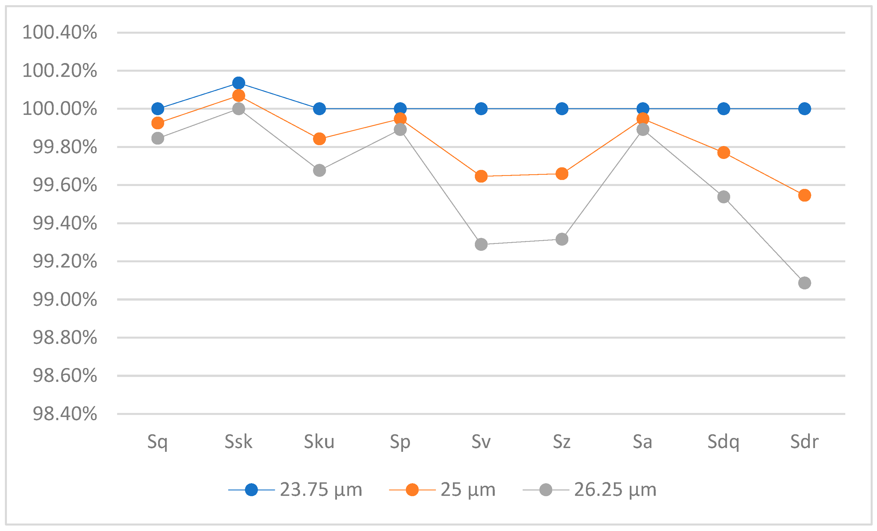
Results of applying a stylus size variation of ±5% to the 25 µm stylus for the groove standard with α = 130°.
Table 20.
Results of applying a stylus size variation of ±5% to the 25 µm stylus for the groove standard with α = 130°.
| Parameters | 23.75 µm | 25 µm | 26.25 µm |
|---|
| Sq [µm] | 3.2723 | 3.2699 | 3.2672 |
| Ssk | −4.0558 | −4.0531 | −4.0503 |
| Sku | 18.8292 | 18.7994 | 18.7684 |
| Sp [µm] | 0.8623 | 0.8618 | 0.8614 |
| Sv [µm] | 18.0135 | 17.9497 | 17.8853 |
| Sz [µm] | 18.8758 | 18.8115 | 18.7467 |
| Sa [µm] | 1.5791 | 1.5783 | 1.5774 |
| Sdq [rad] | 0.1311 | 0.1308 | 0.1305 |
| Sdr [%] | 0.8192 | 0.8155 | 0.8117 |
Table 21.
Results of applying a stylus size variation of ±5% to the 50 µm stylus for the groove standard with α = 130°.
Table 21.
Results of applying a stylus size variation of ±5% to the 50 µm stylus for the groove standard with α = 130°.
| Parameters | 47.5 µm | 50 µm | 52.5 µm |
|---|
| Sq [µm] | 3.2058 | 3.1965 | 3.1869 |
| Ssk | −3.9920 | −3.9841 | −3.9761 |
| Sku | 18.1443 | 18.0627 | 17.9804 |
| Sp [µm] | 0.8496 | 0.8478 | 0.8459 |
| Sv [µm] | 16.7986 | 16.6712 | 16.5441 |
| Sz [µm] | 17.6482 | 17.5190 | 17.3899 |
| Sa [µm] | 1.5558 | 1.5525 | 1.5490 |
| Sdq [rad] | 0.1253 | 0.1246 | 0.1240 |
| Sdr [%] | 0.7480 | 0.7405 | 0.7330 |
Table 22.
Results of applying a stylus size variation of ±5% to the 100 µm stylus for the groove standard with α = 130°.
Table 22.
Results of applying a stylus size variation of ±5% to the 100 µm stylus for the groove standard with α = 130°.
| Parameters | 95 µm | 100 µm | 105 µm |
|---|
| Sq [µm] | 2.9631 | 2.9300 | 2.8956 |
| Ssk | −3.8293 | −3.8120 | −3.7950 |
| Sku | 16.5542 | 16.3956 | 16.2410 |
| Sp [µm] | 0.7989 | 0.7916 | 0.7839 |
| Sv [µm] | 14.3941 | 14.1429 | 13.8921 |
| Sz [µm] | 15.1930 | 14.9345 | 14.6760 |
| Sa [µm] | 1.4628 | 1.4494 | 1.4353 |
| Sdq [rad] | 0.1126 | 0.1111 | 0.1097 |
| Sdr [%] | 0.6056 | 0.5906 | 0.5756 |
Table 23.
Results of applying a stylus size variation of ±5% to the 5 µm stylus for the peak standard with α = 130°.
Table 23.
Results of applying a stylus size variation of ±5% to the 5 µm stylus for the peak standard with α = 130°.
| Parameters | 4.75 µm | 5 µm | 5.25 µm |
|---|
| Sq [µm] | 3.2956 | 3.2956 | 3.2956 |
| Ssk | 4.0838 | 4.0838 | 4.0838 |
| Sku | 19.1491 | 19.1491 | 19.1491 |
| Sp [µm] | 19.1335 | 19.1334 | 19.1334 |
| Sv [µm] | 0.8665 | 0.8666 | 0.8666 |
| Sz [µm] | 20.0000 | 20.0000 | 20.0000 |
| Sa [µm] | 1.5868 | 1.5868 | 1.5868 |
| Sdq [rad] | 0.1361 | 0.1360 | 0.1360 |
| Sdr [%] | 0.8812 | 0.8808 | 0.8806 |
Table 24.
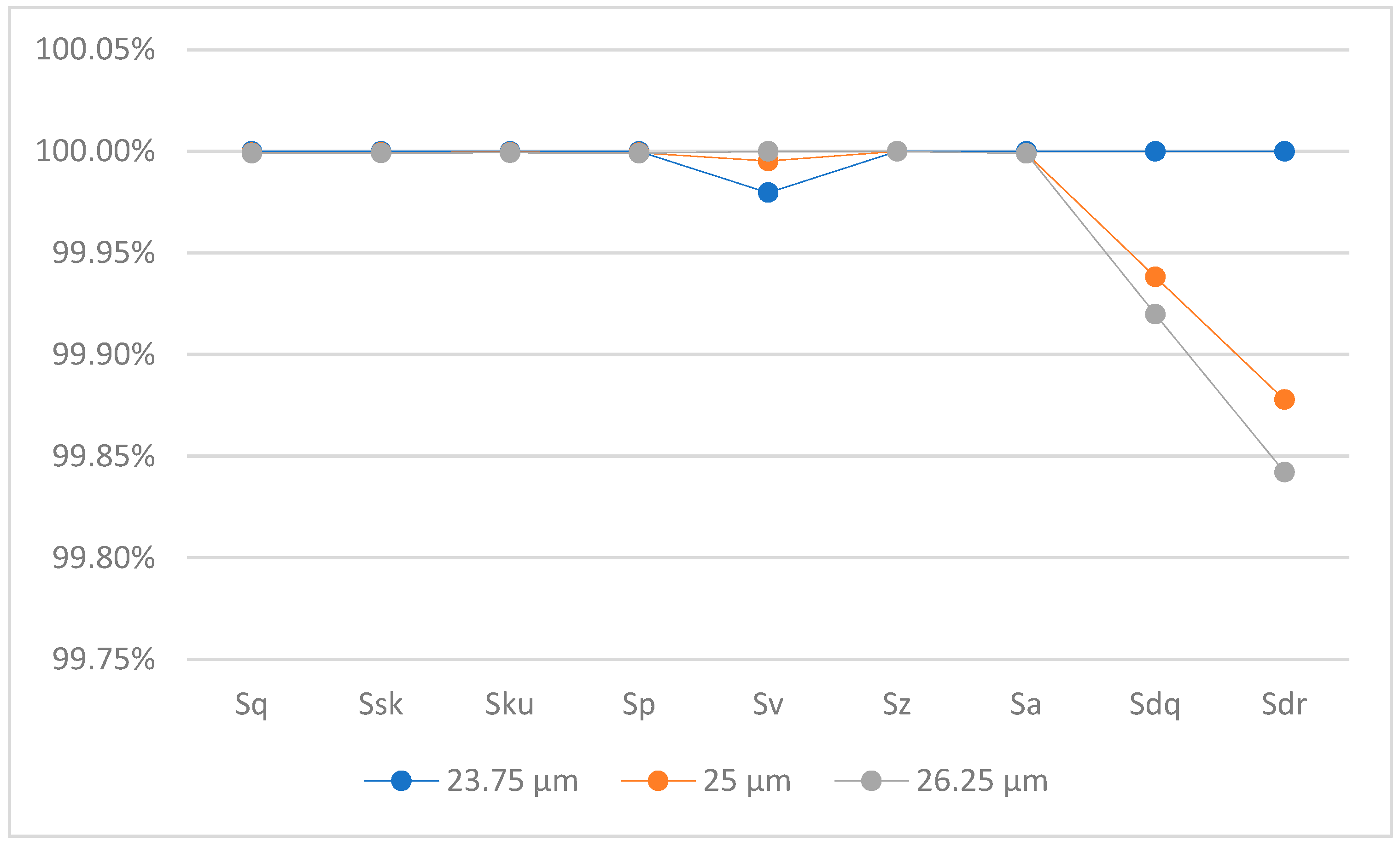
Results of applying a stylus size variation of ±5% to the 25 µm stylus for the peak standard with α = 130°.
Table 24.
Results of applying a stylus size variation of ±5% to the 25 µm stylus for the peak standard with α = 130°.
| Parameters | 23.75 µm | 25 µm | 26.25 µm |
|---|
| Sq [µm] | 3.2954 | 3.2954 | 3.2954 |
| Ssk | 4.0836 | 4.0836 | 4.0836 |
| Sku | 19.1484 | 19.1483 | 19.1483 |
| Sp [µm] | 19.1324 | 19.1323 | 19.1322 |
| Sv [µm] | 0.8676 | 0.8677 | 0.8678 |
| Sz [µm] | 20.0000 | 20.0000 | 20.0000 |
| Sa [µm] | 1.5867 | 1.5866 | 1.5866 |
| Sdq [rad] | 0.1350 | 0.1349 | 0.1349 |
| Sdr [%] | 0.8677 | 0.8666 | 0.8663 |
Table 25.
Results of applying a stylus size variation of ±5% to the 50 µm stylus for the peak standard with α = 130°.
Table 25.
Results of applying a stylus size variation of ±5% to the 50 µm stylus for the peak standard with α = 130°.
| Parameters | 47.5 µm | 50 µm | 52.5 µm |
|---|
| Sq [µm] | 3.2951 | 3.2951 | 3.2951 |
| Ssk | 4.0821 | 4.0818 | 4.0813 |
| Sku | 19.1405 | 19.1389 | 19.1365 |
| Sp [µm] | 19.1294 | 19.1289 | 19.1284 |
| Sv [µm] | 0.8706 | 0.8711 | 0.8716 |
| Sz [µm] | 20.0000 | 20.0000 | 20.0000 |
| Sa [µm] | 1.5875 | 1.5876 | 1.5880 |
| Sdq [rad] | 0.1337 | 0.1335 | 0.1333 |
| Sdr [%] | 0.8513 | 0.8491 | 0.8473 |
Table 26.
Results of applying a stylus size variation of ±5% to the 100 µm stylus for the peak standard with α = 130°.
Table 26.
Results of applying a stylus size variation of ±5% to the 100 µm stylus for the peak standard with α = 130°.
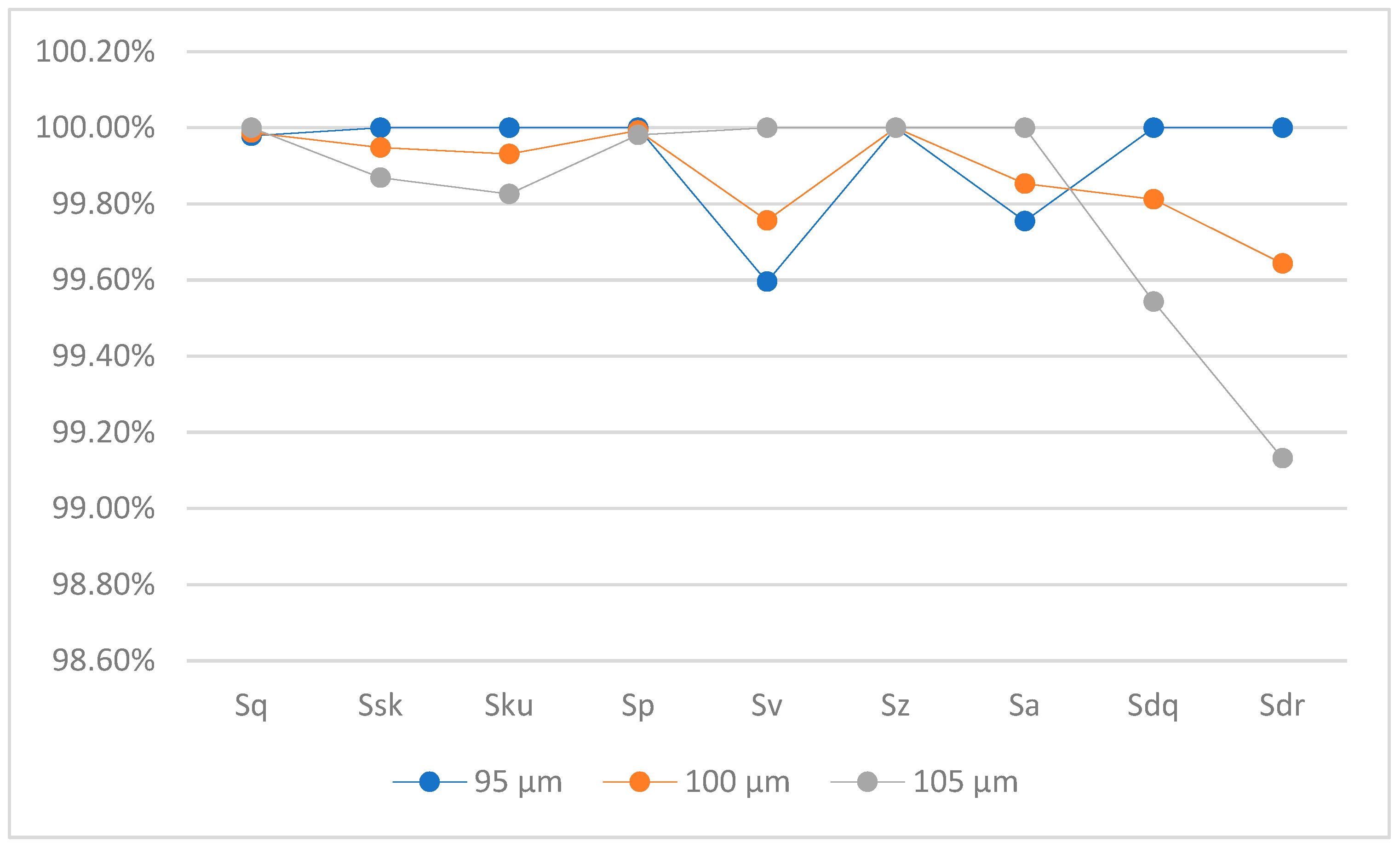
| Parameters | 95 µm | 100 µm | 105 µm |
|---|
| Sq [µm] | 3.2958 | 3.2960 | 3.2965 |
| Ssk | 4.0694 | 4.0673 | 4.0641 |
| Sku | 19.0663 | 19.0532 | 19.0331 |
| Sp [µm] | 19.1173 | 19.1158 | 19.1137 |
| Sv [µm] | 0.8827 | 0.8842 | 0.8863 |
| Sz [µm] | 20.0000 | 20.0000 | 20.0000 |
| Sa [µm] | 1.5972 | 1.5988 | 1.6011 |
| Sdq [rad] | 0.1309 | 0.1306 | 0.1303 |
| Sdr [%] | 0.8175 | 0.8146 | 0.8104 |


