Abstract
Traditional revolute clearance joints assume that the shape of the contact surface of the joint is regular and ignores the effects of wear, which reduces the prediction accuracy of dynamics models. To accurately describe the collision behavior of the motion pair, an Archard formula was applied to construct a wear clearance model. Based on the absolute node coordinate method, multi-body dynamics modeling, wear prediction, and chaotic identification analysis methods for a flexible multi-link mechanism with clearance considering wear effects were proposed. The research results indicate that wear exacerbates the irregularity of the clearance surface contours, leading to increased instability in the dynamic response and the reduced motion accuracy of the mechanism. Compared with clearance size, driving speed has a more significant impact on the chaotic behavior of the system. For high-speed conditions, maintaining the clearance size within approximately 0.1 mm is beneficial for system stability, although this requirement poses challenges for cost control in manufacturing. This study provides a theoretical foundation for wear prediction and stability optimization of high-precision multi-link mechanisms.
1. Introduction
In practical mechanical systems, clearance inevitably originates from design, manufacturing, wear, and assembly. The presence of clearance exacerbates the impact between components, resulting in severe vibration, friction, noise, wear, and elastic deformation, leading to chaotic characteristics [1,2,3]. The coupled degradation mechanism originating from progressive wear and component flexibility presents exceptional complexity, serving as a critical contributor to mechanical system failures [4,5,6,7]. Consequently, a systematic investigation of the wear–flexibility coupling mechanism becomes essential for the precise prediction of motion states and dynamic behaviors, particularly in understanding its influence on nonlinear dynamic responses.
Clearance seriously affects dynamic characteristics of mechanisms. While most scholars have regarded clearance in motion pairs as regular and constant, analyzing its effects on dynamic characteristics [8,9], the reality shows more complex behaviors. Guo et al. [10] demonstrated that rotational speed increases peak responses and vibration frequencies in rudder loops, while larger clearances reduce vibration frequencies but increase response errors. An increase in clearance value increases response errors but reduces vibration frequency. Bai et al. [11] built clearance models for both rotating and translational pairs, and discussed the coupling effect of these two clearances on the dynamics of crank slider mechanisms. Zhang et al. [12] studied the dynamics of a vehicle shear door mechanism with various clearances. Chouaibi et al. [13] analyzed the impact of clearance on the accuracy of RAF robots and DELTA robots, and found that RAF robots have a greater sensitivity to clearance. Korayem et al. [14] investigated the maximum load capacity of robotic manipulators by considering the flexible joint under various base positions and predefined trajectories. Song et al. [15] investigated the comprehensive coupling effects of component flexibility, various clearances between motion pairs, and lubrication on dynamical behaviors in mechanisms. Wang et al. [16] revealed the influence of clearance size, crankshaft speed, and lubricant viscosity coefficients on the dynamic behavior of the mechanism under lubrication and dry friction conditions. Jiang et al. [17] investigated bifurcation maps of vehicle shimmy systems considering clearance joints. Wu et al. [18] evaluated the chaotic system behavior of crank slider mechanisms corresponding to different clearance sizes and crank speeds through bifurcation analysis. The issue of system reliability degradation caused by clearances has also attracted significant attention from researchers, Yang et al. [19] applied an improved PSO algorithm to optimize the parameters of the manipulator, reducing the effect of clearance on the accuracy of the mechanism. Cheng et al. [20] proposed a time-varying motion reliability methodology that comprehensively considers clearance and random variables, and applied it to typical four bar mechanisms and single crank double rocker mechanisms to verify its effectiveness. Jiang et al. [21] proposed a dynamic analysis approach for robot mechanisms considering interval parameters and studied the effects of clearance and uncertainties on their dynamics. Jia et al. [22] studied the reliability analysis of parallel mechanisms containing clearances and uncertainties. These studies have advanced the understanding of nonlinear dynamic characteristics in mechanical systems with clearances, yet they have largely overlooked the essential fact that clearances are inherently dynamic in nature.
Mechanical equipment needs to run many motion cycles during use, and joints inevitably wear out, resulting in uneven clearance between motion pairs, which has attracted the attention of scholars [23,24,25]. Mukras et al. [26] used the Archard model to iteratively predict the wear of joints, and compared the theoretical wear prediction results with the wear results on the crank slider experimental platform to verify the accuracy of the prediction. Lopez-Lombardero et al. [27] proposed a wear simulation approach for rotating joints in a crank slider mechanism considering the flexibility of the connecting rod. Wang et al. [28] took the classic four bar mechanism as an example to discuss the irregular wear law of pairs. Ordiz et al. [29] put forward a simplified method to analyze the influence of clearance wear on the service life of machines. Li et al. [30] applied a contact surface discretization approach to reconstruct the surface of a motion pair after wear. Jiang et al. [31] proposed a reliability methodology for motion mechanisms considering multiple wear joints. Zhao et al. [32] developed a model for flexible components using the Absolute Nodal Coordinate Formulation (ANCF) and investigated wear phenomena in the revolute joints of flexible multibody systems. Gao et al. [33] proposed an immune algorithm optimization approach to reduce the influence of wear on dynamics of crank slider mechanisms. Zhuang et al. [34] conducted motion reliability analysis on a planar mechanism with a wear pair, and verified wear prediction approach through experimental testing. Zhuang et al. [35] conducted a reliability analysis for dual axis drive mechanisms with wear clearance. Liu et al. [36] took linkage motion mechanisms on industrial assembly lines as an example, and studied the wear process and failure model of a multi-body mechanism considering wear and plastic deformation. Hou et al. [37] built a dynamic model of a 3RSR parallel mechanism with spherical wear clearance, and analyzed wear effect caused by long-term operation. As a typical source of nonlinearity, the impact effects induced by clearances render systems with clearances distinctly nonlinear. Particularly, the nonlinear characteristics arising from time-varying clearances have become a crucial factor that cannot be overlooked in this research field
Previous studies have predominantly been based on two critical assumptions regarding the constancy and regularity of clearance values along with the ideal rigid-body behavior of system components. However, these assumptions fail to adequately account for the impact of irregular clearance variations caused by wear on motion accuracy, as well as vibration issues resulting from the elastic deformation of components, leading to significant deviations in dynamic analysis. In particular, existing approaches often overlook the coupled effects of wear evolution and component flexibility on system chaos characteristics. Addressing these limitations, this study proposes an innovative methodology that enables a synergistic analysis of wear prediction and chaos identification in flexible mechanisms. This approach not only provides more accurate predictions of mechanical system operational states but also establishes a novel theoretical framework for investigating dynamic characteristics of complex mechanical systems.
The specific arrangement of this article is as follows: Section 2 establishes the irregular wear model; Section 3 builds a flexible beam model; Section 4 establishes a dynamic model of a flexible mechanism considering irregular wear clearance; Section 5 analyzes the effects of wear clearance on the dynamic and chaos characteristics of the mechanism and studies the influence of initial clearance values and driving speeds on the dynamic and chaos characteristics of the mechanism; and Section 6 provides the conclusion.
2. Establishment of Irregular Wear Model
2.1. Establishment of Ideal Revolute Clearance Model
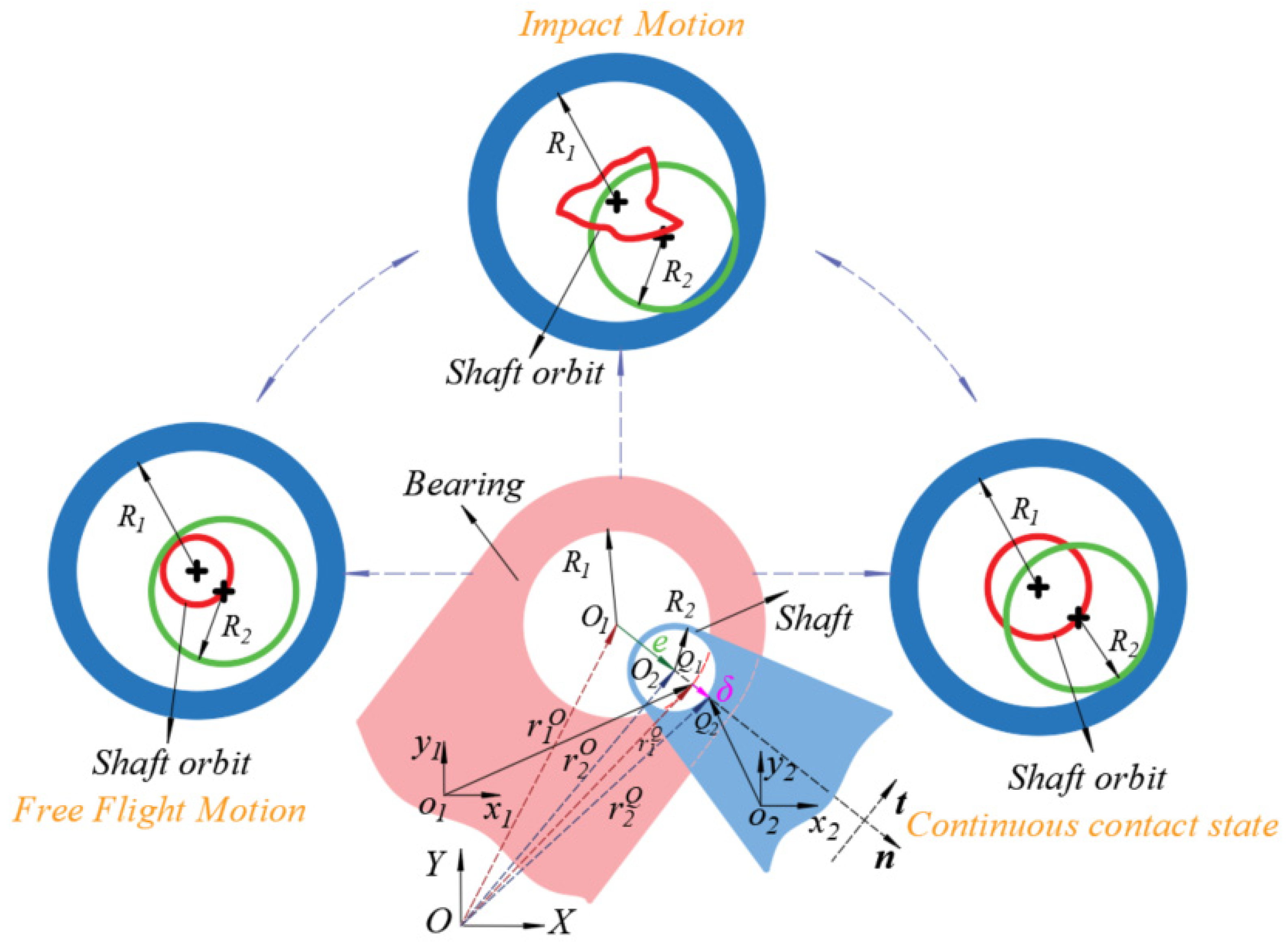
As displayed in Figure 1, the eccentricity vector between the shaft and bearing is
where and are the position vectors of the center of the bearing and shaft, respectively, and the length of eccentricity vector is [38]
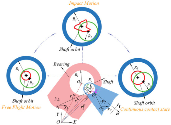
Figure 1.
Motion state of clearance motion pair.
The amount of deformation generated by collisions is as follows [39]:
where and are position vectors of contact points and , and c is the clearance joint value. According to deformation, the contact state of the shaft is determined. The shaft has three motion states in the bearing, as shown in Figure 1.
According to the actual contact state of the pair elements, the clearance contact surface could be represented by the contact force of the shaft in the bearing based on L–N contact theory [40]
where K is the stiffness coefficient, and are the penetration depth and relative normal contact velocity, and D is the hysteresis damping factor.
The stiffness coefficient can be expressed as [5,11]
where the Young’s modulus E* is related to the elastic moduli E1 and E2 of the bearing and shaft, as well as the Poisson’s ratios υ1 and υ2, which can be expressed as
Hysteresis damping factor D is determined by the material’s recovery coefficient ce and ; it can be written as
Due to the frequent changes in tangential velocity at the hinge, to overcome the unstable numerical solution of the Coulomb model, a dynamic correction coefficient was introduced to obtain the Ambrosio friction force model, which can be written as [18]
where is the coefficient of friction, is the dynamic correction coefficient, and its expression is
where and are given a speed limit value.
2.2. Establishment of the Wear Clearance Model
When collision and wear occur on the surface of the motion pair elements, it is easy to cause sliding deformation and mutual compression in the motion pair. The Archard wear model establishes a theoretical framework where wear volume is proportional to normal load and sliding distance while being inversely proportional to material hardness, with a wear coefficient accounting for factors such as interface temperature and material properties. The loss can be calculated as
where V, s, and k represent wear volume, slip distance, and wear coefficient, respectively.
For the convenience of measuring relevant wear parameters, divide both sides of Equation (10) by the contact area between the shaft and bearing, use wear depth instead of wear volume, and use normal load instead of normal collision force. Equation (10) could be expressed as [41]
During the movement of the mechanism, the contact force, contact position, and sliding distance between shaft and bearing are constantly varying. Introducing wear rate dh can facilitate the calculation of accumulated wear, and Equation (11) can be written as
where dh and ds represent wear depth and slip distance per unit time, respectively.
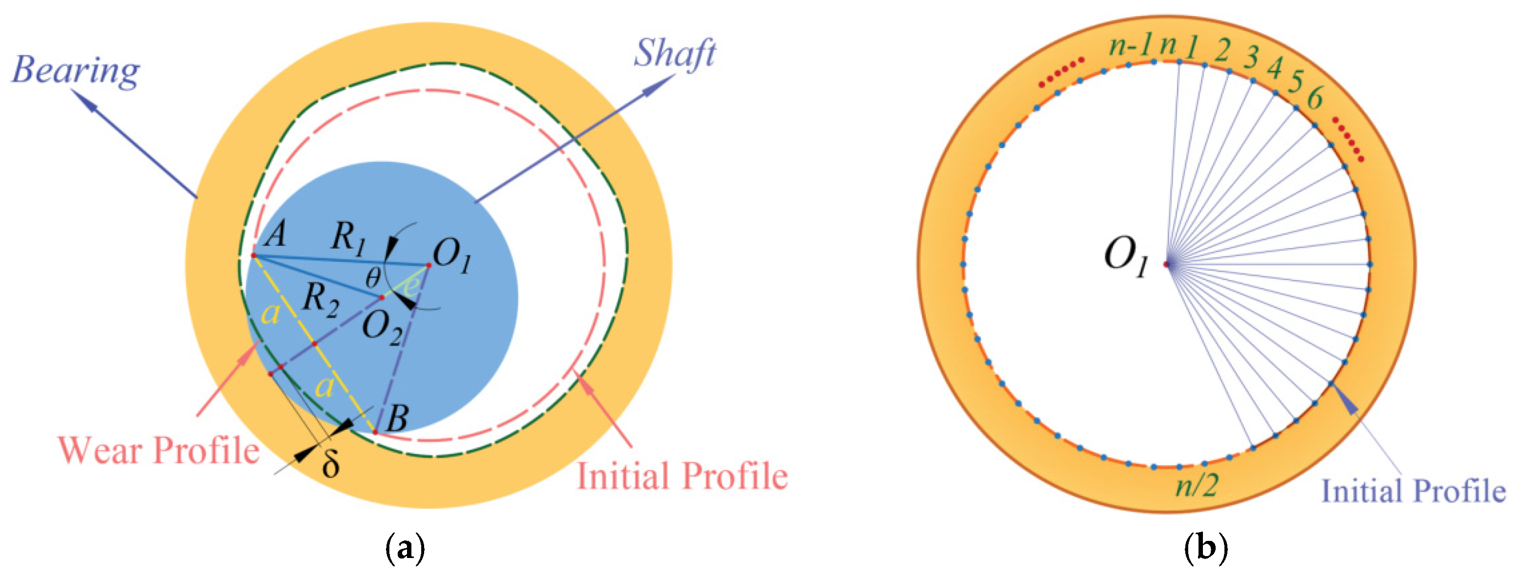
According to Figure 2a, the contact area between shaft and bearing are
where L is the axial contact length of hinge and a is the contact half width, which can be expressed as

Figure 2.
Wear analysis model. (a) Model of wear joint; (b) Surface of bearings after discretization treatment.
To achieve numerical calculations, based upon the finite element method, the surface area of the pair was discretized, as shown in Figure 2b. Based upon wear depth, the geometric surfaces of the worn axle and bearing could be obtained, and the total amount of wear depth is
where n is discrete area code, and hn is the wear depth within the discrete area code n.
The curvature radius at the discrete region n of the bearing is defined as , and the curvature radius at the discrete region n of the shaft is defined as . Clearance size at discrete region n could be written as
When the shaft moves in the bearing, the relative embedding depth of any potential collision point is a function of the clearance size. Therefore, the relative embedding depth at the discrete region n after wear is marked as . The normal collision force of the contact point after wear is expressed as
where the stiffness coefficient and hysteresis damping factor after wear are
When the shaft wears due to movement in the bearing, friction force at clearance is as follows
3. Establishment of Flexible Beam Element Model
The Absolute Nodal Coordinate Formulation (ANCF) possesses a constant mass matrix and can accurately describe large rotations, large deformations, and cross-sectional deformations of flexible bodies, making it extensively applicable in the study of flexible multibody systems. Based on ANCF, a model of flexible components was established, and a schematic diagram of the flexible component structure is shown in Figure 3. The absolute position vector r of any point on the element could be derived by the absolute node coordinates ef and the shape function S of the nodes at both ends of the element
where r1 and r2 are coordinate components of any point along the X and Y axes, respectively. S can be written as
where l is the unit length, and si(1, 2, 3, 4) can be expressed as [42]
where , x is the local coordinate of any point before deformation, .
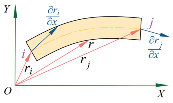
Figure 3.
Flexible member model.
Generalized coordinates of flexible elements can be expressed as
where , , , , , , , .
The mass matrix of elastic beam elements can be expressed as
where ρ and A represent density and the cross-sectional area of the flexible element.
The stiffness matrix of the beam elements can be expressed as
where Kl and Kt represent the tensile and compressive stiffness and bending stiffness of the unit, respectively, , I is the moment of inertia of the section, and is strain.
The strain of the flexible element is as follows
The elastic force of a flexible beam element is the vector sum of the axial elastic force and bending elastic force
The dynamic equation of the flexible element is as follows
where is the generalized force of the flexible beam element.
4. Dynamic Model for Mechanism with Irregular Wear Clearance
A schematic diagram of the six bars mechanism is displayed in Figure 4. It has five active components, namely L1, L2, L3, L4, and S5. L1 is crank, L2 is triangle plate, L3 and L4 are rods, and S5 is slider. Due to the longer length of rods 3 and 4, they are more prone to elastic deformation compared with other components. Therefore, flexible treatment is applied to rods 3 and 4. Rotating pair A is an important motion pair connecting the entire driving component of the mechanism. Therefore, considering clearance A can better reflect the impact of the clearance on the mechanism.
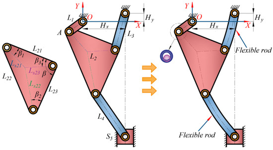
Figure 4.
Structural diagram of six bars mechanism.
4.1. Establishment of Dynamic Model for Mechanism with Irregular Wear Clearance
Since components 1, 2, and 5 are considered rigid components, and components 3 and 4 are considered flexible components, the generalized coordinates of each component are as follows
Therefore, the generalized coordinates of the entire system are
where is the generalized coordinate of the system’s rigid components, , and is the generalized coordinate of the flexible components, .
Constraint equation of mechanism can be written as
where ω is the angular velocity of the crankshaft.
The velocity constraint equation could be obtained by taking the first derivative of Equation (33) with respect to time
where is the Jacobian matrix, .
The Jacobian matrix can be represented as
where is the derivative of the constraint equation with respect to the generalized coordinates of the rigid components, , and is the derivative of the constraint equation with respect to the generalized coordinates of the flexible components, .
The acceleration constraint equation can be obtained by taking the first derivative of Equation (34) with respect to time
where is the generalized acceleration vector of the system, , .
The dynamic model of the system could be represented as [43]
where and are the mass matrix and total external force of the rigid components, λ is the Lagrange multiplier, , , and are the mass matrix, total external force, and elastic force of the flexible components, respectively.
To solve problems of default and calculation divergence when solving equations, Baumgarte proposes a default stabilization algorithm that incorporates displacement and velocity constraints into the acceleration constraint equation to improve solution stability [22,32]. The objective of the Baumgarte method is to replace the acceleration constraint equations (Equation (36)) with
where α and β are the Baumgarte feedback parameters.
4.2. Establishment of Chaos Characteristics Identification Model
The maximum Lyapunov exponent (MLE) is one of the key indicators for identifying chaotic systems. By calculating the maximum Lyapunov exponent, we can quantitatively assess the degree of chaos in a system and distinguish deterministic chaos from external noise or topological complexity. The Lyapunov exponent quantitatively describes the rate at which two initially close trajectories diverge over time. If the maximum Lyapunov exponent of a system is positive, the system is defined as chaotic. In this study, we use the Wolf algorithm [44] to compute the maximum Lyapunov exponent. By calculating the dynamic model considering irregular wear clearance, motion states at clearance are obtained, which are components of the eccentricity vector between the shaft and bearing in the X and Y directions. Based on the eccentricity vector between the shaft and bearing in the X and Y directions, we can calculate the average period, time delay, and embedding dimension corresponding to these data, and use the method of reconstructing phase space. This series of data can be represented as
where m is the embedding dimension and τ is the time delay, which can be estimated by the C-C method.
Take the starting point as and take any point near the starting point as , and the length between the two points is . As time goes by, the distance between these two points also changes again. When the value between the two points is greater than the specified value ε(ε > 0) at time t1, and the length is , then is retained and another point is found near , making and minimizing the angle between the two points. Repeat the above process until the endpoint N of the time series is reached. MLE can be obtained by the following formula [40]
where M is the total number of iterations, tm is the time corresponding to the Mth iteration, and t0 is initial time.
5. Dynamic Analysis of Mechanical System
In actual working conditions, the motion pairs with irregular contours formed by wear affect the force and motion transmission between moving components, ultimately leading to a decrease in the motion accuracy and dynamics of the mechanism. The main purpose of this section is to explore changes in dynamic performance caused by irregular wear clearances and the evolution law of the contour surface of clearance pairs. The research content includes comparing and analyzing the dynamic characteristics of mechanisms containing irregular wear clearances and dry friction clearances and conducting chaos identification. The influence of clearance value and motion speed on dynamic response and the chaotic characteristics of mechanisms with irregular wear clearances were studied. To reduce calculation time, the mechanism first ran 100 cycles to obtain the wear depth of the clearance motion pair, and then expanded the data of 100 cycles to 10,000 times for wear analysis, to more clearly see the impact of wear on the surface of the motion pair and its dynamic response.
5.1. Simulation Parameters
The simulation parameters of the flexible multi-link mechanism with irregular wear joints are displayed in Table 1. Simulations were carried out using MATLAB (MATLAB R2018b), with the fourth-order Runge–Kutta method employed to solve the differential equations. The integral tolerance was set to 1 × 10⁻⁶, and the integral step size was related to the motion period, with each period divided into 10,000 steps, i.e., (2π/ω)/10,000.

Table 1.
Simulation parameters of a flexible multi-link mechanism with irregular wear clearance joint.
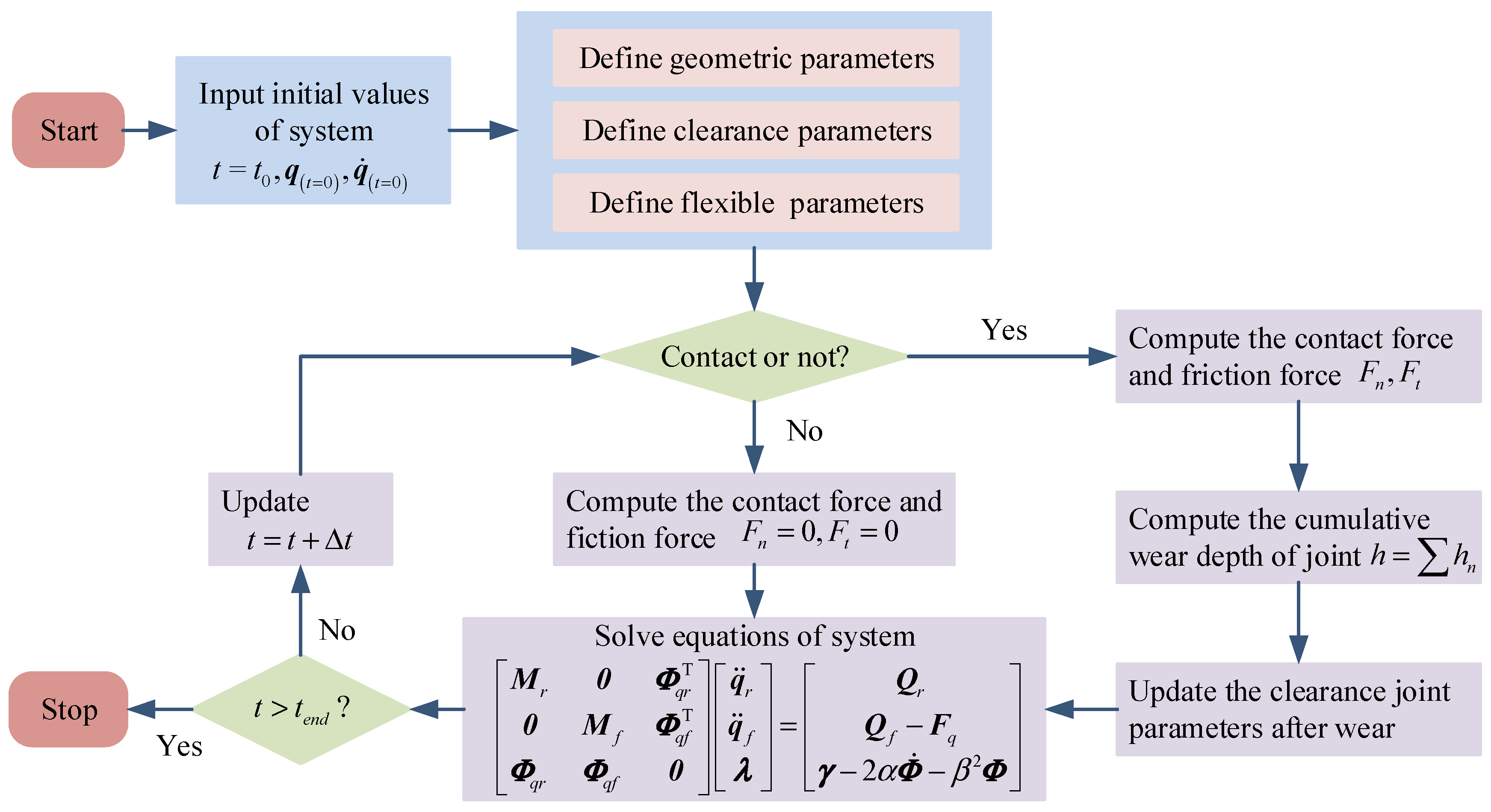
5.2. Solution Flowchart
A flowchart for solving the dynamic equation is shown in Figure 5.
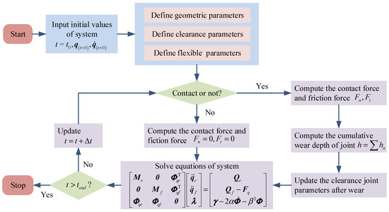
Figure 5.
Flowchart for solving dynamic equation.
The steps of the flowchart for solving dynamic equations in the mechanism can be summarized as follows:
- Start simulation with given initial values of system for positions and velocities .
- Define the geometric parameters, clearance parameters, and flexible parameters of the system to ensure the model accurately reflects the physical characteristics of the mechanism.
- Determine whether the contact exists between the joint element. If there is contact, calculate the contact force Fn and friction force Ft, further compute the wear depth, and update the parameters of the clearance joint. If no contact exists, set the contact force Fn and friction force Ft to zero.
- Solve the dynamic response of the system based on Equation (38).
- Determine whether the current time exceeds the end time. If yes, terminate the computational process, if no, update the current time to and obtain the new generalized positions and velocities of the system in the next step.
5.3. Comparative Analysis of Mechanism Dynamics Before and After Wear
This section analyzes the dynamic characteristic curves of the mechanism before and after wear, assuming the driving speed of the crankshaft is 150 rpm and the clearance value is 0.2 mm. In this study, ANCF was employed to model 2D beam elements, with rods 3 and 4 discretized into varying element counts as detailed in Table 2. Maximum strain calculations were performed on rods 3 and 4 to verify mesh convergence, while maintaining an optimal balance between computational accuracy and efficiency. Based on these considerations, each flexible component was discretized into 16 elements. Beam element model diagram divided into 16 units are shown in Figure 6.
Table 2.
Mesh convergence test.
Figure 6.
Beam element model divided into 16 units.
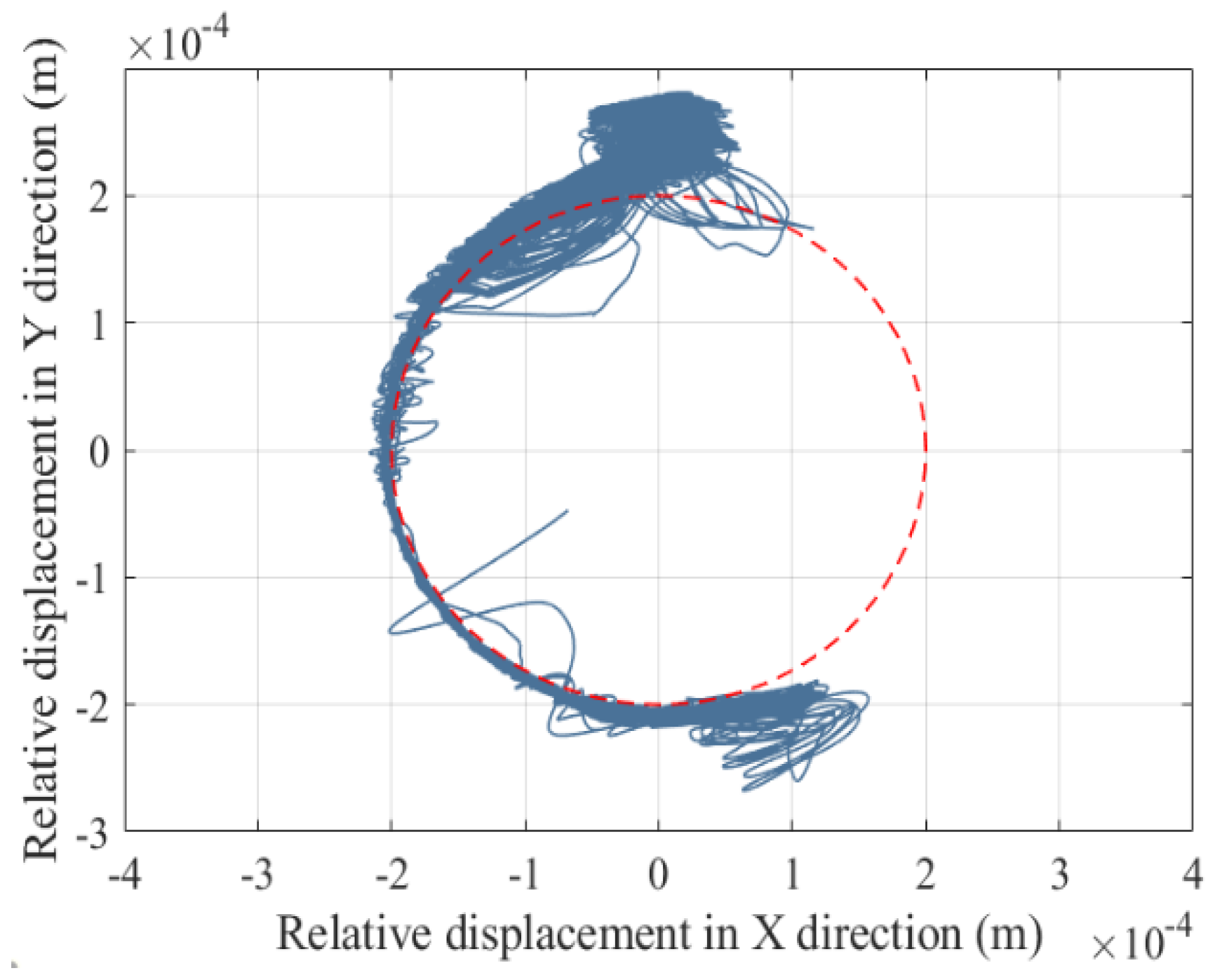
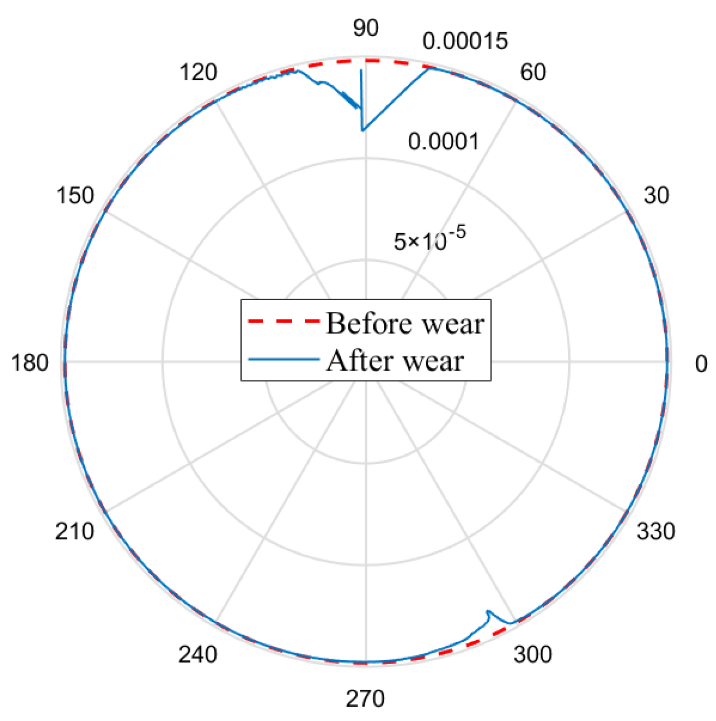
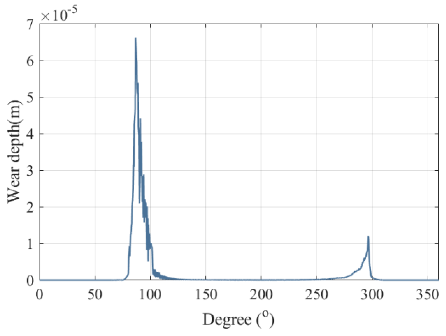
When the mechanism operates for 100 cycles, the center trajectory map at the clearance and embedding depth map are obtained, as shown in Figure 7 and Figure 8. By expanding the wear depth obtained from these 100 cycles by 10,000 times, we reconstructed the bearing surface based on this, and obtained an approximate wear depth of the mechanism running for 1 million cycles, as shown in Figure 8 and Figure 9, respectively. According to Figure 8 and Figure 10, the frequent collision area of the shaft in the bearing is the main wear area, and it was found that the wear of the bearing was not uniform. The wear area was mainly concentrated in [75°, 132°] and [252°, 310°]. The maximum wear depths in these two areas were 6.617 × 10⁻⁵ m and 1.204 × 10⁻⁵ m, respectively. This non-uniform wear pattern is associated with localized contact stress concentrations and dynamic load distribution, reflecting the nonlinear evolution characteristics of the clearance surface profile during long-term operation.

Figure 7.
Center trajectory before wear.
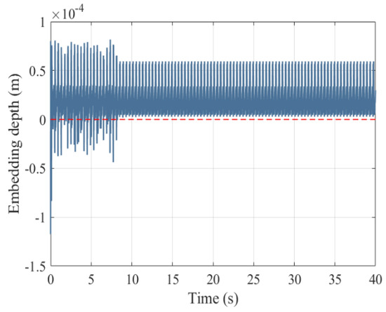
Figure 8.
Embedded depth before wear.
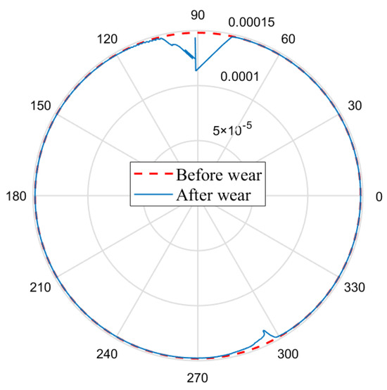
Figure 9.
Reconstruction of shaft surface.
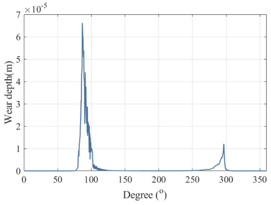
Figure 10.
Wear depth.
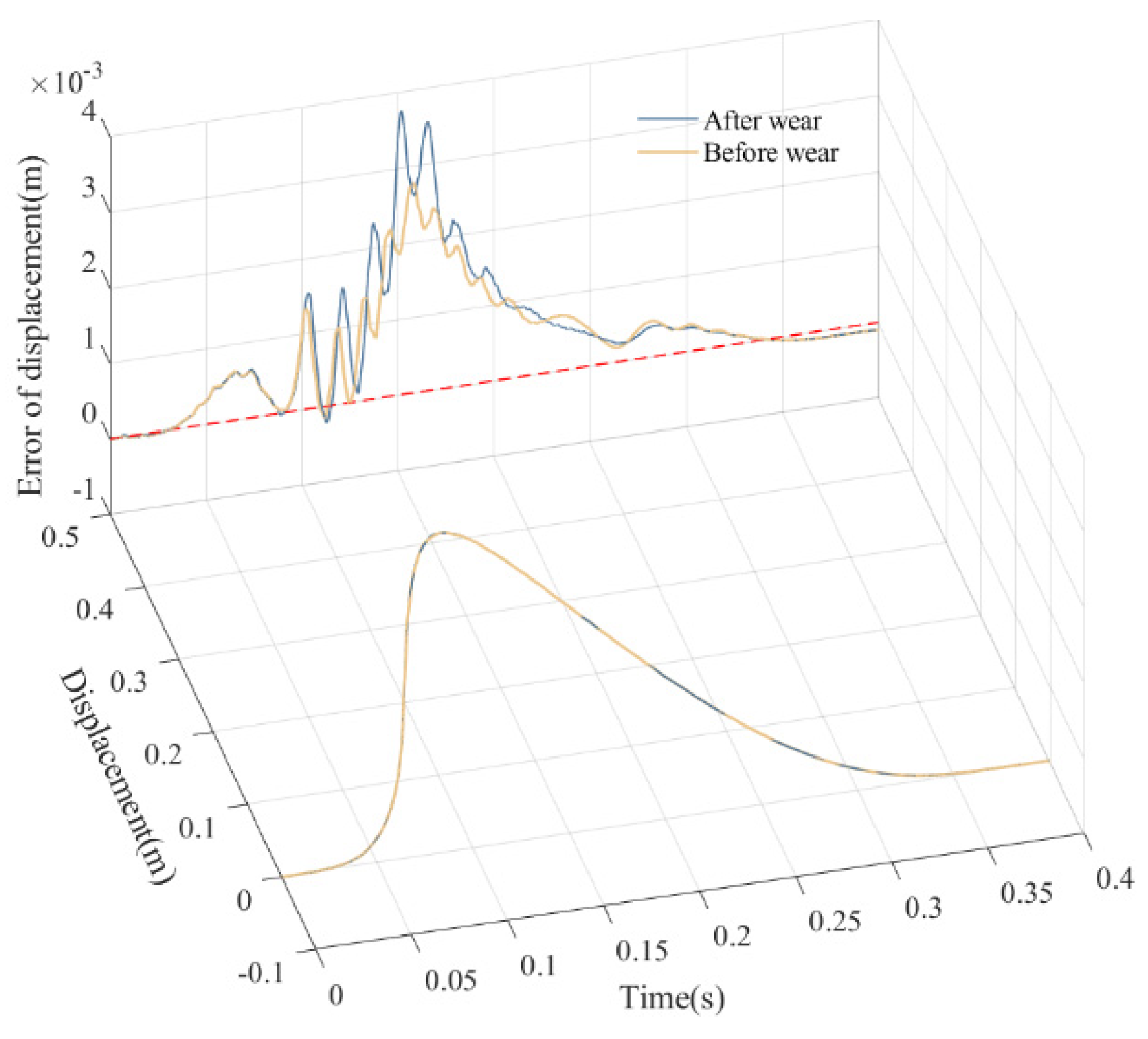
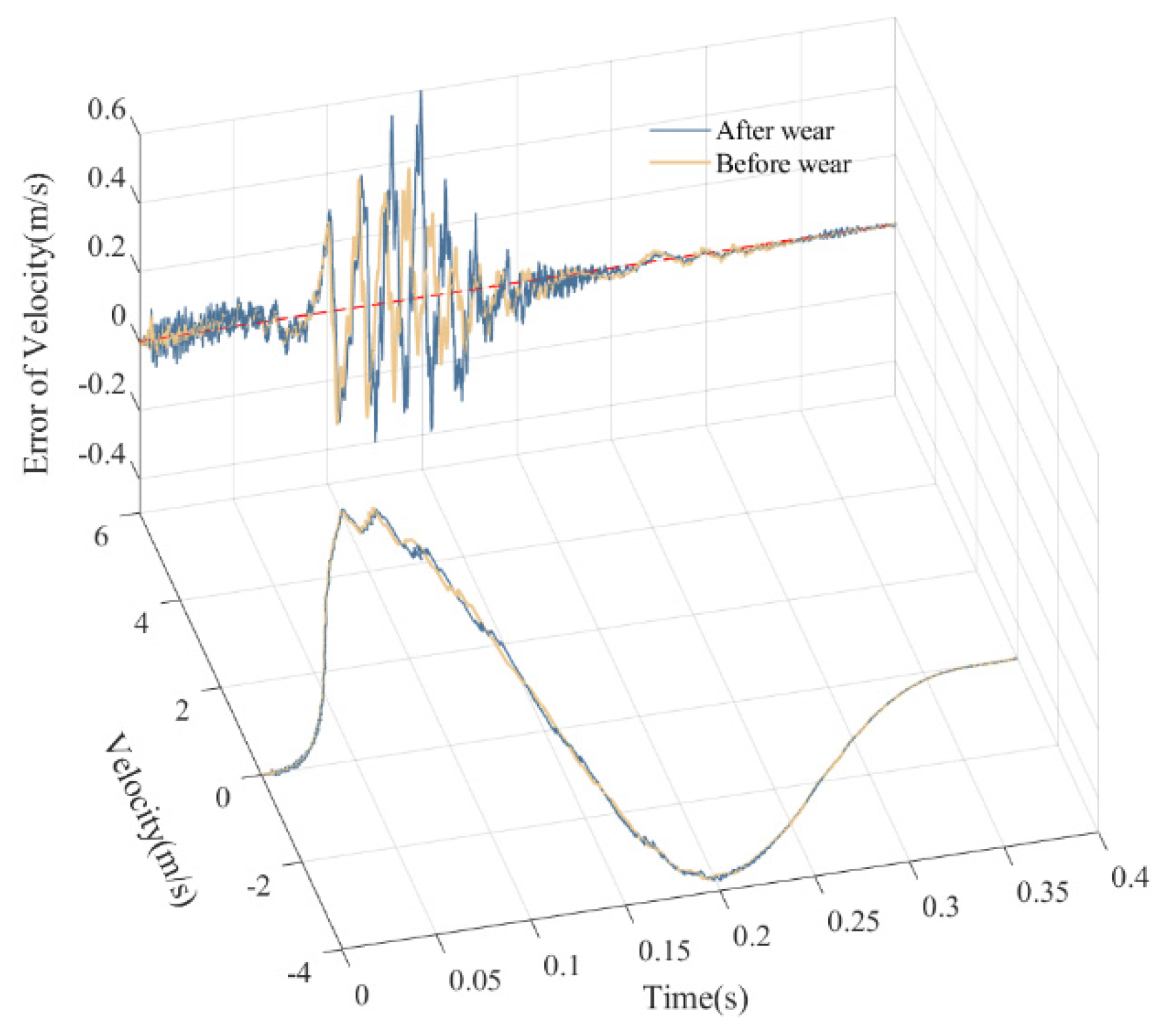
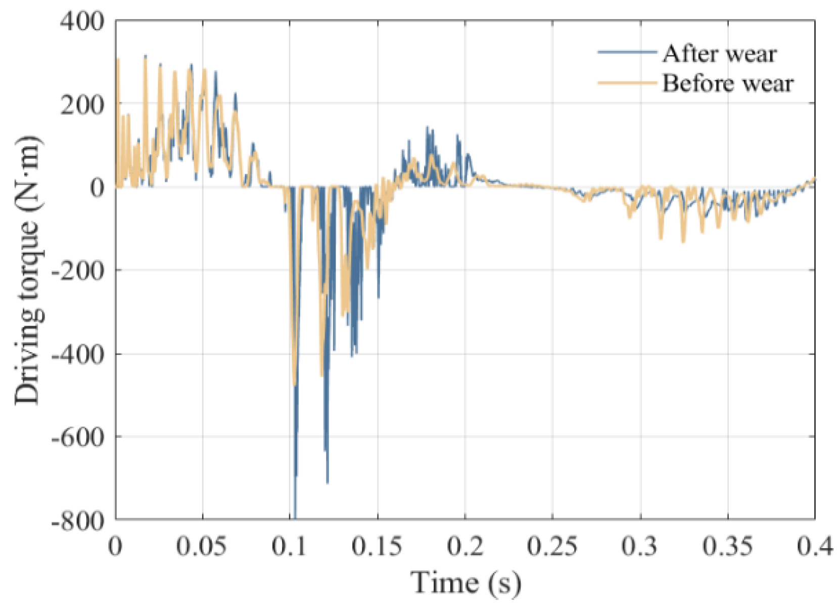
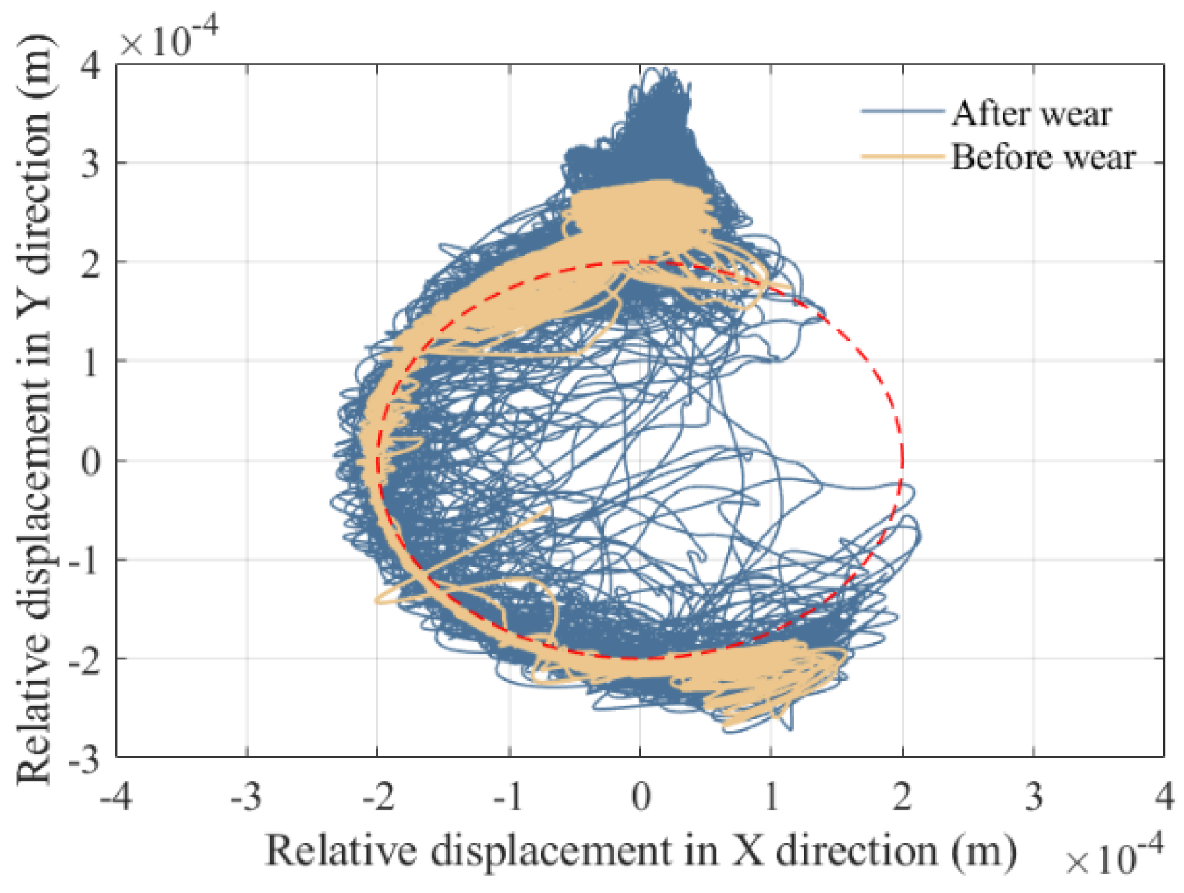
The peak dynamic response before and after wear is shown in Table 3. According to Figure 11 and Figure 12, the motion characteristic curves are displacement, displacement error, velocity, and velocity error, respectively. According to the displacement error curve, there is a certain increase in displacement error after wear, with an approximate rise of 1 mm. From the velocity error curve, it can be inferred that wear exhibits significant sensitivity to high-frequency dynamic characteristics, which is likely attributed to the transient collision forces at the clearance exciting the system’s high-frequency modes. As a result of wear, the velocity error has increased by 57.3%. The collision force, embedding depth, and driving torque curves are displayed in Figure 13 and Figure 14. The collision force increased by 14 kN, while the embedding depth and driving torque rose by 0.06 mm and 321.2 N·m, respectively. The increase in embedding depth after wear significantly amplifies the peak collision force, thereby driving a synchronous rise in the driving torque. This alteration in the energy transfer chain exacerbates the elastic deformation of the flexible rod, resulting in a strong synchronization between the strain curve and the collision force. Additionally, the rise in peak strain may accelerate the degradation of the material’s fatigue life. As shown in Figure 15, the strain curves of flexible rods 3 and 4 before and after wear are consistent with the collision force curve. Due to the intensified system impact caused by wear, rod 3 is more prone to deformation, with its strain increasing by 53.7 µm, while rod 4 shows a slight strain increase of 9.3 µm. According to Figure 16, it is noteworthy that wear also accentuates the nonlinear behavior of the system, as the chaotic nature of the clearance center trajectory reflects a change in the structure of the phase space attractor. Moreover, due to the increased vibration frequency and peak value of collision force after wear, the embedding depth of the shaft and bearing significantly increases.
Table 3.
Maximum value of dynamic before and after wear.
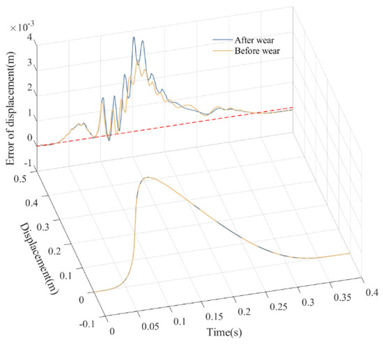
Figure 11.
Displacement and displacement error.
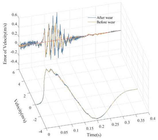
Figure 12.
Speed and speed error.
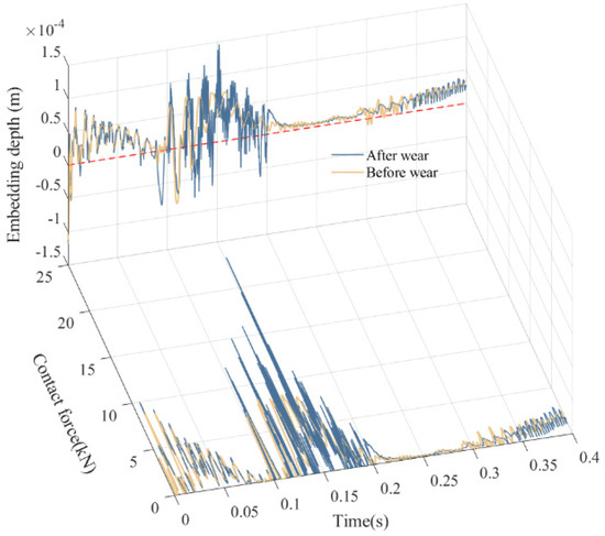
Figure 13.
Contact force and embedding depth.
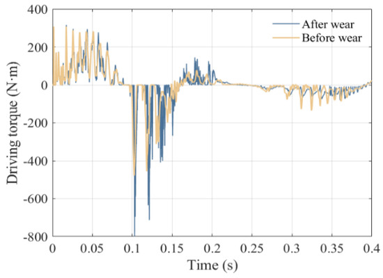
Figure 14.
Driving torque.
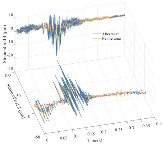
Figure 15.
Strain of flexible members.
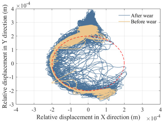
Figure 16.
Central trajectory.
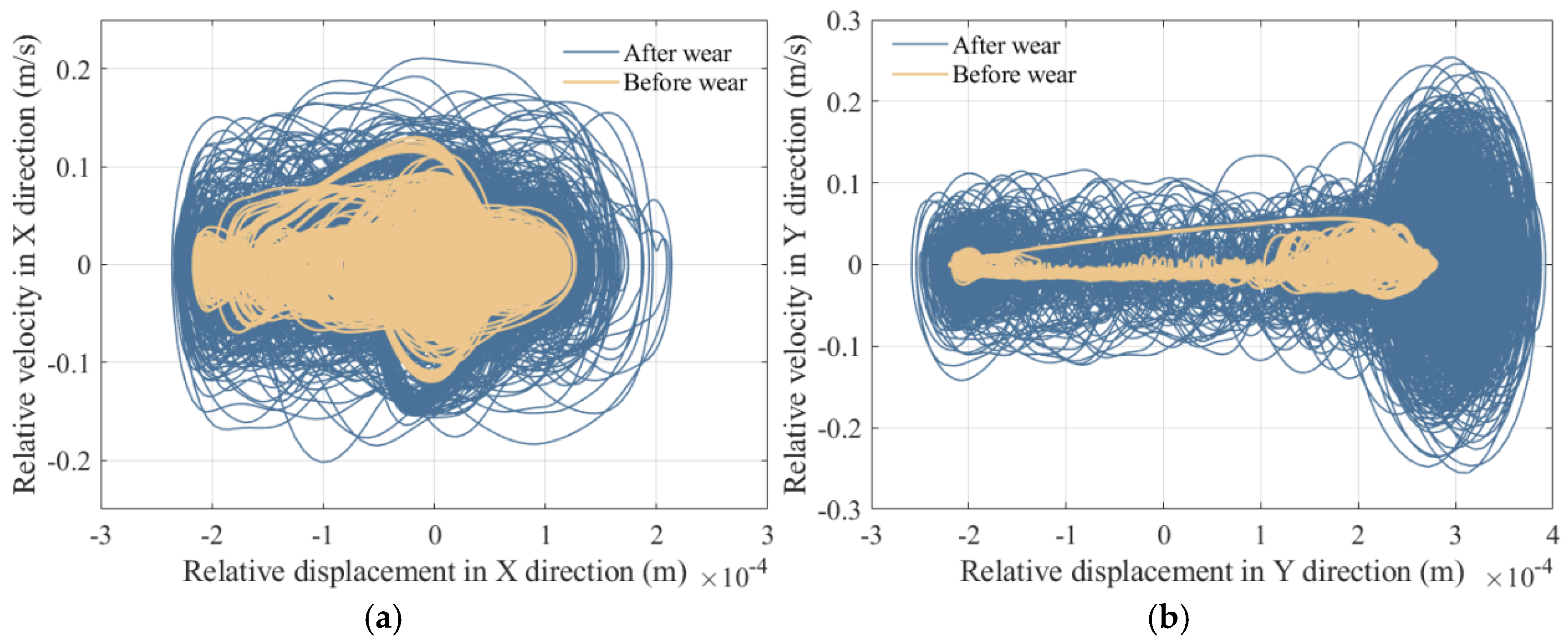
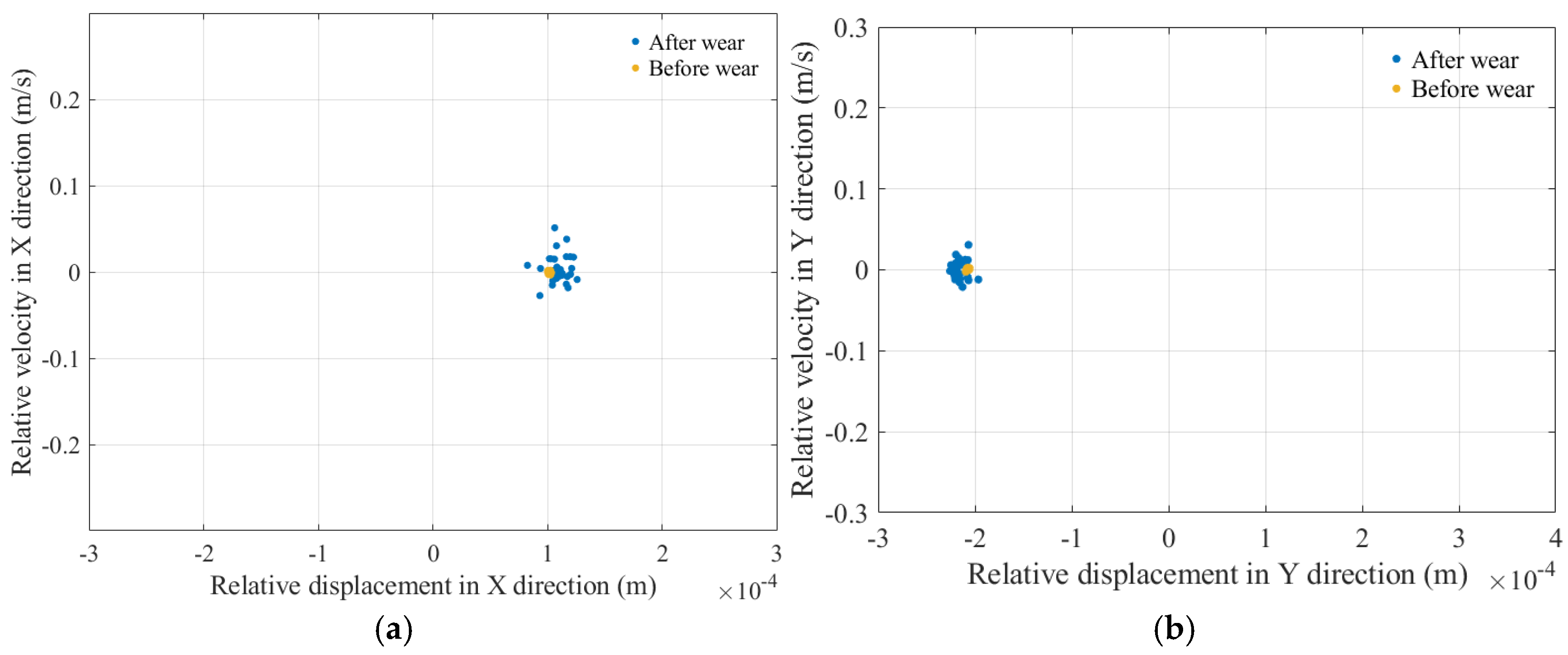
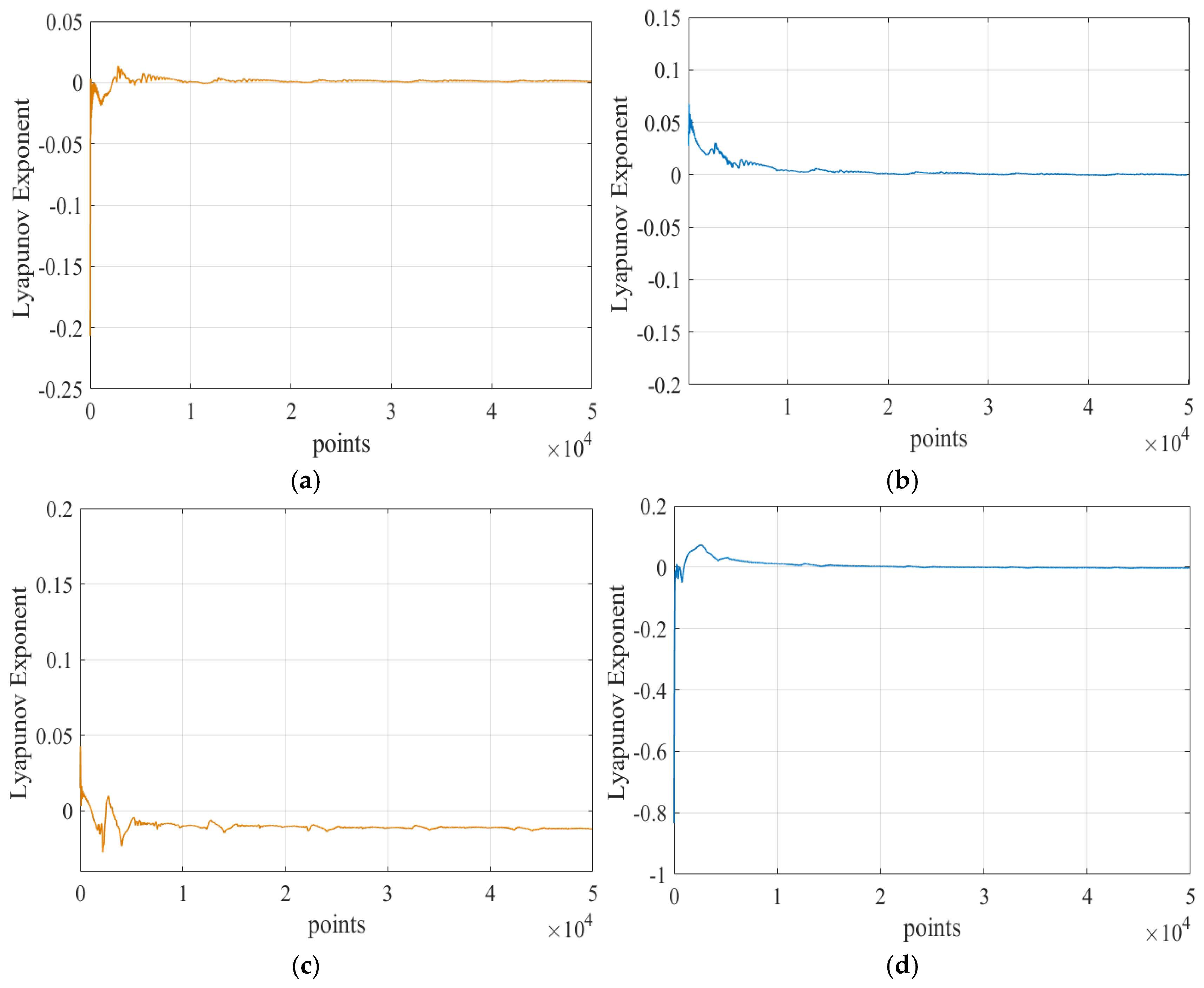
Before and after wear, the nonlinear characteristics of the motion state of the shaft in the bearing were studied based on motion state at the clearance, mainly including a phase diagram, Poincaré mapping diagram, and maximum Lyapunov exponent (MLE) diagram. The phase diagram and Poincaré mapping diagram displayed in Figure 17, Figure 18 and Figure 19 show that, compared with the before-wear condition, the after-wear trajectory becomes significantly scattered and complex, with the dispersion of Poincaré mapping points notably increasing, particularly in the X direction. Overall, the phase trajectory occupies a larger distribution space in the X direction compared with the Y direction, and the Poincaré mapping points also exhibit a broader distribution range, indicating higher sensitivity of the X direction to the wear behavior of the kinematic pair. This is primarily attributed to the uneven clearance distribution caused by wear, where localized clearance increases lead to variations in nonlinear contact stiffness and intensified impact vibrations. The expanded distribution area and enhanced irregularity of the after-wear phase trajectory are directly correlated, further reflecting a decline in system stability and a significant rise in chaotic behavior. To quantitatively assess the nonlinearity of the system, the MLE of the center trajectory time series was calculated, Parameter values for nonlinear characteristic evaluation are shown in Table 4. The results show that the MLE values in the X-direction before and after wear are 0.001 and 0.0042, respectively, while those in the Y-direction are −0.01 and 0.0047. The significant increase in MLE values after wear indicates a notable enhancement in the system’s nonlinearity and chaotic behavior. The dominant frequency was calculated using the power density spectrum, and the results are shown in Figure 20. After wear, the dominant frequencies in both the X and Y directions were 2.5 Hz.

Figure 17.
Phase diagram. (a) Phase diagram of clearance in X direction; (b) Phase diagram of clearance in Y direction.
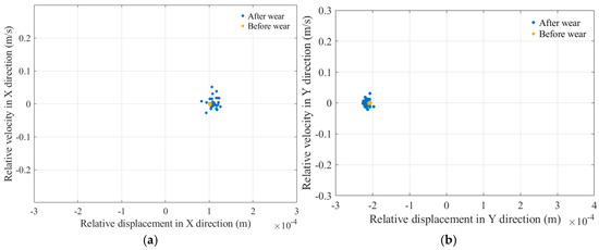
Figure 18.
Poincaré map. (a) Poincaré map of clearance in X direction; (b) Poincaré map of clearance in Y direction.
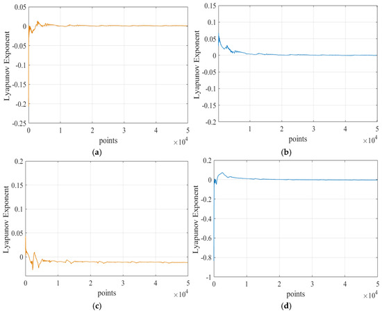
Figure 19.
Maximum Lyapunov exponent. (a) MLE in X direction before wear; (b) MLE in X direction after wear; (c) MLE in Y direction before wear; (d) MLE in Y direction after wear.
Table 4.
Parameter values for nonlinear characteristic evaluation.
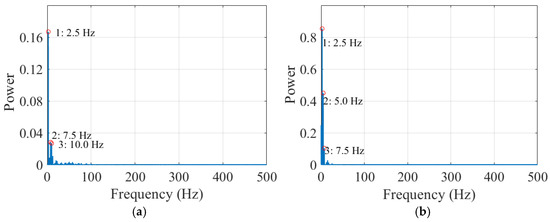
Figure 20.
Power density spectrum. (a) X direction after wear; (b) Y direction after wear.
5.4. Influence of Different Clearance Sizes on Dynamics
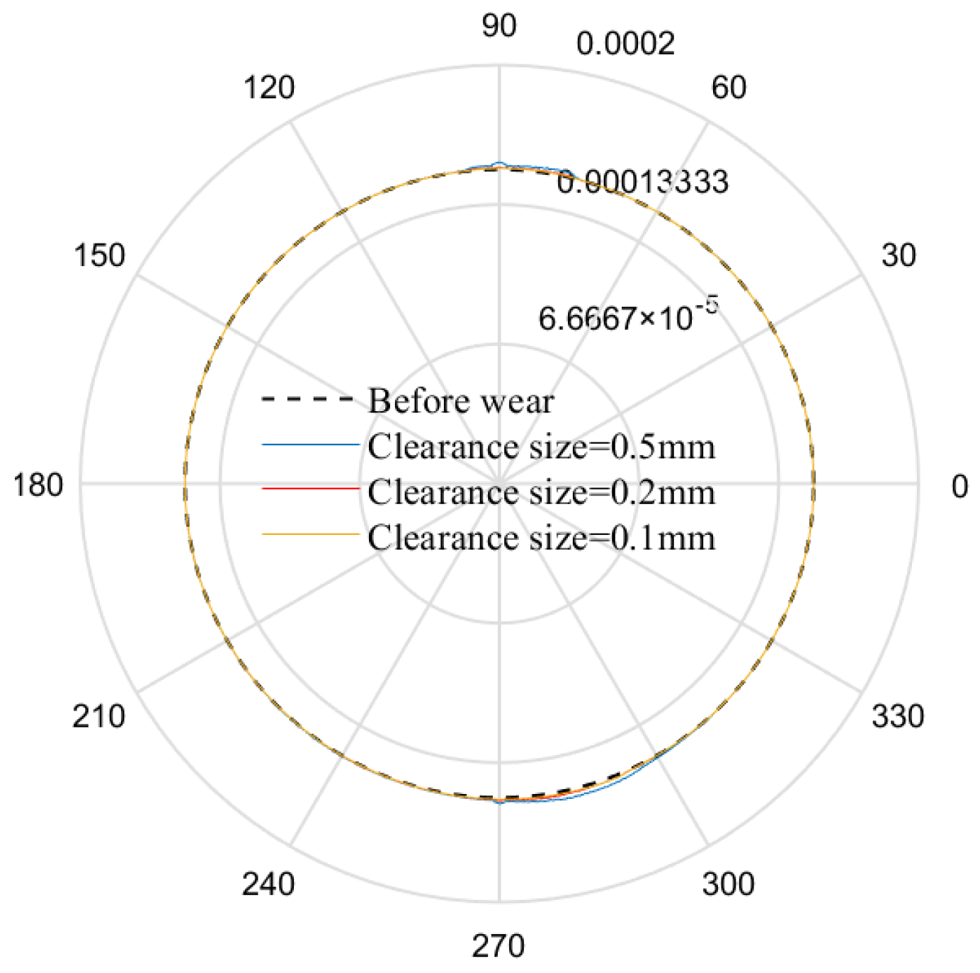
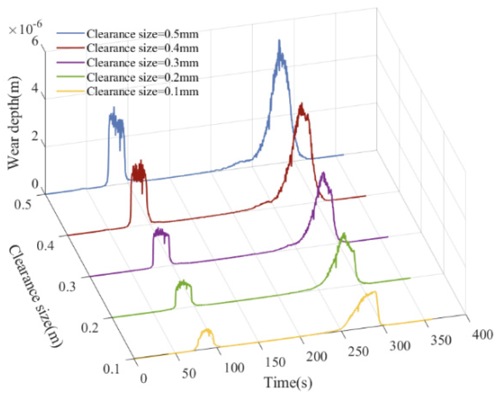
This section investigates the effects of clearance values on the mechanism, with the selection of 0.1 mm, 0.2 mm, and 0.5 mm, respectively, and the driving speed of the selected mechanism is 2π rad/s. Based upon wear depth obtained from the operating mechanism for 100 cycles, we increased it by 10,000 times to approximate the wear depth obtained from the operating mechanism for 1 million cycles. The wear depth and reconstructed bearing surface corresponding to various clearance values are displayed in Figure 21 and Figure 22. It was found that the wear was mainly concentrated in two areas, and the wear depth increased with the increase in clearance value. The maximum wear depths corresponding to the initial clearance sizes of 0.1 mm, 0.2 mm, and 0.5 mm were 5.179 × 10⁻⁶ m, 2.29 × 10⁻⁶ m, and 1.501 × 10⁻⁶ m, respectively. It can be observed that as the clearance value increases, the distribution range of the worn surface profile expands to some extent, particularly within the interval of [202°, 325°]. Furthermore, the deterioration of the surface profile of the kinematic pair does not follow a linear trend but exhibits a nonlinear intensification pattern.
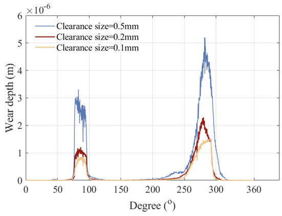
Figure 21.
Wear depth.
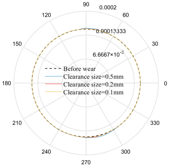
Figure 22.
Reconstruction of bearing surface.
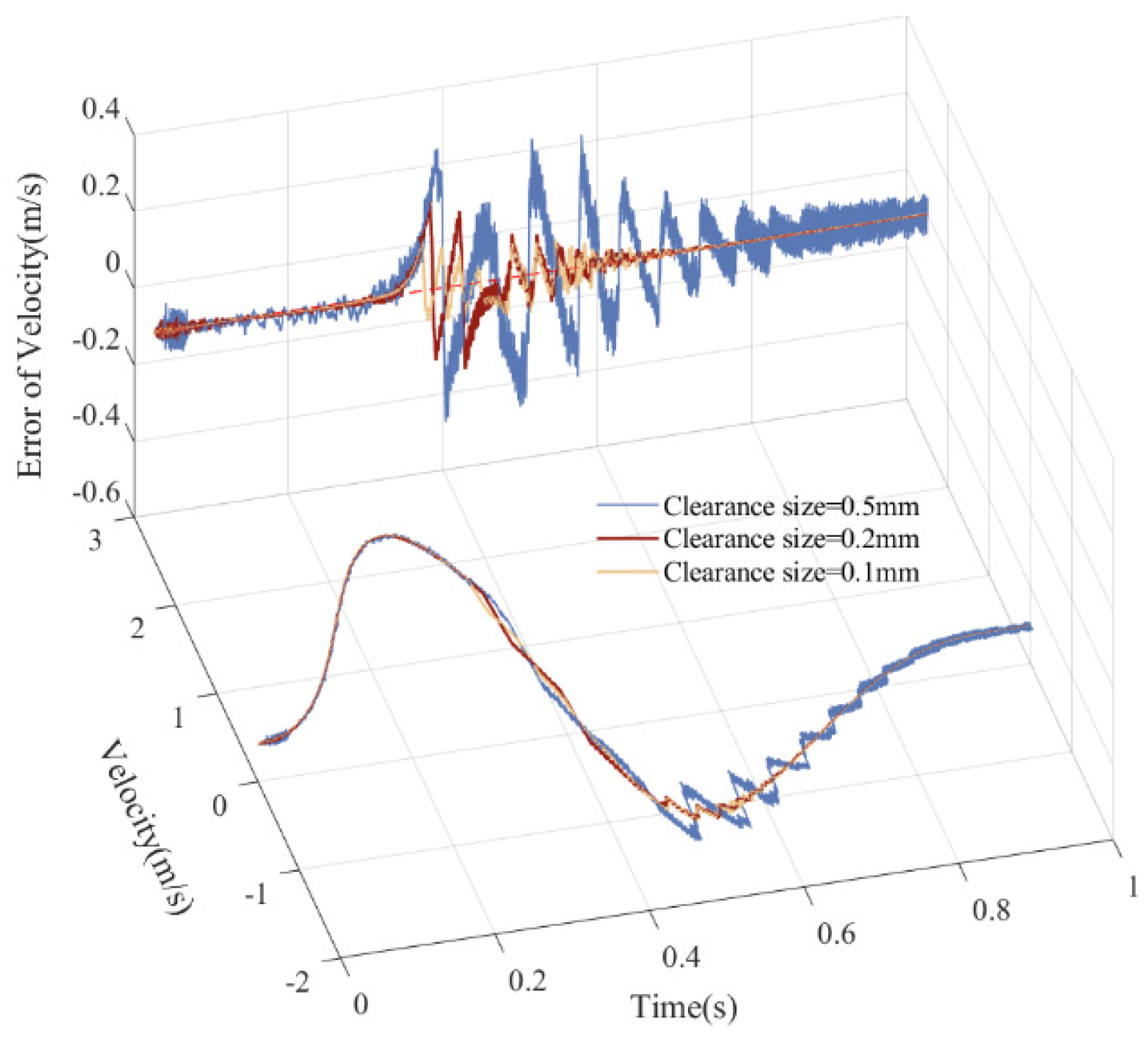
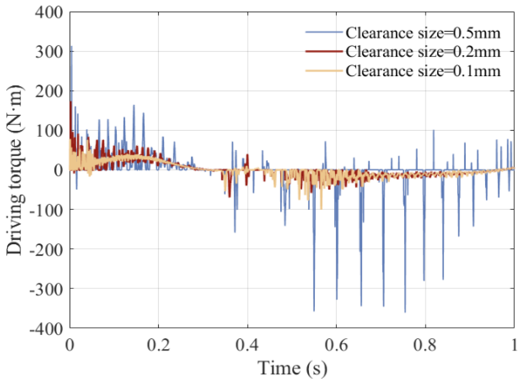
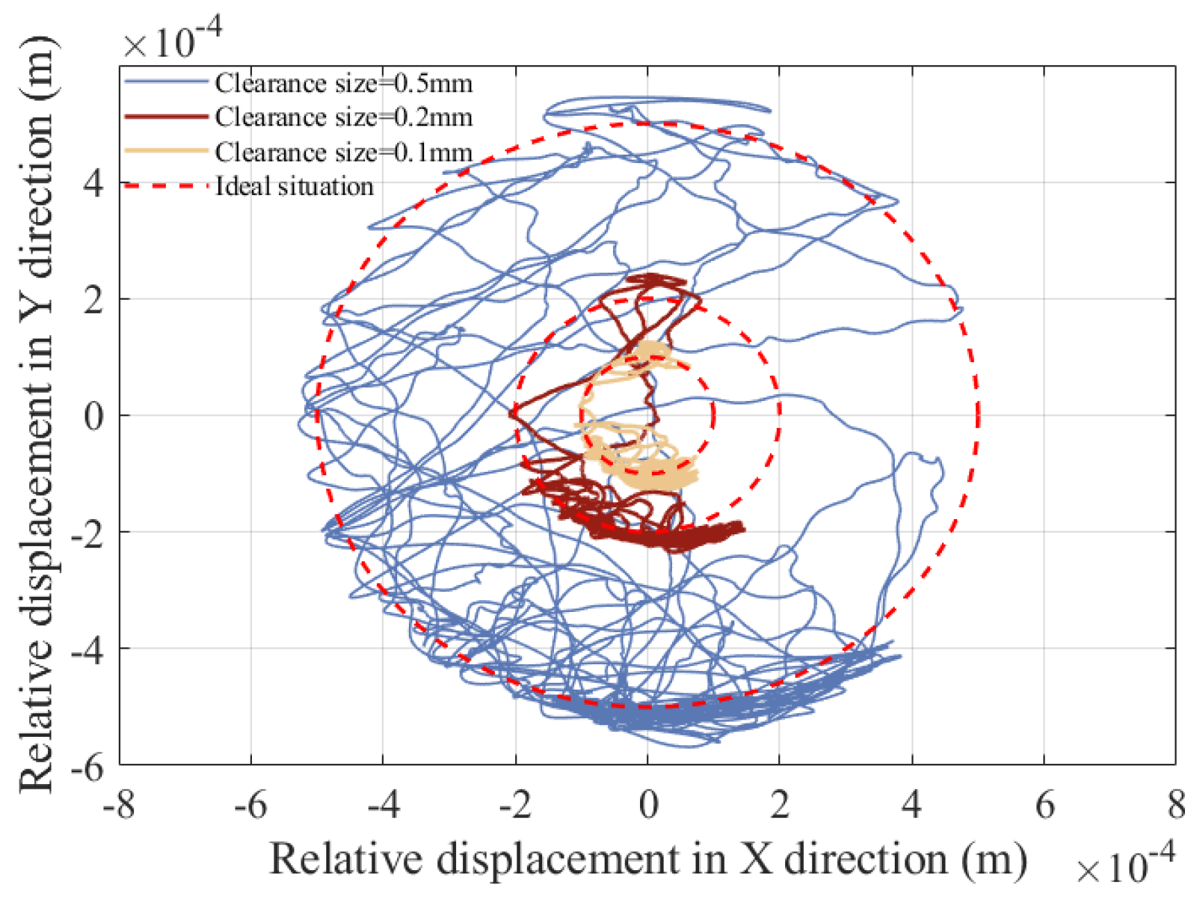
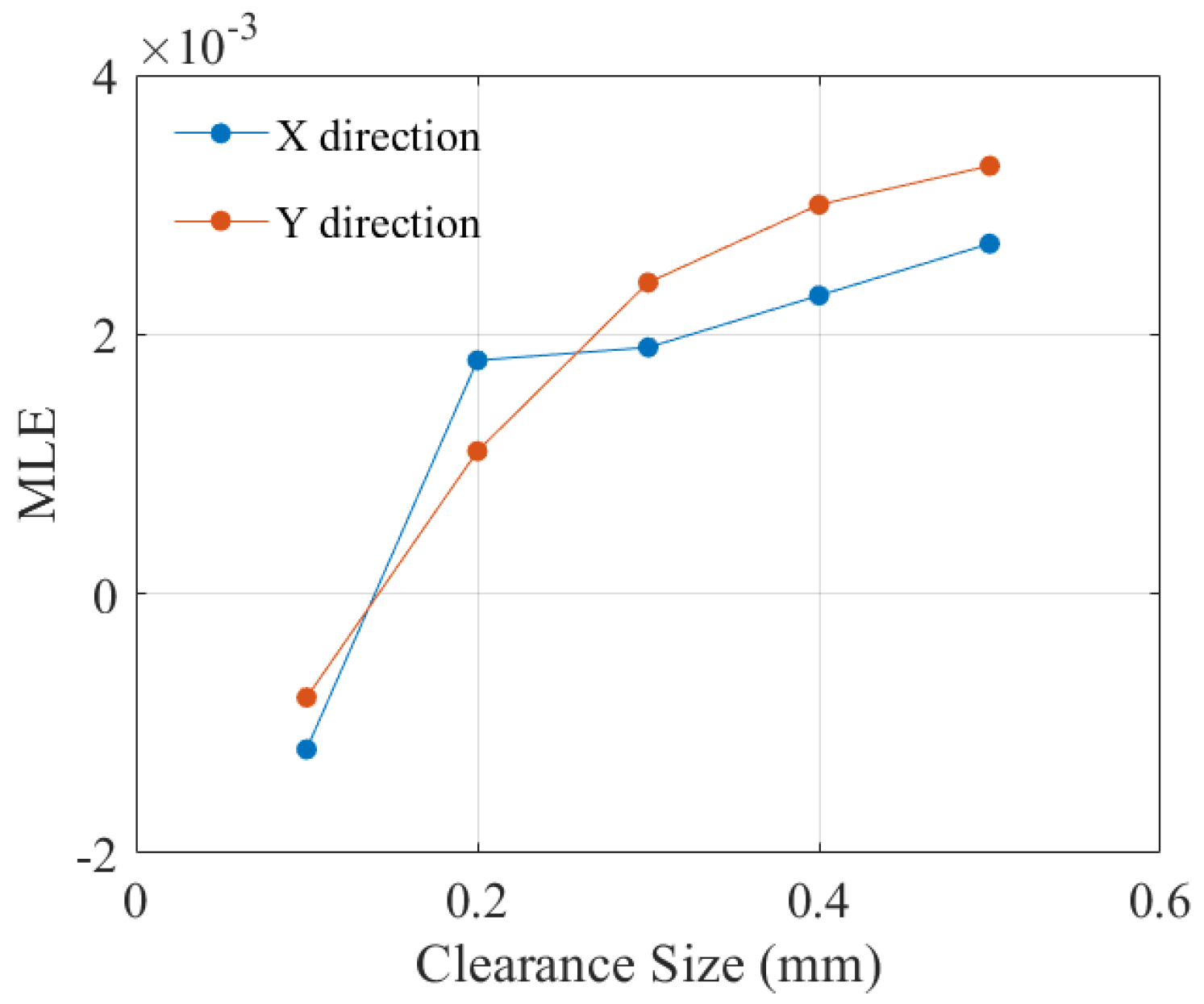
Based on the worn surface of the pair, the motion characteristics and dynamic response are solved and analyzed separately. Figure 23 and Figure 24 show the motion characteristics, including displacement, displacement error, velocity, and velocity error. It was found that clearance size has a relatively small impact on displacement, and the sensitivity of speed to the size of clearance is greater than displacement. As clearance size increases, displacement error and velocity error also increase. As displayed in Figure 25 and Figure 26, contact force, embedding depth, and driving torque indicate that, as the clearance value increases, the embedding depth of the shaft in bearing also increases, leading to an increase in the maximum size of collision force response. As the magnitude of collision force at the clearance directly affects the motion state of the driving component, this leads to an increase in the maximum value of driving torque. The strain curves of rod 3 and rod 4 vary with the clearance value are shown in Figure 27. As clearance size increases, collision force at clearance increases, which further increases the deformation of the flexible rod. And as shown in Figure 28, as clearance value increases, the movement trajectory of the shaft becomes more chaotic, and the depth of the shaft’s insertion into the bearing also increases. The maximum values of each dynamic response are displayed in Table 5. The main reason for the above is that the larger the clearance value, the greater the collision force at the clearance pair, which increases the wear depth of the moving pair, leading to an acceleration of the vibration frequency of the response curve and an increase in the response peak. As shown in Figure 29, the increase in clearance value deepens the wear depth at the joint containing clearance motion, which excites high-frequency vibrations, accelerating the rise in frequency and peak values of the response curves, and ultimately leading to a decline in the stability of the mechanism. As shown in Figure 30, with the increase in clearance size, the MLE for both the X and Y directions rise, indicating an increase in the degree of chaos within the system. The MLE for the X direction increases more slowly when the clearance size is greater than 0.2 mm, with a maximum value of 0.0027.
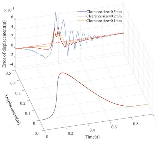
Figure 23.
Displacement and displacement error.
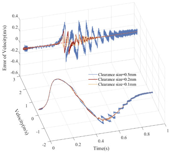
Figure 24.
Speed and speed error.

Figure 25.
Contact force and embedding depth after wear.
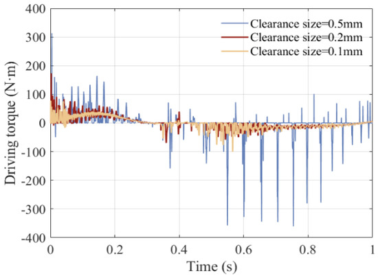
Figure 26.
Driving torque.
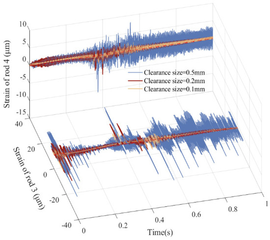
Figure 27.
Strain of flexible members.

Figure 28.
Central trajectory.
Table 5.
Maximum value of dynamic with different clearance size.
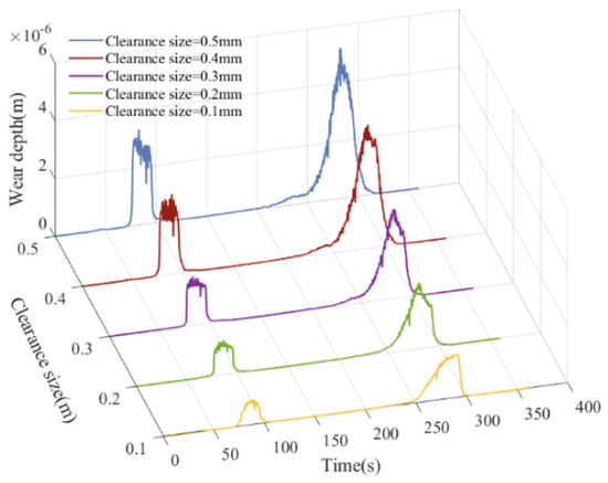
Figure 29.
Wear depth with increasing clearance value.
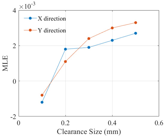
Figure 30.
MLE with increasing clearance value.
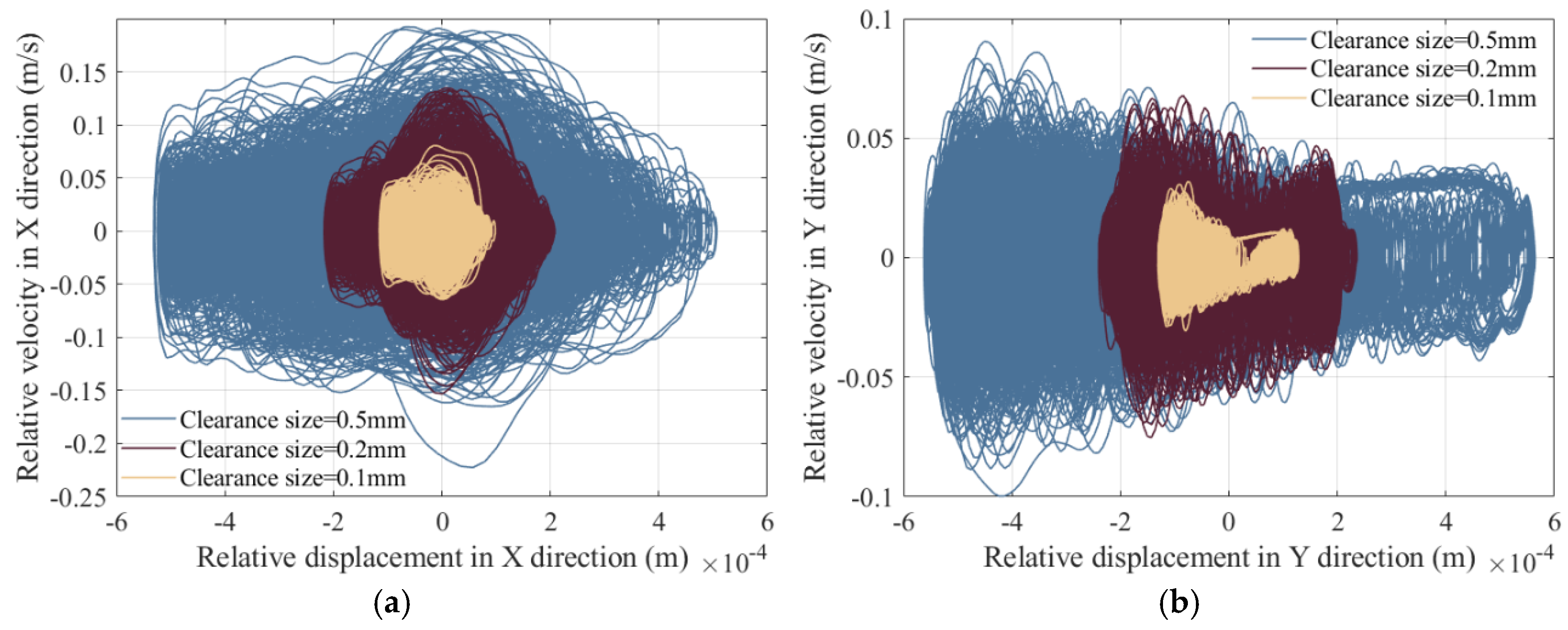
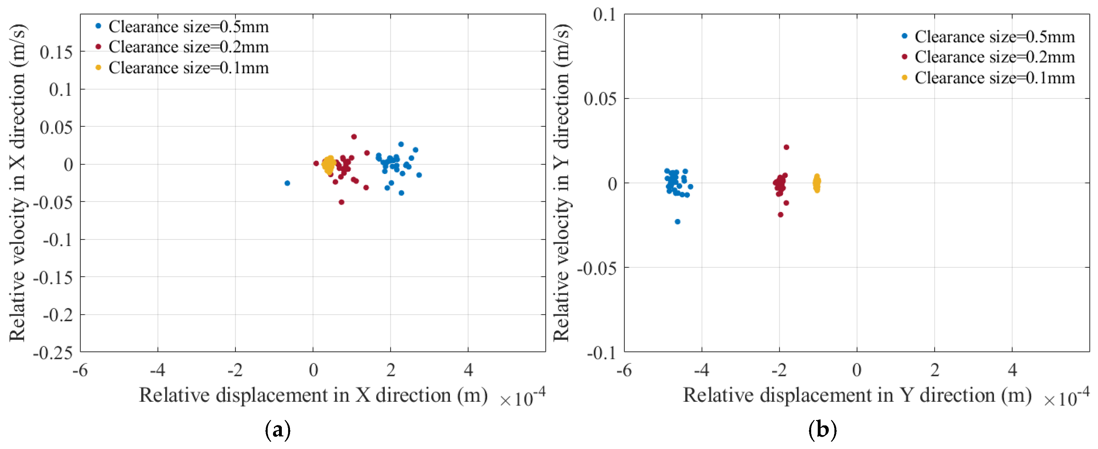
Phase diagram and Poincaré mapping diagram displayed in Figure 31 and Figure 32 are used to research the effects of three various clearance sizes on motion state at clearance, which are 0.1 mm, 0.2 mm, and 0.5 mm, respectively. The distribution area of the phase trajectory lines in the phase diagram and the discrete area of mapping points in the Poincaré map show that, as clearance size increases, embedding depth at clearance deepens, leading to an increase in collision force at clearance, thereby making the motion state of the shaft in the bearing more chaotic.

Figure 31.
Phase diagram. (a) Phase diagram of clearance in X direction; (b) Phase diagram of clearance in Y direction.
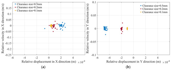
Figure 32.
Poincaré map. (a) Poincaré map of clearance in X direction; (b) Poincaré map of clearance in Y direction.
5.5. Influence of Various Driving Velocities on Dynamics
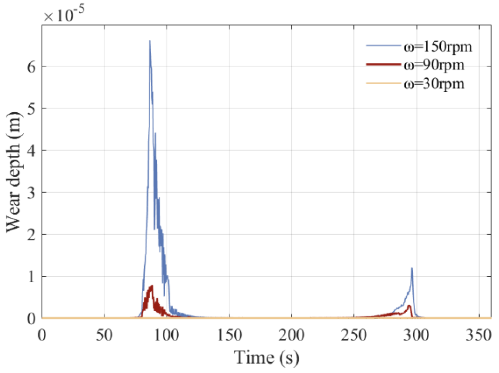
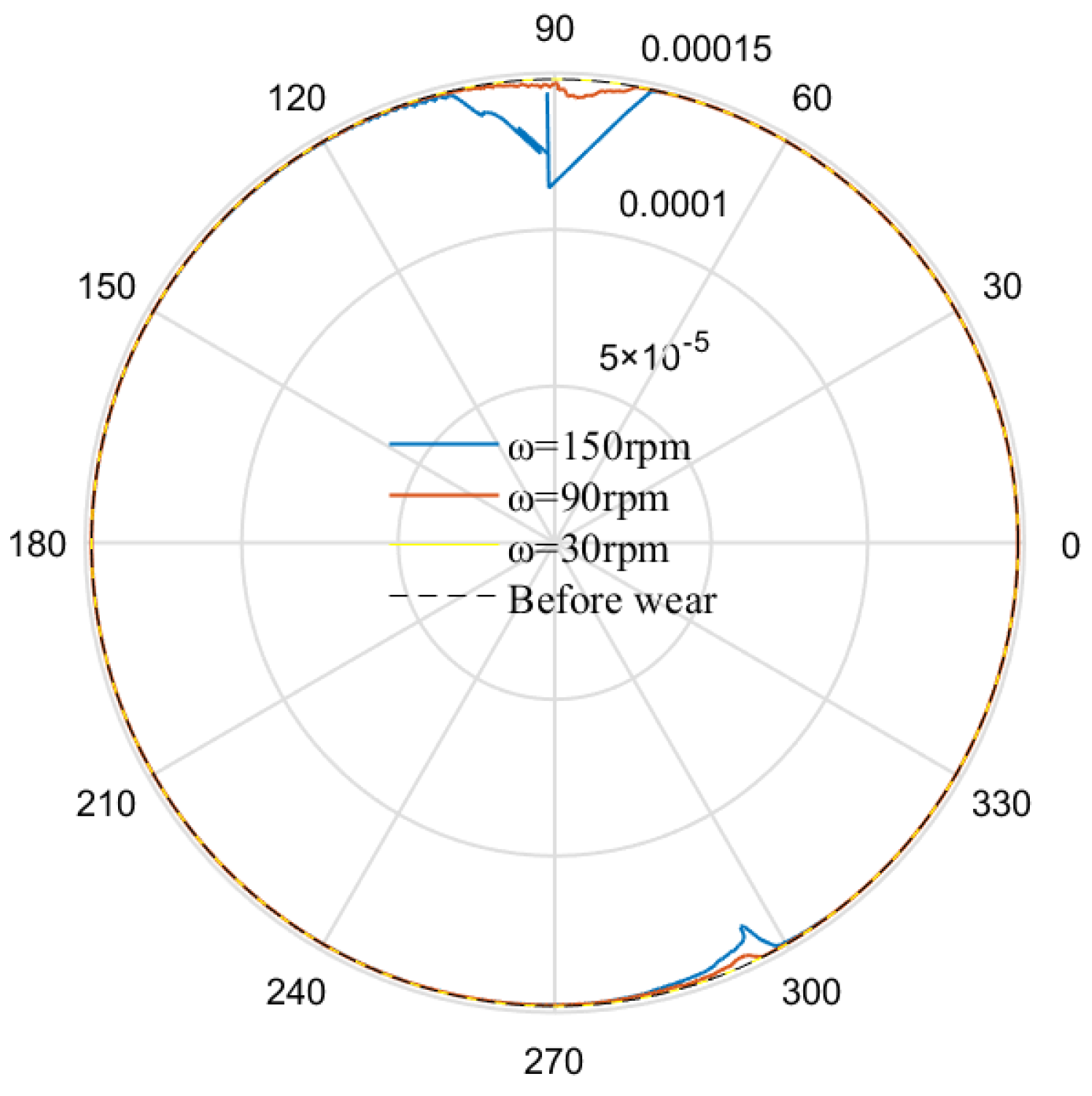
This section investigates the influence of different driving speeds on wear characteristics and nonlinear dynamics, with driving speeds selected as 30 rpm, 90 rpm, and 150 rpm, respectively. The selected clearance value at clearance pair is 0.2 mm. Based upon the wear depth obtained from operating the mechanism for 100 cycles, we increased it by 10,000 times to approximate the wear depth obtained from operating the mechanism for 1 million cycles. The wear depth and shaft surface reconstruction maps corresponding to three various driving speeds are displayed in Figure 33 and Figure 34. The visible wear area is mainly concentrated in two areas, mainly because the main collision of the shaft in the bearing is concentrated in these two areas, and as driving speed increases, wear depth increases and the wear area expands. The maximum wear depths corresponding to driving speeds of 30 rpm, 90 rpm, and 150 rpm are 8.59 × 10⁻⁸ m, 7.884 × 10⁻⁶ m, and 6.617 × 10⁻⁵ m, respectively. This wear pattern indicates that the local contact stress concentration effect becomes more pronounced under high-speed operation, leading to nonlinear growth in wear depth and area. Furthermore, the evolution of the clearance surface profile further reveals the cumulative effect of wear: as the driving speed increases, surface roughness rises, and the non-uniformity of the microscopic morphology intensifies, thereby accelerating the expansion and deterioration of wear.

Figure 33.
Wear depth.
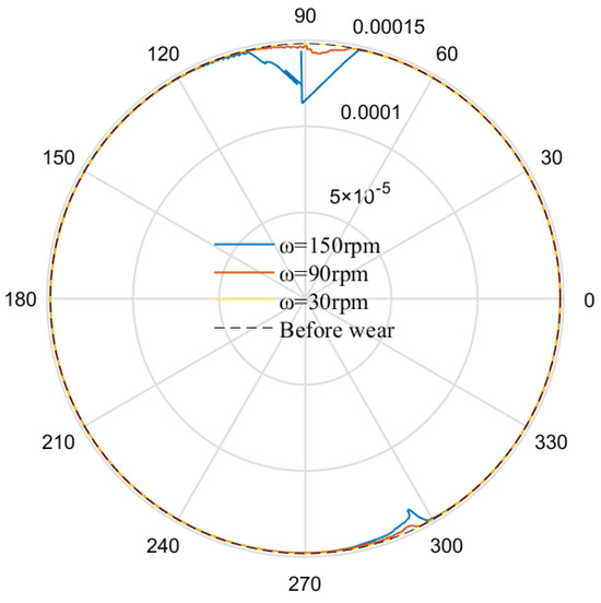
Figure 34.
Reconstruction of shaft surface.
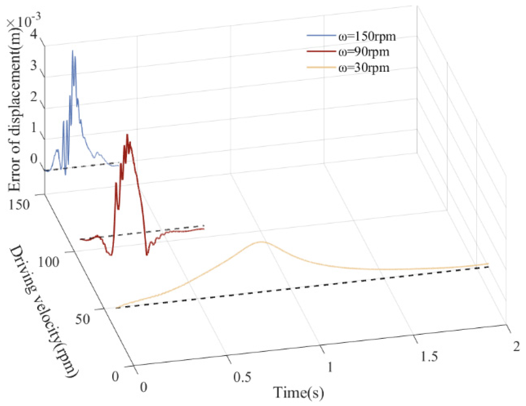
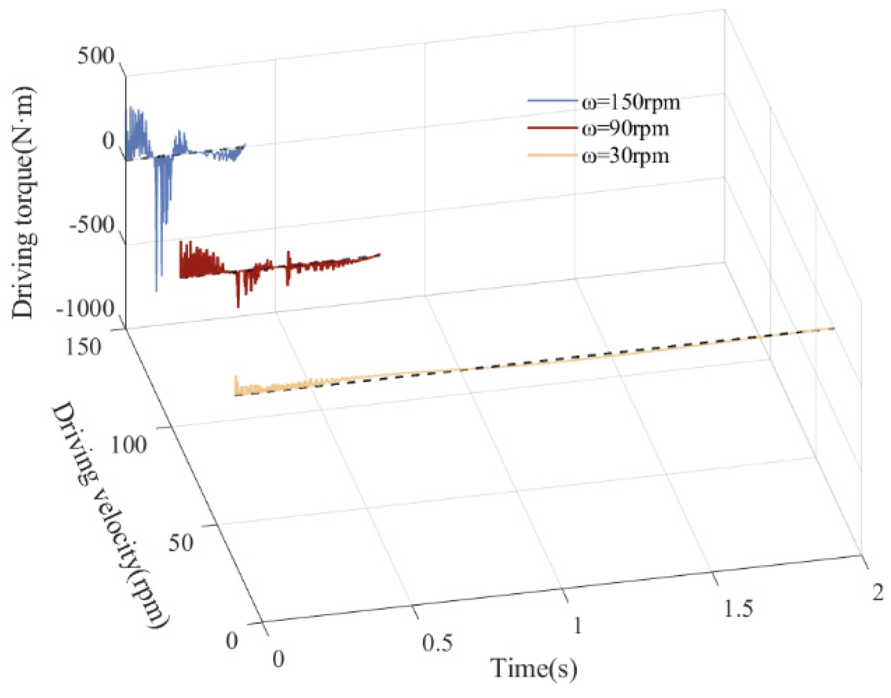
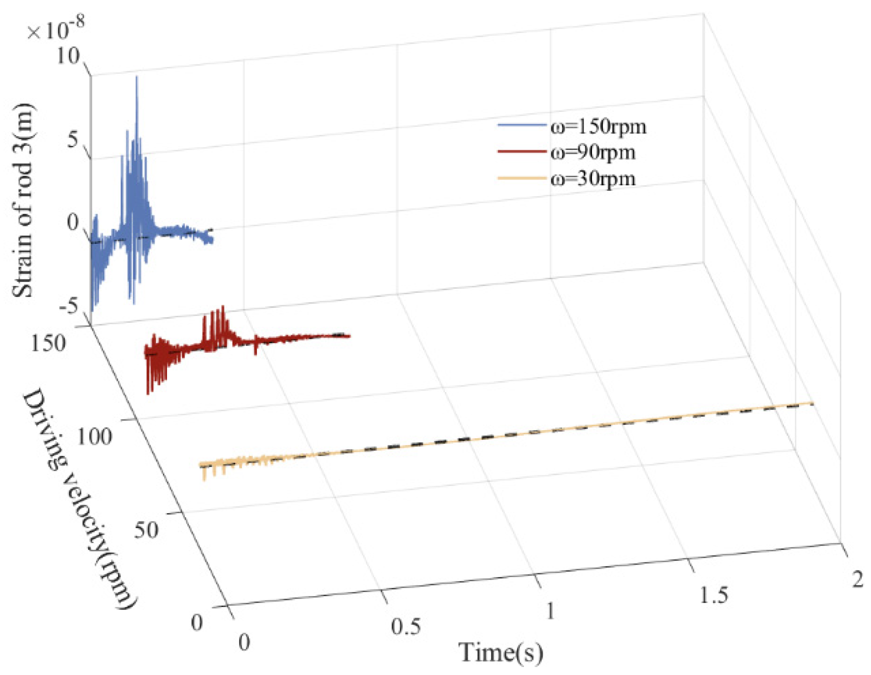
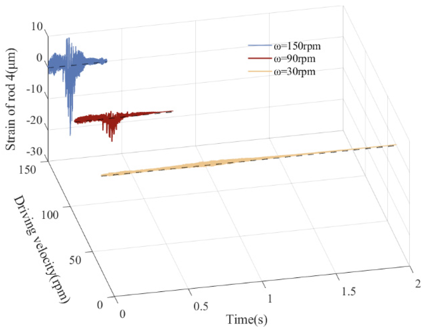
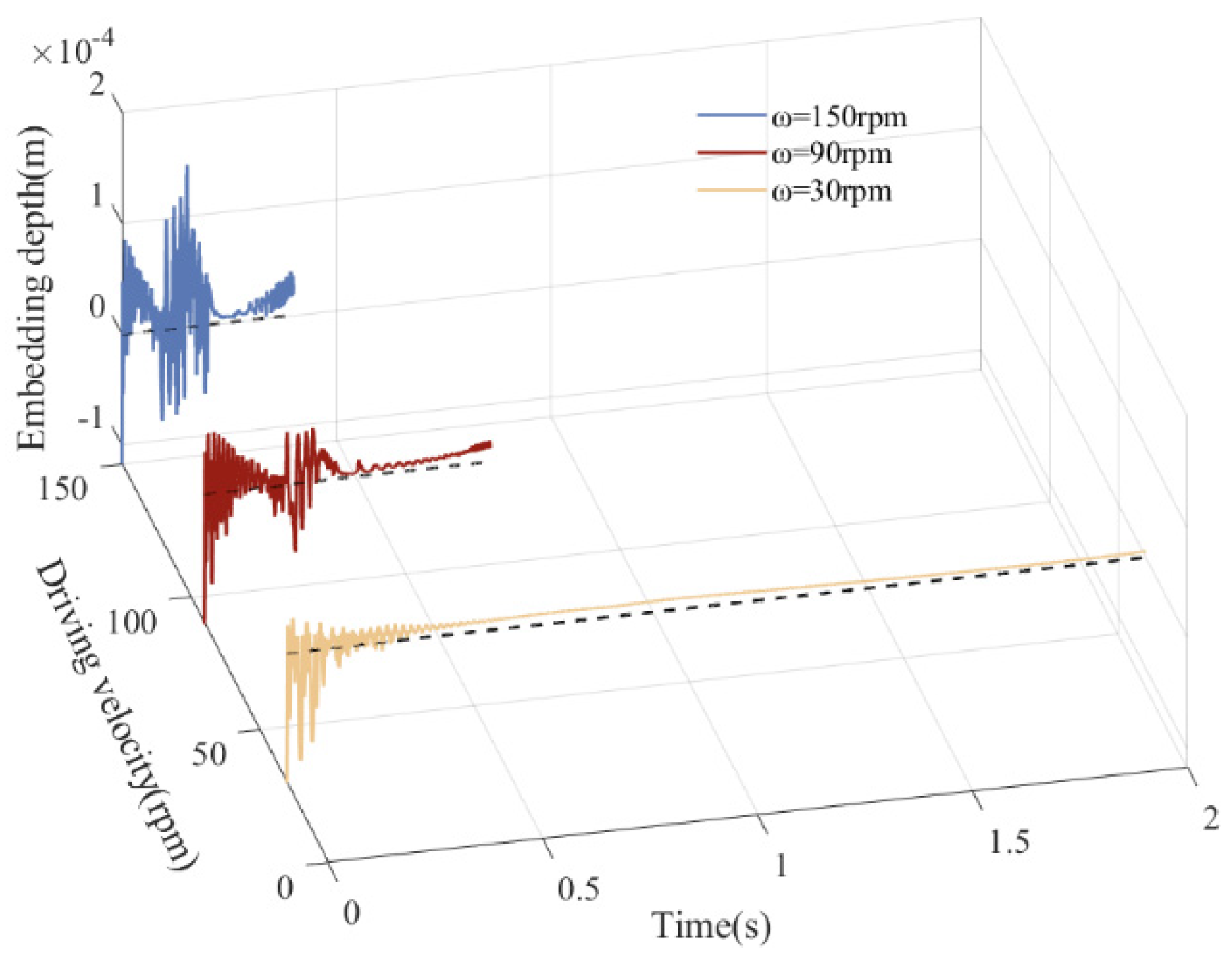
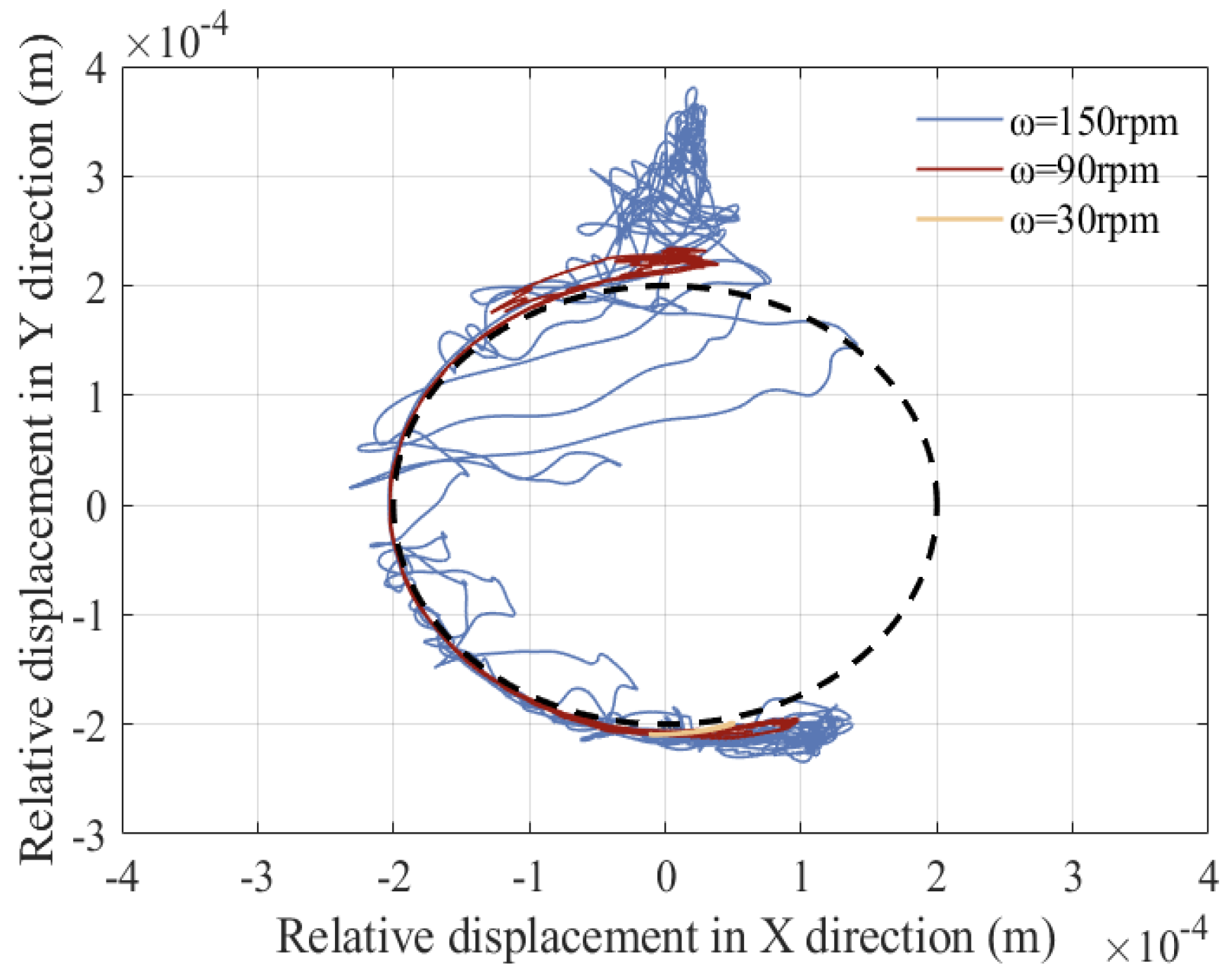
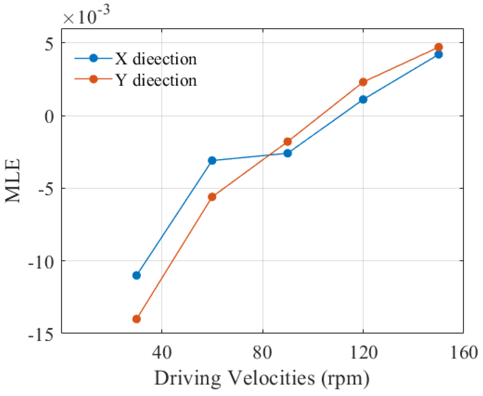
As shown in Figure 35, Figure 36, Figure 37, Figure 38, Figure 39, Figure 40, Figure 41 and Figure 42, the displacement error, velocity error, collision force, driving torque, strain of component 3, strain of component 4, embedding depth at clearance joint, and center trajectory at clearance correspond to the driving speed increasing from 30 rpm to 90 rpm and 150 rpm, respectively. As the driving speed increases, collision in the clearance motion pair intensifies, leading to a deeper embedding depth. Ultimately, peak dynamic response increases (including displacement error, velocity error, collision force, driving force moment, strain of component 3, and strain of component 4). Simultaneously, the motion trajectory of the shaft within the bearing becomes more chaotic, indicating a transition from periodic to chaotic motion. Maximum values of dynamic response under various driving speeds are displayed in Table 6. The trend of wear depth at clearance with a variation in driving speed is displayed in Figure 43. This trend reflects the intensification of local contact stress concentration under high-speed operation and the positive feedback mechanism between wear and dynamic response, where an increase in driving speed leads to enhanced collision forces, which in turn deepen wear, further worsen dynamic responses, and ultimately reduce system stability. As shown in Figure 44, similar to the case with constant clearance, the MLE for both the X and Y directions increase with the driving velocity. However, the rate of increase slows down beyond 60 rpm, with the highest MLE values for the X and Y directions being 0.0042 and 0.0047, respectively.
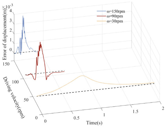
Figure 35.
Displacement error.
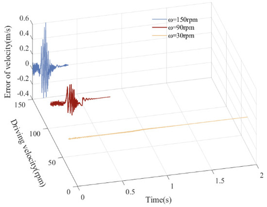
Figure 36.
Velocity error.
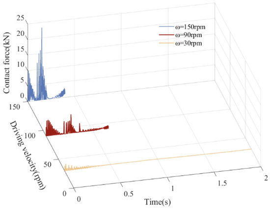
Figure 37.
Contact force.
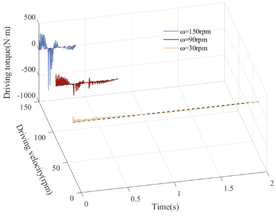
Figure 38.
Driving torque.

Figure 39.
Strain of flexible member 3.
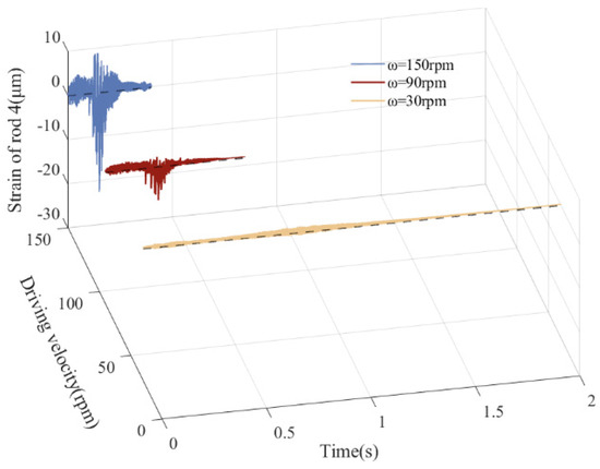
Figure 40.
Strain of flexible member 4.
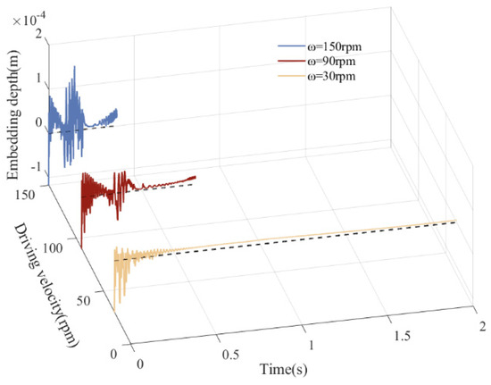
Figure 41.
Embedding depth.
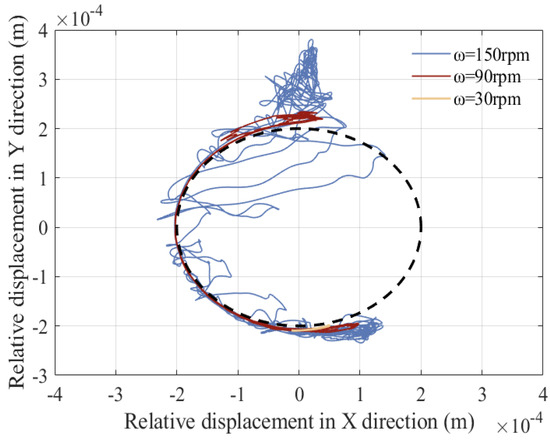
Figure 42.
Central trajectory.
Table 6.
Maximum value of dynamic with different driving speed.
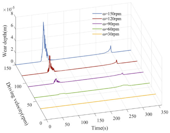
Figure 43.
Wear depth with increasing driving velocity.
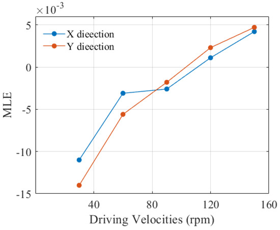
Figure 44.
MLE with increasing driving velocity.
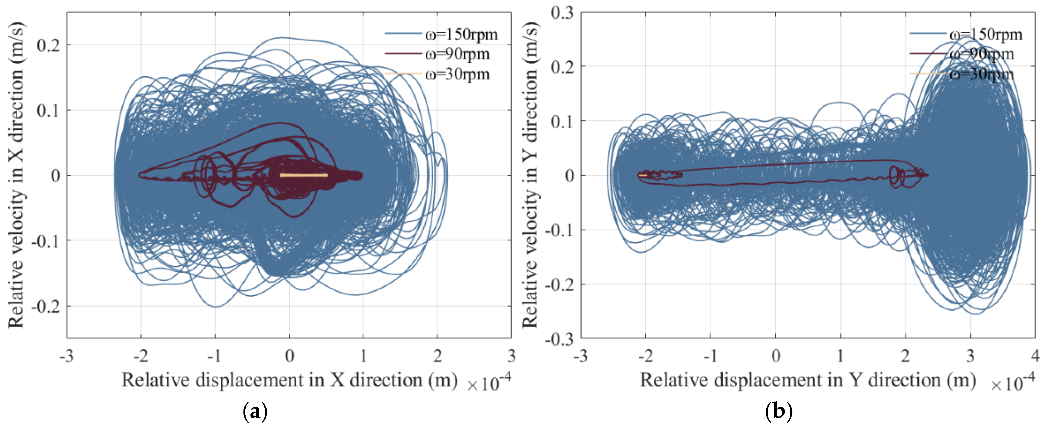
As shown in Figure 45 and Figure 46, the phase diagram and Poincaré mapping diagram of motion pairs with variations in driving speed of 30 rpm, 90 rpm, and 150 rpm, respectively. As driving speed increases, the distribution area and degree of disorder of the phase trajectory at the clearance joint strengthen, and the distribution range of mapping points becomes larger and more chaotic.
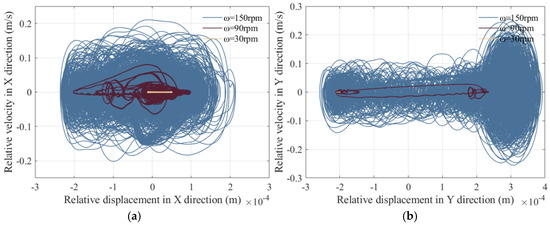
Figure 45.
Phase diagram. (a) Phase diagram of clearance in X direction; (b) Phase diagram of clearance in Y direction.
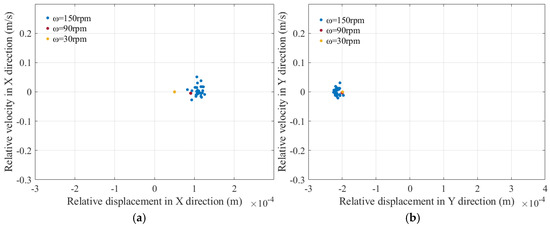
Figure 46.
Poincaré map. (a) Poincaré map of clearance in X direction; (b) Poincaré map of clearance in Y direction.
6. Conclusions
To investigate the wear characteristics of clearance joints, the Archard wear theory was integrated into the dynamic framework of multi-link mechanisms with clearance joints. Building upon this foundation, a comprehensive dynamic model for flexible multi-link mechanisms was established, incorporating the effects of irregular wear patterns and flexible rod dynamics. This model enables a detailed analysis of the nonlinear behavior of the system. The specific research framework comprises the following components:
- (1)
- A 2D beam element model was developed using the ANCF, integrating the Archard wear model to characterize irregular wear patterns, thereby establishing a flexible multibody dynamics framework for multi-link mechanisms with clearance joints. This framework enables systematic chaos identification and nonlinear dynamic analysis.
- (2)
- A comparative analysis of before and after wear dynamic responses revealed localized wear concentration in the [75°, 132°] and [252°, 310°] intervals of kinematic pairs, attributed to stress concentration and dynamic load redistribution. After wear, the maximum contact force amplitude of the joint increased by 1.54 times.
- (3)
- This study investigated the nonlinear effects of wear-induced clearances in rigid–flexible coupled systems under varying operational conditions. The results indicate that enlarged clearances accelerate the transition from periodic to chaotic motion due to intensified wear. System dynamics exhibit higher sensitivity to driving speed variations than clearance size, with rotational speeds below 90 rpm effectively suppressing wear severity and stabilizing motion.
Author Contributions
Conceptualization, Y.J. and S.J.; methodology, Y.J.; software, K.M.; validation, J.K.; formal analysis, J.K.; investigation, Y.J. and S.J.; resources, S.J.; data curation, K.M.; writing—original draft preparation, Y.J.; writing—review and editing, Y.J. and S.J.; visualization, K.M.; supervision, S.J.; project administration, Y.J.; funding acquisition, S.J. All authors have read and agreed to the published version of the manuscript.
Funding
This research was funded by Natural Science Foundation of Shandong Province grant number ZR2023QE039, Open Project of Key Laboratory of Special Motors and High Voltage Electrical Appliances, Ministry of Education grant number KFKT202402. And the APC was funded by Shuai Jiang.
Data Availability Statement
The results of this research are supported by data included within this paper.
Conflicts of Interest
The authors ascertain there are no conflicting interests to declare.
Nomenclature
| a | contact half width |
| Aw | contact area |
| c | clearance joint value |
| ce | material’s recovery coefficient |
| cd | dynamic correction coefficient |
| cf | coefficient of friction |
| clearance size at discrete region n | |
| D | hysteresis damping factor |
| hysteresis damping factor after wear | |
| e | eccentricity vector |
| ef | absolute node coordinates |
| E1, E2 | elastic modulus of the bearing and shaft |
| E* | Young’s modulus |
| Fe | elastic force of a flexible beam element |
| Ff | elastic force of flexible components |
| Fn | contact force |
| contact force at clearance joint after wear | |
| friction force at clearance joint after wear | |
| h | wear depth |
| hn | wear depth within discrete area code |
| k | wear coefficient |
| stiffness coefficient | |
| Kl | compressive stiffness of the unit |
| Kt | bending stiffness of the unit |
| stiffness coefficient after wear | |
| l | unit length |
| L | axial contact length of hinge |
| M | total number of iterations in the calculation of Lyapunov exponent |
| Me | mass matrix of elastic beam elements |
| Mr | mass matrix of the rigid components |
| Mf | mass matrix of flexible components |
| q | generalized coordinates of entire system |
| qf | generalized coordinate of flexible components |
| qr | generalized coordinate of the system’s rigid components |
| Qe | generalized force of the flexible beam element |
| Qf | total external force of flexible components |
| Qr | total external force of the rigid components |
| contact points | |
| r | absolute position vector of any point on element |
| position vectors of contact points | |
| curvature radius at the discrete region n of the bearing and shaft | |
| s | slip distance |
| S | shape function |
| v0, v1 | speed limit value |
| V | wear volume |
| x | local coordinate of any point before deformation |
| X(ti) | time series |
| Y(ti) | time series reconstructed from phase space |
| parameter of Baumgarte stabilization algorithm | |
| parameter of Baumgarte stabilization algorithm | |
| right side of acceleration constraint equations | |
| δ | penetration depth |
| relative normal contact velocity, | |
| elative embedding depth at the discrete region n | |
| l | strain of unit |
| Lagrange multiplier | |
| right side of velocity constraint equations | |
| υ1, υ2 | Poisson’s ratios of bearing and shaft |
| maximum Lyapunov exponent | |
| Φ | constraint equation of mechanism |
| Φq | Jacobian matrix of constraint equation |
| Φqr | derivative of constraint equation with respect to generalized coordinates of rigid components |
| Φqf | derivative of constraint equation with respect to generalized coordinates of flexible components |
| Φt | differentiation of the constraint equation with respect to time |
| ANCF | Absolute Nodal Coordinate Formulation |
| L-N | Lankarani and Nikravesh |
| MLE | maximum Lyapunov exponent |
References
- Millan, P.; Pagaimo, J.; Magalhães, H.; Ambrósio, J. Clearance joints and friction models for the modelling of friction damped railway freight vehicles. Multibody Syst. Dyn. 2023, 58, 21–45. [Google Scholar] [CrossRef]
- Li, Y.; Li, M.; Liu, Y.; Geng, X.; Cui, C. Parameter optimization for torsion spring of deployable solar array system with multiple clearance joints considering rigid-flexible coupling dynamics. Chin. J. Aeronaut. 2022, 35, 509–524. [Google Scholar] [CrossRef]
- Xu, L.; Han, Y.; Dong, Q.; Jia, H. An approach for modelling a clearance revolute joint with a constantly updating wear profile in a multibody system: Simulation and experiment. Multibody Syst. Dyn. 2019, 45, 457–478. [Google Scholar] [CrossRef]
- Korayem, M.H.; Ghariblu, H. Analysis of Wheeled Mobile Flexible Manipulator Dynamic Motions with Maximum Load Carrying Capacitie. Robot. Auton. Syst. 2004, 48, 63–76. [Google Scholar] [CrossRef]
- Bai, Z.; Ning, Z.; Zhou, J. Study on Wear Characteristics of Revolute Clearance Joints in Mechanical Systems. Micromachines 2022, 13, 1018. [Google Scholar] [CrossRef]
- Wang, G.; Liu, H. Three-Dimensional Wear Prediction of Four-Degrees-of-Freedom Parallel Mechanism with Clearance Spherical Joint and Flexible Moving Platform. J. Tribol. 2018, 140, 031611. [Google Scholar] [CrossRef]
- Chaturvedi, E.; Sandu, C.; Sandu, A. A nonsmooth dynamics framework for simulating frictionless spatial joints with clearances. Multibody Syst. Dyn. 2024, 63, 3–37. [Google Scholar] [CrossRef]
- Wang, C.; Le, T.D.; Huynh, N.T. Optimal rigid-flexible dynamic of space slider-crank mechanism with clearance joints. Sādhanā 2023, 48, 44. [Google Scholar] [CrossRef]
- Cirelli, M.; Autiero, M.; Belfiore, N.P.; Paoli, G.; Pennestrì, E.; Valentini, P.P. Review and comparison of empirical friction coefficient formulation for multibody dynamics of lubricated slotted joints. Multibody Syst. Dyn. 2024, 63, 83–104. [Google Scholar] [CrossRef]
- Guo, J.; Wang, Y.; Zhang, X.; Cao, S.; Liu, Z. Dynamic characteristic of rudder loop with rough revolute joint clearance. Nonlinear Dyn. 2024, 112, 3179–3194. [Google Scholar] [CrossRef]
- Bai, Z.; Liu, T.; Li, J.; Zhao, J. Numerical and experimental study on dynamic characteristics of planar mechanism with mixed clearances. Mech. Based Des. Struct. Mach. 2023, 51, 6142–6165. [Google Scholar] [CrossRef]
- Zhang, S.; Gao, Y.; Yang, J. Dynamic modeling and analysis of vehicle scissor door mechanism with mixed clearance based on a hybrid contact force model. Multibody Syst. Dyn. 2024, 61, 509–538. [Google Scholar] [CrossRef]
- Chouaibi, Y.; Chebbi, A.H.; Affi, Z.; Romdhane, L. Precision comparison of two 3-DoF translational parallel manipulators based on the orientation errors due to joint clearances. Robotica 2022, 40, 3751–3767. [Google Scholar] [CrossRef]
- Korayem, M.H.; Ghariblu, H.; Basu, A. Dynamic Load Carrying Capacity of Mobile-Base Flexible Joint Manipulators. Int. J. Adv. Manuf. Technol. 2005, 25, 62–70. [Google Scholar] [CrossRef]
- Song, N.; Peng, H.; Kan, Z. Nonsmooth strategy for rigid-flexible multibody system considering different types of clearance joints and lubrication. Multibody Syst. Dyn. 2022, 55, 341–374. [Google Scholar] [CrossRef]
- Wang, Z.; Jin, G.; Liang, D.; Wei, Z.; Chang, B.; Zhou, Y. Nonlinear analysis of complex mechanisms with multi-clearances considering dry friction and lubricated joints. Nonlinear Dyn. 2023, 111, 10911–10938. [Google Scholar] [CrossRef]
- Jiang, J.; Yang, W.; Wei, H.; Peng, B. Distribution Analysis of Multiple Limit Cycles of Vehicle Shimmy System with Consideration of Joint Clearances. Mech. Solids 2022, 57, 1467–1474. [Google Scholar] [CrossRef]
- Wu, X.; Sun, Y.; Wang, Y.; Chen, Y. Passive chaos suppression for the planar slider-crank mechanism with a clearance joint by attached vibro-impact oscillator. Mech. Mach. Theory 2022, 174, 104882. [Google Scholar] [CrossRef]
- Yang, L.; Li, J.; Zhou, X.; Jiang, C. Optimized trajectory tracking control of the clearance manipulator based on improved PSO algorithm. Proc. Inst. Mech. Eng. Part C J. Mech. Eng. Sci. 2022, 236, 6424–6439. [Google Scholar] [CrossRef]
- Cheng, Y.; Zhuang, X.; Yu, T. Time-dependent reliability analysis of planar mechanisms considering truncated random variables and joint clearances. Probabilistic Eng. Mech. 2024, 75, 103552. [Google Scholar] [CrossRef]
- Jiang, X.; Bai, Z. Dynamic analysis for mechanical system with clearance joint considering dependent interval parameters. Mech. Based Des. Struct. Mach. 2024, 52, 2726–2748. [Google Scholar] [CrossRef]
- Jia, Y.; Chen, X.; Zhang, L.; Ning, C. Dynamic characteristics and reliability analysis of parallel mechanism with clearance joints and parameter uncertainties. Meccanica 2023, 58, 813–842. [Google Scholar] [CrossRef]
- Bai, Z.; Zhao, Y.; Chen, J. Dynamics analysis of planar mechanical system considering revolute clearance joint wear. Tribol. Int. 2013, 64, 85–95. [Google Scholar] [CrossRef]
- Su, Y.; Chen, W.; Tong, Y.; Xie, Y. Wear prediction of clearance joint by integrating multi-body kinematics with finite-element method. Proc. Inst. Mech. Eng. Part J J. Eng. Tribol. 2010, 224, 815–823. [Google Scholar] [CrossRef]
- Zhuang, X.; Yu, T.; Sun, Z.; Song, K. Wear prediction of a mechanism with multiple joints based on ANFIS. Eng. Fail. Anal. 2021, 119, 104958. [Google Scholar] [CrossRef]
- Mukras, S.; Kim, N.H.; Mauntler, N.A.; Schmitz, T.L.; Sawyer, W.G. Analysis of planar multibody systems with revolute joint wear. Wear 2010, 268, 643–652. [Google Scholar] [CrossRef]
- López-Lombardero, M.; Cuadrado, J.; Cabello, M.; Martinez, F.; Dopico, D.; López-Varela, A. A multibody-dynamics based method for the estimation of wear evolution in the revolute joints of mechanisms that considers link flexibility. Mech. Mach. Theory 2024, 2024, 105583. [Google Scholar] [CrossRef]
- Wang, Z.; Jin, G.; Wei, Z.; Liang, D.; Chang, B.; Zhou, Y. Research on irregular wear mechanism of planar multi-body mechanical system with multi-clearance joints. Adv. Mech. Eng. 2022, 14, 1–16. [Google Scholar] [CrossRef]
- Ordiz, M.; Cuadrado, J.; Cabello, M.; Retolaza, I.; Martinez, F.; Dopico, D. Prediction of fatigue life in multibody systems considering the increase of dynamic loads due to wear in clearances. Mech. Mach. Theory 2021, 160, 104293. [Google Scholar] [CrossRef]
- Li, B.; Wang, M.; Gantes, C.J.; Tan, U.-X. Modeling and simulation for wear prediction in planar mechanical systems with multiple clearance joints. Nonlinear Dyn. 2022, 108, 887–910. [Google Scholar] [CrossRef]
- Jiang, D.; Han, Y.; Wang, K.; Jiang, S.; Cui, W.; Song, B. Functional degradation reliability analysis for non-uniform wear of multi-rotating joints of mechanical structures. Eng. Fail. Anal. 2024, 157, 107934. [Google Scholar] [CrossRef]
- Zhao, B.; Zhang, Z.; Dai, X. Modeling and prediction of wear at revolute clearance joints in flexible multibody systems. Proc. Inst. Mech. Eng. Part C J. Mech. Eng. Sci. 2014, 228, 317–329. [Google Scholar] [CrossRef]
- Gao, S.; Fan, S.W.; Fan, S. Optimization research on dynamic behavior for mechanism with clearance joint and wear. Proc. Inst. Mech. Eng. Part C J. Mech. Eng. Sci. 2024, 238, 6871–6891. [Google Scholar] [CrossRef]
- Zhuang, X.; Yu, T.; Liu, J.; Song, B. Kinematic reliability evaluation of high-precision planar mechanisms experiencing non-uniform wear in revolute joints. Mech. Syst. Signal Process. 2022, 169, 108748. [Google Scholar] [CrossRef]
- Zhuang, X. Time-dependent kinematic reliability of a dual-axis driving mechanism for satellite antenna considering non-uniform planar revolute joint clearance. Acta Astronaut. 2022, 197, 91–106. [Google Scholar] [CrossRef]
- Liu, J.; Xue, S.; Zhang, K.; Pang, H. Failure modeling and reliability analysis for motion mechanism with clearance joints under plastic deformation and wear. Eksploat. I Niezawodn. Maint. Reliab. 2023, 25, 169920. [Google Scholar] [CrossRef]
- Hou, Y.; Deng, Y.; Zeng, D. Dynamic modelling and properties analysis of 3RSR parallel mechanism considering spherical joint clearance and wear. J. Cent. South Univ. 2021, 28, 712–727. [Google Scholar] [CrossRef]
- Askari, E.; Flores, P. Coupling multi-body dynamics and fluid dynamics to model lubricated spherical joints. Arch. Appl. Mech. 2020, 90, 2091–2111. [Google Scholar] [CrossRef]
- Marques, F.; Isaac, F.; Dourado, N.; Flores, P. An enhanced formulation to model spatial revolute joints with radial and axial clearances. Mech. Mach. Theory 2017, 116, 123–144. [Google Scholar] [CrossRef]
- Jin, G.; Wang, Z.; Liang, D.; Wei, Z.; Chang, B.; Zhou, Y. Modeling and dynamics characteristics analysis of six-bar rocking feeding mechanism with lubricated clearance joint. Arch. Appl. Mech. 2023, 93, 2831–2854. [Google Scholar] [CrossRef]
- Lou, J.; Li, C. An improved model of contact collision investigation on multi-body systems with revolute clearance joints. Proc. Inst. Mech. Eng. Part D J. Automob. Eng. 2020, 234, 2103–2112. [Google Scholar] [CrossRef]
- Li, Y.; Yang, Y.; Li, M.; Liu, Y.; Huang, Y. Dynamics analysis and wear prediction of rigid-flexible coupling deployable solar array system with clearance joints considering solid lubrication. Mech. Syst. Signal Process. 2022, 162, 108059. [Google Scholar] [CrossRef]
- Erkaya, S.; Ibrahim, U. Modeling and simulation of joint clearance effects on mechanisms having rigid and flexible links. J. Mech. Sci. Technol. 2014, 28, 2979–2986. [Google Scholar] [CrossRef]
- Wolf, A.; Swift, J.B.; Swinney, H.L.; Vastano, J.A. Determining Lyapunov Exponents from a Time Series. Phys. D Nonlinear Phenom. 1985, 16, 285–317. [Google Scholar] [CrossRef]


Disclaimer/Publisher’s Note: The statements, opinions and data contained in all publications are solely those of the individual author(s) and contributor(s) and not of MDPI and/or the editor(s). MDPI and/or the editor(s) disclaim responsibility for any injury to people or property resulting from any ideas, methods, instructions or products referred to in the content. |
© 2025 by the authors. Licensee MDPI, Basel, Switzerland. This article is an open access article distributed under the terms and conditions of the Creative Commons Attribution (CC BY) license (https://creativecommons.org/licenses/by/4.0/).