Friction in Cylindrical Joints

Abstract

Cylindrical clearance joints are commonly employed in mechanisms that involve the rotation of a shaft spindle within a cylindrical sliding bearing. The intensity of the friction process in such joints is governed by several factors, including the clearance size between components, the materials of the interacting surfaces, the properties and characteristics of the lubricant, the surface roughness (asperities), and the magnitude of the relative velocity between the joint’s components. To experimentally determine the friction coefficient in cylindrical clearance joints, a custom device was designed and implemented. This device is adaptable to a universal lathe and enables the measurement of the friction coefficient under varying normal forces and relative movement speeds between the joint components. The experimental data were subjected to mathematical analysis, leading to the development of an empirical model. This model effectively characterizes the direction and intensity of the influence of various factors on the friction coefficient, accounting for the use of different lubricants. The findings provide valuable insights into optimizing cylindrical clearance joints for improved performance in practical applications.

1. Introduction

The term cylindrical joint refers to the contact interface between a containing part and a contained part, where the contact surface has a cylindrical shape with a circular cross-section. A clearance cylindrical joint with a circular cross-section is characterized by the ability of the contained and containing parts to perform relative translational and rotational movements [1,2,3], typically under the influence of forces acting in a plane perpendicular to the axis of rotation.

In cases where the components of the subassembly or assembly containing the cylindrical joint move relative to one another, the joint is classified as a clearance cylindrical joint. Conversely, if the dimensions of the joint restrict relative movement between the components, it constitutes a cylindrical joint without clearance or with an interference fit.

Designing equipment that incorporates cylindrical joints involves careful consideration of various factors, including the type of joint, the spatial constraints for the joint, lubrication requirements, and the materials used for the primary components. Addressing these considerations is essential for ensuring optimal joint functioning.

Scientific research has focused on investigating these factors in greater depth in this niche, aiming to enhance the understanding of processes associated with cylindrical joint operations and to develop methods for optimizing their performance. Such efforts contribute to the advancement of engineering design and functionality in systems relying on cylindrical joints.

Thus, Liu et al. analyzed the correlation between normal force and displacement in the case of contact specific to cylindrical joints with clearance [4]. They concluded that the relationship based on the Hertz theory is valid in the case of large values of clearance and for low normal load.

Stamenkovic et al. addressed the problem of evaluating the static friction coefficient in the case of cylindrical joints with press-fitting [5]. They used a procedure based on the so-called molecular-mechanical theory of friction.

Todi-Eftimie et al. developed research that aimed to analyze the change in the value of the friction coefficient during the transition from static friction to dynamic friction, under dry friction and lubricated friction conditions, in the context of a cylindrical joint [3]. The identification of solutions for increasing the chain-sprocket reliability was taken into account.

Tadić et al. conducted a theoretical and experimental analysis regarding the influence of temperature and load contact on the value of the friction coefficient in the case of rolling friction [6]. They assessed that at temperatures of the order of 200 °C, a narrowing of the contact area and, as such, a redistribution of the contact pressure is possible in the case of steel parts.

Rung et al. studied how the modification of dry and lubricated friction conditions is influenced by the characteristics of a surface textured by laser ablation [7]. They highlighted the influence exerted by the directions of the channels generated by laser beam interference ablation on the magnitude of the dry friction coefficient. It was considered that in the case of lubricated friction involving surfaces made by laser texturing, there is a reduction in the dependence of the magnitude of the friction coefficient on the value of the load.

Research that aimed to establish connections between the friction conditions in the case of a journal bearing and the acoustic effects of the friction process was undertaken by Tauviqirrahman et al. [8]. They emphasized the need to identify optimal values of heterogeneous rough/smooth patterns to reduce friction in journal bearings.

Some aspects regarding the modeling of tangential contact specific to cylindrical joints were analyzed by Milan et al. [9]. They showed that different tangential contact models can be used to provide explanations regarding the behavior of a railway vehicle.

In the present work, the problem of investigating friction processes specific to the operation of a cylindrical joint was addressed. The analysis of the operating conditions allowed the identification of factors capable of exerting influence on the friction characteristics in the case of a cylindrical joint. Modeling using the finite element method highlighted the intensity of processes that develop during the operation of a clearance cylindrical joint. To investigate the behavior of a cylindrical joint from the point of view of friction processes, a device was designed and materialized to obtain information regarding the size of the friction coefficient specific to the operation of the cylindrical joint with clearance. Processing the experimental results was aimed at highlighting the intensity of the influence exerted by some input factors in the investigated process on the size of the friction coefficient under the conditions taken into account.

2. Materials and Methods

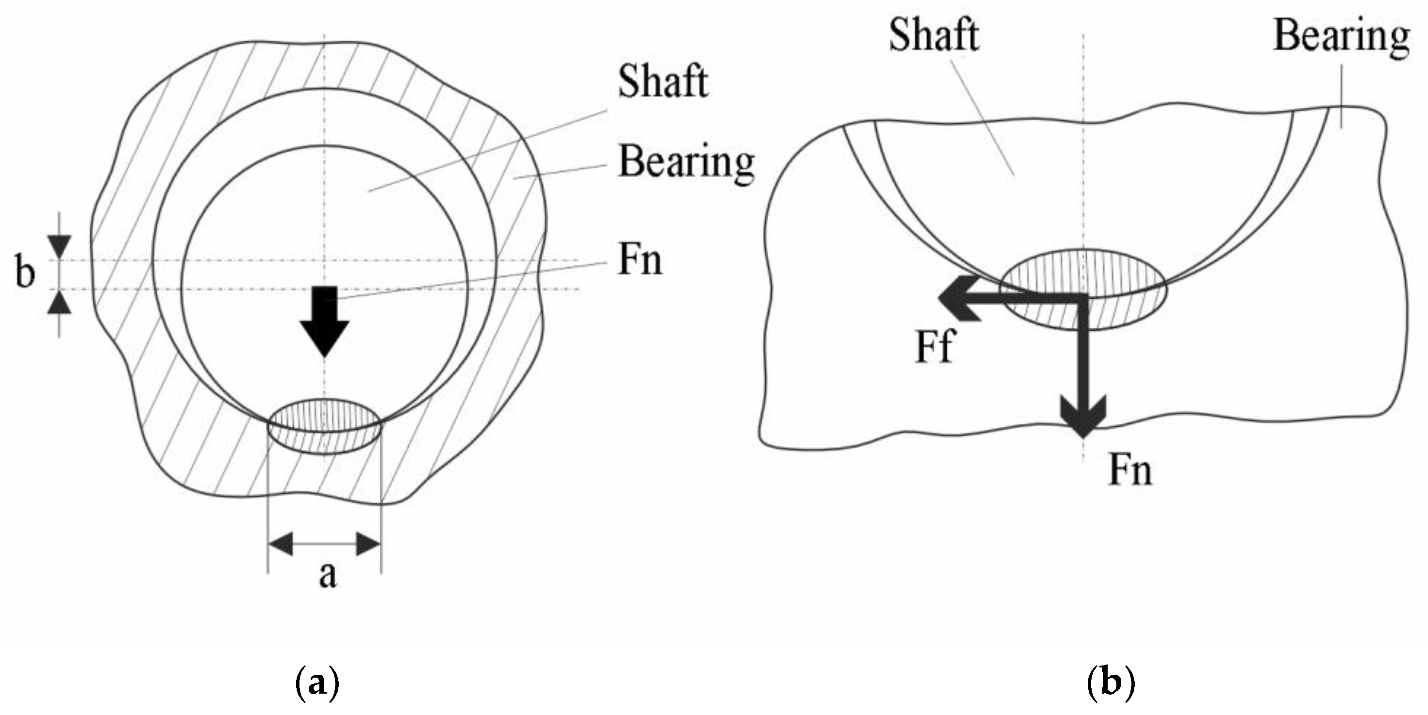
2.1. Friction Processes in Cylindrical Joints with Clearance

More common are cylindrical joints with clearance in which a rotational movement is achieved. Such joints are currently materialized by joints between shaft spindles and bearings. In principle, it is ensured that certain constructive conditions are met to prevent relative axial displacements of the shaft spindles along their axis when such displacements are not strictly necessary. It is noted that there can be direct contact between the outer cylindrical surface of the spindle and the inner one of the bearings in the case of so-called sliding bearings. On the other hand, there are bearings in which rolling elements are interposed between the shaft spindle and the cylindrical surface of the bearing body, which constitute the so-called bearing bushings. Compared to sliding bearings, ball bearings provide conditions for the development of much lower friction forces.

In most cases, the stresses to which the shaft-type parts are subjected lead to the emergence of forces that contribute to pressing the shaft spindles into the bearings intended to support the shafts. Due to these forces and, respectively, the weight of the shaft and the parts placed on the shaft, a displacement of the spindles occurs along a radial direction, which causes the axis of symmetry of the circular surface corresponding to the spindles to no longer coincide with the axis of symmetry of the circular surface in the sliding bearing and an eccentricity e to appear (Figure 1a). In the two components of the cylindrical joint, it can be observed that there are areas subjected to more intense mechanical pressing stresses. If theoretically the contact between the spindle and the bearing is made along a common generatrix of the two cylindrical surfaces of the joint, in practice, due to the elastic deformation of the superficial layers of the two components of the cylindrical joint, a contact surface with a width b is reached, which is determined by the magnitude of the mechanical stress generated by a normal force F_n resulting from the combination of the weight of the shaft and the components located on it with the forces generated by the shaft operation process.

Under the aforementioned conditions, a friction force F_f will also appear, which will oppose a possible rotation of the spindle in the bearing bore (Figure 1b), requiring an additional energy consumption to set the spindle in rotation and, respectively, to maintain the rotation when the spindle is already in rotation. It is mentioned, as such, the existence of a static friction coefficient µ_s, which manifests itself at the initiation of spindle rotation in the bearing, and, respectively, of a kinetic friction coefficient µ_k, specific to the situation in which the spindle is already rotating inside the sliding bearing.

To experimentally determine the magnitudes of the static friction coefficient µ_s and kinetic friction coefficient µ_k, respectively, it is necessary to know the magnitudes of the normal force F_n, the friction force F_f, and the specific conditions of the operation of the cylindrical joint. It is appreciated that the main factors and groups of factors that can exert influence on the magnitude of the static friction coefficients µ_s and kinetic friction µ_k are the following [1,2,3,4,5,10,11,12,13,14,15,16,17,18,19,20]:

−

The magnitude of the normal force F_n;

−

The diameter d of the circular cross-section through the spindle and the diameter D of the circular section through the bore in which the spindle is located, along with the length of the contact area between the spindle and the bearing;

−

The nature and some physical-mechanical properties of the properties of the materials from which the spindle and the sliding bearing bushing are made;

−

The heights of the asperities on the surfaces in contact with the spindle and the shaft;

−

The presence and lubricating properties of the eventual lubricant are located between the spindle and the bearing.

Especially in the case of cylindrical spindle-bearing type joints, the problem of reducing the friction that occurs when the shaft rotates inside the bearing is usually raised, researchers being, as such, interested in the intensity of the influence exerted by different factors on the friction force that occurs during the operation of a clearance cylindrical joint.

2.2. Modeling by the Finite Element Method of Specific Aspects of the Functioning of a Cylindrical Joint

Experimental tests revealed the need to highlight, if possible, stress distribution when contact is achieved only partially due to different values of clearances between the shaft and the bushing (Figure 2). It was chosen as an Ansys researcher license with its module static structural to run the finite element method (FEM).

The 3D models were designed using Siemens Solid Edge teacher edition in the form of an assembly with two distinct values for clearances between components that were constrained to share axial alignment and are tangent to one another. The models were saved as Parasolid files for easier translation to FEM, as they share the same dimensions as those experimentally tested. Ansys Space Claim was used to check for small gaps and interferences. The materials assigned to both the shaft and bushing were modeled based on structural steel for the S235 steel and generic copper retrieved from the software library. Both display isotropic behaviors, setting FEM for ideal testing conditions. As surfaces in contact have no asperities, friction phenomena were chosen to be represented by the frictional coefficient only.

The connection branch received a frictional contact between the upper surface of the shaft and the inner face of the bushing with 0.00501 for the static friction coefficient. The behavior between surfaces was set to asymmetric, and interface treatment upon geometric modification was set to adjust to touch. It also introduced a revolute joint between bodies. Mesh-wise, there were set element sizes for surfaces in contact, and a multizone method was imposed that uses a hexagonal mesh type for mapping. It produces a high-order hexagonal element type of Hex20 instead of the obsolete Hex8 with 20 nodes and Wed15 nonlinear wedge prismatic ones with 15 nodes. It gives 155,432 nodes and 34,000 elements for the model with 0.05 mm clearance and 149,629 elements and 32,606 nodes for the 0.1 mm one.

Analysis settings include three time steps with up to 150 maximum sub-steps with no weak springs.

It was aimed to highlight stress distribution for the revolving shaft as contact is achieved only on a small area given the existing clearances with and without lubrication. Results include equivalent types of stress evaluated according to von Mises criteria for all bodies as well as each one separately. A contact tool was introduced for gap and possible penetration assessment. In all cases, the gap sensor reveals a zone of the surface that is not in contact during the process, displaying values equal to clearance ones. Penetration was zero for all cases.

Values displayed are low, peaking at just 2.4275 Pa for the model with 0.05 mm in clearance and no lubrication as opposed to the model with 0.1 mm in clearance with no lubrication that registers 3.6964 Pa. A lower coefficient of friction that signals the presence of lubricant gives equivalent (von Mises) stress that peaks at 2.4289 Pa for the smaller clearance model and reaches a maximum value of 3.6969 Pa for the greater one. While lubrication lowers friction phenomena, stress distribution reveals what areas are in contact given the clearance factor. If one assesses the impact that lubrication has on surface finish, further analyses should account for the arithmetic average roughness R_a parameter. The present study aims to confirm the lubrication effect upon the friction process, and it does reveal stress distribution on contact areas, which could prove to be valuable information in designing new materials that are self-lubricants. Material design, in the field of materials science, means the activity of modifying the chemical composition or structure of a material or even generating a new material so that the material best fulfills its functional roles [21,22]. In this way, in the chemical composition of a metal alloy or a material in general, elements can be introduced that contribute to better behavior of the material in friction processes, for example.

The authors recommend that results should be treated with care since the models are ideal and do not account for eccentricities in movement that are induced by different clearances.

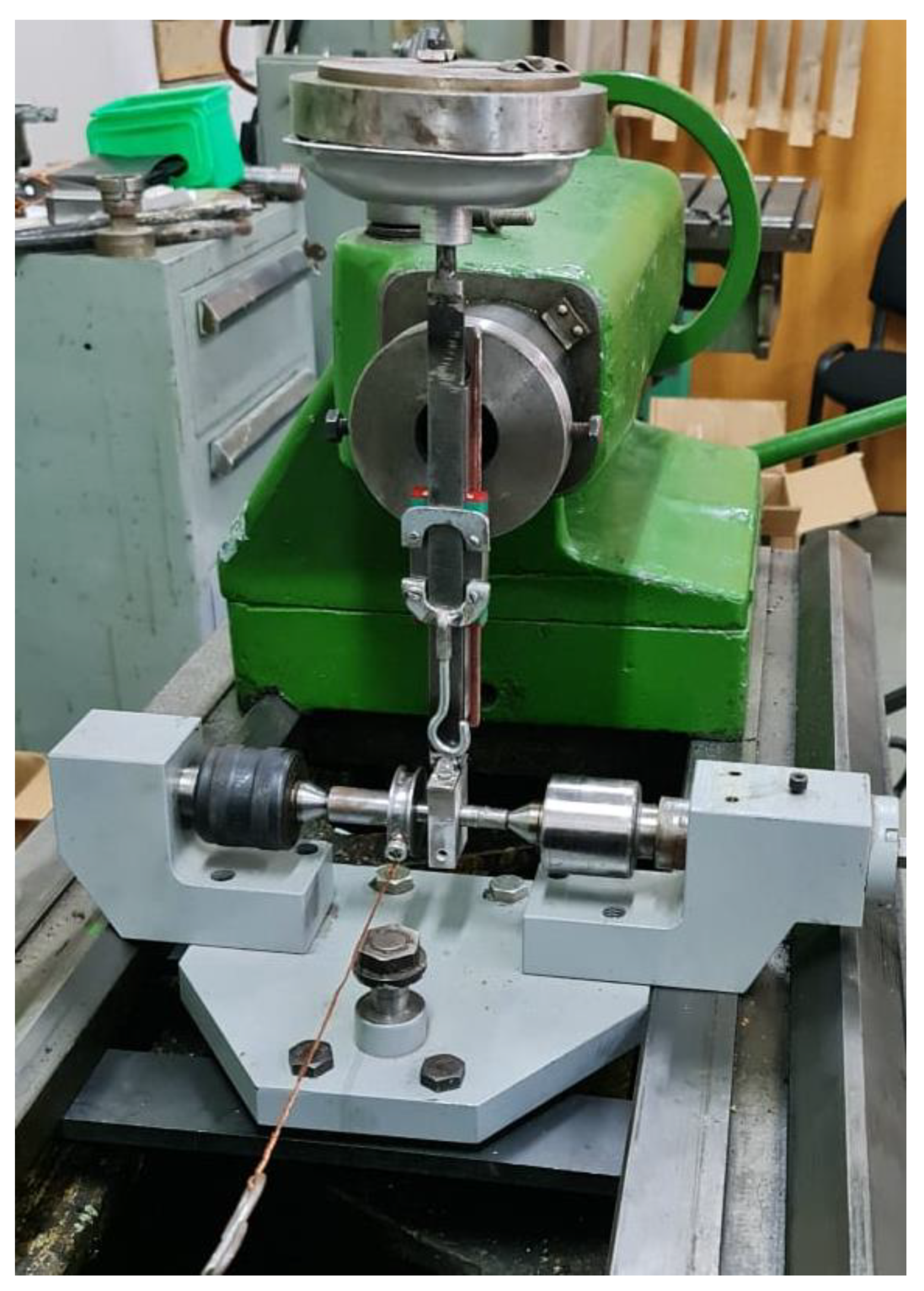
2.3. Conditions for Conducting Experimental Tests

The objective pursued by the experimental research was to determine the intensity of the influence exerted by some specific factors of the friction process in cylindrical friction joints on the magnitude of the friction coefficient under dry friction and fluid friction conditions.

To carry out the experimental tests, the use of a device adaptable to a universal lathe was considered (Figure 3 and Figure 4). The device implies the existence of a base plate, by which the device can be placed and immobilized in a certain position on the guides of the universal lathe bed. The device used aimed to simulate the operating conditions of a cylindrical joint of the spindle-bearing bushing type.

Two supports mounted on the base plate provide conditions for supporting two rotating live centers, between which a shaft equipped with a cylindrical zone corresponding to a spindle will be oriented through which, under normal conditions, it rests in a bearing. This bearing is materialized by a bushing immobilized in a parallelepiped part corresponding to the bearing body. The parallelepiped part is provided with a slot that allows the bushing to be clamped when a tightening screw is actuated. The parallelepiped part is clamped to the lower end of a vertical rod attached to a slide that can move on a guide attached to the stock quill of the universal lathe. A plate is assembled at the upper end of the vertical rod, on which weights of different sizes can be placed. These weights will allow the materialization of different pressures acting on the bearing bushing in the corresponding zone of the shaft, corresponding to different values of the normal force F_n. Another zone of the shaft was made in the form of a belt wheel on which a cable is wound, also secured to the zone in the form of a belt wheel. The other end of the cable is pulled by the cross slide of the universal lathe, to which the cable is attached using a clamp. A dynamometer was placed between the clamp and the end of the cable, with which the pulling force of the cable was measured.

When a weight is placed on the platen and the movement of the lathe carriage is initiated, pulling the cable will cause the shaft to rotate and therefore the cylindrical zone of the shaft to rotate inside the bearing bush. If the weight placed on the platen provides information about the magnitude of the normal force F_n, the force shown by the dynamometer will be proportional to the friction force F_f developed between the bearing bush and the cylindrical zone of the shaft.

Taking into account the equality of the moment generated by the force F_c of pulling the cable with the moment of the friction force F_f between the bearing bush and the cylindrical zone of radius r_s of the shaft (r_s = 5 mm; the radius corresponds to the cylindrical joint), it can be written:

$$F_c{r}_c=F_f{r}_j,$$

(1)

where r_c corresponds to the radius at which the axis of the circular cross-section through the cable on the pulley-shaped zone of the shaft is located (r_c = 13.42 mm). From relation (1), the calculation relation for the magnitude of the friction force F_f can be determined:

$$F_f={\displaystyle \frac{F_c{r}_c}{r_j}}$$

(2)

Having the magnitudes of the friction forces F_f and those of the normal force F_n, by using the known relationship, the magnitude of the friction coefficient µ can be determined:

$$\mu ={\displaystyle \frac{F_f}{F_n}}.$$

(3)

The device described above was placed and fixed on the bed guides of a universal lathe (SN250x800, TOS Trenčín, Slovacia). A shaft made of S235 steel was used, while the bearing bush was made of copper.

S235 steel is considered to be a non-alloy structural steel. This steel contains 0.15% C, 0.9% Mn, 0.03% P, and 0.04% S.

Copper was used as a material for the bearing bush test samples in the context of a larger research program, which aims to evaluate the behavior of different materials in the composition of bearings according to the specific requirements of these machine elements. In the coming period, it is intended to develop experimental research in which some of the copper alloys more often used in this regard as bearing materials are taken into account, such as, for example, some categories of bronzes. On the other hand, copper has a high thermal conductivity that could contribute to a faster evacuation of the heat generated by friction and, in this way, to a less intense wear of the bearing bushes. The very good plasticity of copper has determined the application of cold plastic deformation processing processes for the manufacture of bearing bushes [23]. There are, moreover, manufacturers of copper-bearing bushes for various destinations [24,25].

Copper is also valued as a metallic material with good antimicrobial properties, which determines its use in bearing bushings in medicine or the food industry.

The experimental tests were carried out according to the requirements of a factorial experiment of type L8, with three independent variables having values on two levels of variation.

As input factors in the investigated friction process, the normal force F_n (F_n1 = 16.16 N, F_n2 = 65.64 N) and the speed of movement of the carriage (v₁ = 200.025 mm/min, v₂ = 1800.225 mm/min) were used. A third input factor was the absence or presence of lubricant L between the outer surface of the cylindrical zone of the shaft and the inner surface of the bearing bushing.

The nominal diameter D of the cylindrical joint was 10 mm. The clearance between the two components of the joint had a value of c = 0.12 mm.

An image of the device used in the experimental research can be seen in Figure 5.

3. Results

The experimental tests aimed, first, at determining the value of the pulling force F_c from the cable for starting the rotation of the step in the form of a shaft pulley. The magnitude of this force, F_c was highlighted by the dynamometer. Subsequently, the values indicated by the dynamometer were also read during the rotation of the zone in the form of a shaft pulley. Five values of the pulling force from the cable were determined, both at the initiation of the shaft rotation and during the shaft rotation, and the values highlighted by the dynamometer were included in columns 5 and 10 of

Table 1. The 2³ full factorial experiments with the resulting static and kinetic friction coefficients.

Input Factors				Static Friction Force					Kinetic Friction Force
Run No.	Normal Force, Fn, N	Travel Speed, v, mm/min	Lubrication, L	Meas.	Avg.	St. Dev.	Ffs	μs	Meas.	Avg.	St. Dev.	Ffk	μk
1.1	16.16	200.025	−1	0.080	0.081	0.010	0.217	0.0135	0.165	0.162	0.026	0.435	0.0100
1.2				0.075					0.120
1.3				0.085					0.160
1.4				0.070					0.180
1.5				0.095					0.185
2.1	16.16	200.025	1	0.025	0.030	0.004	0.081	0.0050	0.090	0.113	0.018	0.303	0.0070
2.2				0.030					0.105
2.3				0.035					0.110
2.4				0.030					0.125
2.5				0.030					0.135
3.1	16.16	1800.225	−1	0.080	0.087	0.007	0.234	0.0054	0.250	0.287	0.022	0.770	0.0178
3.2				0.090					0.295
3.3				0.095					0.285
3.4				0.080					0.300
3.5				0.090					0.305
4.1	16.16	1800.225	1	0.020	0.031	0.010	0.083	0.0019	0.180	0.221	0.024	0.593	0.0137
4.2				0.045					0.220
4.3				0.025					0.240
4.4				0.035					0.235
4.5				0.030					0.230
5.1	65.64	200.025	−1	0.175	0.150	0.020	0.403	0.0023	0.680	0.635	0.067	1.704	0.0097
5.2				0.140					0.665
5.3				0.145					0.680
5.4				0.125					0.630
5.5				0.165					0.520
6.1	65.64	200.025	1	0.085	0.090	0.013	0.242	0.0014	0.250	0.348	0.077	0.934	0.0053
6.2				0.070					0.375
6.3				0.100					0.285
6.4				0.100					0.430
6.5				0.095					0.400
7.1	65.64	1800.225	−1	0.205	0.167	0.025	0.448	0.0025	0.715	0.667	0.103	1.790	0.0102
7.2				0.165					0.640
7.3				0.145					0.500
7.4				0.175					0.715
7.5				0.145					0.765
8.1	65.64	1800.225	1	0.145	0.141	0.011	0.378	0.0021	0.335	0.339	0.016	0.910	0.0052
8.2				0.135					0.345
8.3				0.145					0.340
8.4				0.125					0.360
8.5				0.155					0.315

. The average values of the results recorded for each situation were entered in columns 6 and 11.

In columns 7 and 12, the values of the standard deviations corresponding to each of the measurement situations can be observed.

The magnitudes of the friction forces determined using relations of the form (2) were entered in column 8 for the static friction force and in column (13) for the kinetic friction force, respectively. Finally, the magnitudes of the static friction coefficients µ_s and kinetic µ_k determined as ratios between the friction force F_f and the normal force F_n were entered in columns 9 and 14.

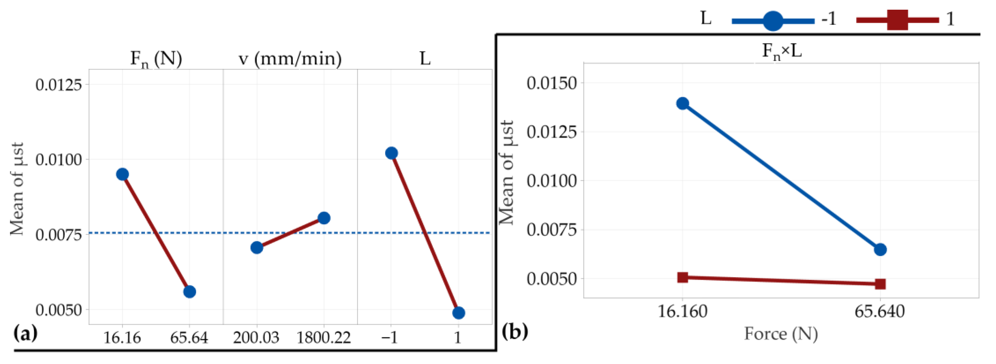
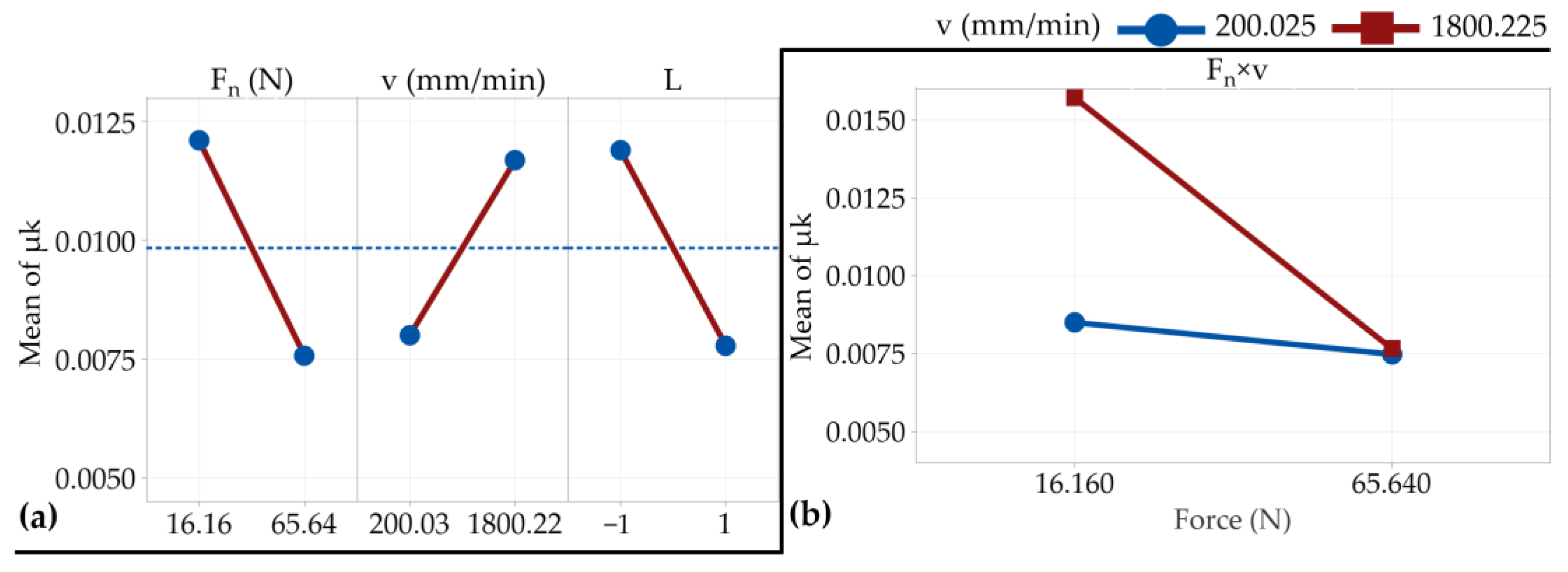
3.1. Variables Effects

The experimental data were analyzed using the statistical tool Minitab 20.1.0. All analyses were conducted at a 95% confidence level.

The independent variables’ influence on the static and kinetic friction coefficients was examined graphically using the factorial plots.

Starting with the static friction coefficient µs, it can be observed that the lubrication L is the most significant variable. As shown by the plot in Figure 6a, the lack of lubricant significantly increases the value of the friction coefficient µs. The applied force respects a similar evolution, the µ_s value decreasing when increasing the applied force normal force F_n. The travel speed v has the least significant influence and shows a slight increase of µs when switching from a low to a higher travel speed. As shown in Figure 6b, the possible interaction between the normal force Fn and lubrication L was identified. However, for the studied force levels, the interaction cannot be considered highly significant. Using other levels of the normal force Fn could help determine if the interaction significantly explains the evolution of the friction coefficient µs.

Addressing the problem of the kinetic friction coefficient µ_k, the factorial plots shown in Figure 7 highlight that the normal force F_n is the most significant variable, which is followed by the lubrication L and the travel speed v. All three variables correspond to the same path of evolution discussed for the µ_s. However, for µ_k, the variables have even more influence over the value of the kinetic friction coefficient µ_k. Regarding the variable’s interactions, it was observed that the combined effect of force F_n and travel speed v significantly influenced the value of the kinetic friction coefficient µ_k. The interaction plot illustrated in Figure 7b indicates that a higher force F_n, regardless of the travel speed v, is preferable for obtaining lower values of the kinetic friction coefficient µ_k.

3.2. Regression Analysis

The regression analyses were conducted for a risk factor α = 0.05. As the analyzed variables have different natures (i.e., normal force F_n, travel speed v), the continuous variables were standardized by subtracting the mean and dividing it by the standard deviation. This way the analyzed continuous variables are comparable in effect and magnitude. The Pareto charts of the standardized effects displayed in Figure 8a (for µ_s) and Figure 8a (for µ_k) complete the image of the variable influence and interaction significance.

The results of using the analysis of variance (ANOVA) of the friction coefficient µ_s, whose results were included in

Table 2. Analysis of variance applied in the case of the static friction coefficient µ_s.

Source	DF	Seq SS	Contrib.	Adj SS	Adj MS	F-Value	p-Value	VIF
Regression	4	0.000573	93.40%	0.000573	0.000143	123.86	0.000
Fn	1	0.000153	24.90%	0.000279	0.000279	241.44	0.000	2.00
v	1	0.000010	1.59%	0.000010	0.000010	8.41	0.006	1.00
L	1	0.000283	46.20%	0.000283	0.000283	245.08	0.000	1.00
Fn L	1	0.000127	20.72%	0.000127	0.000127	109.89	0.000	2.00
Error	35	0.000040	6.60%	0.000040	0.000001
Lack-of-Fit	3	0.000005	0.80%	0.000005	0.000002	1.48	0.240
Pure Error	32	0.000036	5.80%	0.000036	0.000001
Total	39	0.000613	100.00%

Note. The meanings of the symbols are as follows: DF degrees of freedom; Seq SS–sequential sum of squares; Contrib. –the percentage that each factor contributes to the total sequential sums of squares; Adj SS measures of variation for different factors of the model; F-Value—the test statistic considered used to appreciate whether the model could be associated with the response: p-Value—probability used to measure the evidence against the null hypothesis; VIF—variance inflation factor, which indicated the increase in a regression coefficient as a result of collinearity.

, were considered in generating Equation (4) in statistical terms. According to the F-Value and their p-Values under 0.005, all models’ terms contribute to the evaluation of the estimation model. However, based on the variance inflation factor (VIF) value of 2.00, the normal force F_n variable and the interaction force F_n ∙lubrication L have a moderate degree of multicollinearity. In other words, there is a moderate indication that there is a correlation between the aforementioned factors. This means that modifying a variable value is influencing the variation of the other one.

The empirical mathematical model determined in the case of the static coefficient µ_s is the following:

$${\mu }_s=0.010168-0.000079F_N+0.000001v-0.005607L+0.000072 F_{n}L.$$

(4)

By looking at the information available in

Table 3. Evaluation of the static friction coefficient µ_s mathematical model.

S	R2	R2(adj)	PRESS	R2(pred)	AICc	BIC
0.0010750	93.40%	92.65%	0.0000528	91.38%	−424.11	−416.52

, it can be seen that there is a good estimation capacity of the measurement variability of 93.40% (coefficient of determination R²), in which the Equation (4) terms contribute to 92.65% (R²adj) of the estimation capacity. This leads to an overall prediction capacity of 91.38% (R²pred) with a standard deviation S of 0.001075 and a low value of predicted residual error sum of squares (PRESS). Furthermore, the good fit of the resulting model is highlighted by the residual plot shown in Figure 9b. To avoid possible multicollinearities, the interaction term was removed to ensure the regression model’s estimation and prediction stability. Even more, AIC (Akaike’s information criterion) and BIC (Bayesian information criterion) are both very low, indicating a well-balanced model in terms of fit and complexity.

Going further, the results of applying the analysis of the variance (ANOVA) in the case of the kinetic friction coefficient µ_k are detailed in

Table 4. Analysis of variance applied in the case of the kinetic friction coefficient µ_k.

Source	DF	Seq SS	Contrib.	Adj SS	Adj MS	F-Value	p-Value	VIF
Regression	4	0.000636	91.90%	0.000636	0.000159	99.31	0.000
Fn	1	0.000206	29.77%	0.000206	0.000206	128.65	0.000	1.00
v	1	0.000136	19.71%	0.000136	0.000136	85.17	0.000	1.00
L	1	0.000170	24.55%	0.000170	0.000170	106.13	0.000	1.00
Fn × v	1	0.000124	17.88%	0.000124	0.000124	77.28	0.000	1.00
Error	35	0.000056	8.10%	0.000056	0.000002
Lack-of-Fit	3	0.000005	0.73%	0.000005	0.000002	1.06	0.382
Pure Error	32	0.000051	7.37%	0.000051	0.000002
Total	39	0.000692	100.00%

. These results summarize the significance of the variables considered in Equation (5). All models’ terms show significant importance to the data variability estimation as they have high F-Values and 0.000 p-Values. The resulting empirical model includes all three independent variables and the normal force Fn- lubrication L interaction.

As a result of the mathematical processing of the experimental results using the Minitab 20.3 software, the following empirical mathematical model was determined:

$${\mu }_k=0.007654-0.000003F_n+0.000006v-0.002061L-0.000000F_{n}v$$

(5)

The data available in

Table 5. Mathematical model summary in the case of the kinetic friction coefficient µ_k.

S	R2	R2(adj)	PRESS	R2(pred)	AIC	BIC
0.0012651	91.90%	90.98%	0.0000732	89.42%	−411.09	−403.50

summarize the µ_k regression model quality. According to the value of the coefficient of determination R², the empirical model explains 91.90% of the measurements’ variability, as the selected terms explain 90.98% (R²adj) of the Table 1 data. Overall, the model has a prediction capacity of 89.42% (R²pred) with a standard deviation S of 0.0012651 together with a low value of PRESS value. As highlighted by the normal probability plot from Figure 9b, the model shows low residuals. Nevertheless, according to the low values of AIC and BIC criteria, the regression model corresponding to the kinetic friction coefficient µ_k is a good fitting model.

The coefficient of determination R², both for the static friction coefficient (Table 3) and for the kinetic friction coefficient (Table 5), has values higher than 90%, which highlights the fact that the proposed empirical mathematical models are in good correspondence with the experimental results obtained.

By dividing the resulting friction coefficients based on the lubrication usage through the normal probability plots illustrated (Figure 10), it can be observed that a part of the recorded data are distributed across a wider range of variation. During the experimental tests, the stick-slip phenomenon was observed when driving the lathe carriage. This could explain why a part of the recorder data are unevenly clustered.

By taking into account the empirical mathematical models constituted by Equations (4) and (5), the graphical representations in Figure 11, Figure 12 and Figure 13 were developed.

The analysis of the mathematical models corresponding to Equations (4) and (5) and the graphical representations developed based on them allowed the formulation of the following observations.

It is thus found, first of all, that, among the input factors taken into account, the strongest influence on both the magnitude of the static friction coefficient µ_s and the magnitude of the kinetic friction µ_k coefficient is exerted by the presence or absence of the lubricant L, since in the first-degree polynomial Equations (4) and (5), the coefficient allocated to highlighting the influence of the lubricant L has an absolute value greater than the absolute values of the coefficients corresponding to the other two input factors in the analyzed process. It is found, at the same time, that the coefficient assigned to the factor L has a negative value, which means that the presence of the lubricant in the cylindrical joint causes a decrease in the magnitude of the static friction coefficient µ_s. Such an observation is consistent with the initial hypothesis according to which the presence of the lubricant leads to a reduction in the magnitude of the friction force F_f and therefore of the values of the static friction coefficients and, respectively, of the kinetic friction coefficients.

In the case of the static friction coefficient µ_s, from the point of view of the influence exerted, the magnitude of the normal force F_n is in second place, the coefficient assigned to this factor having values between the values of the coefficients assigned to the factors L and v. Since it is talking about the static friction force F_fs, which occurs when the shaft is set in motion inside the bore, the greater influence of the magnitude of the normal force F_n is justified, compared to the influence of the speed v. It is also noted that a certain influence is exerted by the interaction between the normal force F_n and the presence of the lubricant L, the increase in the value of this interaction leading to an increase in the value of the static friction coefficient.

According to the graphic representation in Figure 11, it is found that with the increase in the magnitude of the normal force F_n, there is a slight decrease in the values of the static and kinetic friction coefficients. This result could be related to the so-called Rehbinder effect. In principle, the Rehbinder effect refers to the decrease in the hardness and ductility of some metallic materials, including those due to the presence of a surfactant film. The use of grease in the cylindrical joint could thus lead to a reduction in the magnitude of the friction force, as is the case with the use of other categories of lubricants [13,14].

It is appreciated that the development of friction and wear processes in cylindrical joints has been an objective of theoretical and experimental research activities [1,2,3,4,5,9,11,16,17,18,19,20]; such research provides valid explanations, including for the processes investigated experimentally and presented in this paper.

In the case of the coefficient of kinetic friction µk, the second most important factor in terms of the influence exerted on the magnitude of the coefficient µk is the travel speed v, the increase in speed v leading to an increase in the value of the coefficient of kinetic friction µk, since the value of the coefficient corresponding to the speed v is positive. It was also expected that an increase in the peripheral speed v would result in an increase in the magnitude of the friction force Ff and therefore in the magnitude of the coefficient of kinetic friction µk.

4. Conclusions

Understanding the importance of the coefficient of friction in cylindrical clearance joints is essential for estimating the energy required to overcome the friction forces in different systems. It is considered that the main key points of the research carried out are the following:

• The finite element modeling of the friction processes in cylindrical clearance joints facilitated the evaluation of the equivalent stresses for different dimensions of the clearance between the shaft and the bore.
• An adaptable device was designed and adapted on a universal lathe to facilitate the measurement of the magnitudes of the friction force under controlled conditions, allowing the variation of the normal force, the relative velocity, and the lubrication.
• Experimental tests were carried out to evaluate the influence of key factors, such as the magnitude of the normal force, the relative velocity between the shaft and the bore, and the presence or absence of a lubricant, on the magnitude of the static and kinetic friction coefficients. The experiments were conducted using a full factorial experiment with three independent variables, each tested at two levels of variation.
• The experimental results were processed mathematically using specialized software. Empirical mathematical models of the first-degree polynomial type were determined. These empirical mathematical models quantify the influence of each input factor on the static and kinetic friction coefficients.
• Among the factors studied, the presence or absence of lubricant was identified as having the most significant impact on the magnitudes of both friction coefficients.
• Future research aims to investigate various other material pairs for cylindrical clearance joint components and to incorporate additional input factors into the experiments.

References

1. Tian, Q.; Liu, C.; Machado, M.; Flores, P. A new model for dry and lubricated cylindrical joints with clearance in spatial flexible multibody systems. Nonlinear Dyn. 2011, 64, 25–47. [Google Scholar] [CrossRef]
2. Theory for Friction in Joints. Available online: https://doc.comsol.com/5.4/doc/com.comsol.help.mbd/mbd_ug_theory.4.20.html (accessed on 11 November 2024).
3. Todi-Eftimie, A.; Bobancu, S.; Gavrila, C.; Eftimie, L. Static friction coefficient into cylindrical joints assemblies. Tribol. Ind. 2015, 37, 421–426. Available online: https://www.tribology.rs/journals/2015/2015-4/4.pdf (accessed on 14 September 2024).
4. Liu, C.; Zhang, K.; Yang, L. Compliance contact model of cylindrical joints with clearances. Acta Mech. Sin. 2005, 21, 451–458. Available online: https://link.springer.com/article/10.1007/s10409-005-0061-7 (accessed on 17 September 2024). [CrossRef]
5. Stamenkovic, D.; Milosevic, M.; Mijajlovic, M.; Banic, M. Estimation of the static friction coefficient for press fit joints. J. Balk. Tribol. Asso. 2011, 17, 341–355. Available online: https://www.researchgate.net/publication/241688933_Estimation_of_the_static_friction_coefficient_for_press_fit_joints (accessed on 17 September 2024).
6. Tadić, B.; Kočović, V.; Matejić, M.; Brzaković, L.; Mijatović, M.; Vukelić, Đ. Static coefficient of rolling friction at high contact temperatures and various contact pressure. Tribol. Ind. 2016, 38, 83–89. Available online: https://www.researchgate.net/publication/301043681_Static_Coefficient_of_Rolling_Friction_at_High_Contact_Temperatures_and_Various_Contact_Pressure (accessed on 19 September 2024).
7. Rung, S.; Bokan, K.; Kleinwort, F.; Schwarz, S.; Simon, P.; Klein-Wiele, J.-H.; Esen, C.; Hellmann, R. Possibilities of dry and lubricated friction modification enabled by different ultrashort laser-based surface structuring methods. Lubricants 2019, 7, 43. [Google Scholar] [CrossRef]
8. Tauviqirrahman, M.; Jamari, J.; Wicaksono, A.A.; Muchammad, M.; Susilowati, S.; Ngatilah, Y.; Pujiastuti, C. CFD analysis of journal bearing with a heterogeneous rough/smooth surface. Lubricants 2021, 9, 88. [Google Scholar] [CrossRef]
9. Millan, P.; Pagaimo, J.; Magalhães, H.; Ambrósio, J. Clearance joints and friction models for the modelling of friction damped railway freight vehicles. Multibody Syst. Dyn. 2023, 58, 21–45. [Google Scholar] [CrossRef]
10. Aleem, M.; Saad, A.A.; Sohail, A.; Siraj, S.M.; Reddy, M.R. Design and analysis of drum brakes. Int. J. Adv. Innov. Res. 2018, 10, 0348–0354. Available online: https://www.ijatir.org/uploads/541362IJATIR16691-64.pdf (accessed on 21 September 2024).
11. Dinescu, I.; Bardocz, G. Experimental research on the variation of coefficient of friction in sliding bearings. Științe Teh. Și Mat. Apl. 2006, 7–14. Available online: https://www.afahc.ro/ro/revista/Nr_1_2006/1.pdf (accessed on 22 September 2024). (In Romanian).
12. Leonov, O.A.; Shkaruba, N.Z.; Vergazova, Y.G. Calculation of the maximum functional clearance of a cylindrical joint between a steel shaft and a cast iron sprocke. CIS Iron Steel Rev. 2024, 27, 108–112. Available online: https://rudmet.net/media/articles/Article_CIS_2024_27_pp.108-112.pdf (accessed on 22 September 2024). [CrossRef]
13. Qiu, T.; Yan, L.; Wang, F.; Xie, H.; Shui, Y.; Zhang, T.; Jiang, F. Research advances of Rehbinder effect in material removal process. China Surf. Eng. 2024, 37, 59–74. [Google Scholar] [CrossRef]
14. Chaudhari, A.; Soh, Z.Y.; Wang, H.; Kumar, A. Senthil. Rehbinder effect in ultraprecision machining of ductile materials. Int. J. Mach. Tools Manuf. 2018, 133, 47–60. [Google Scholar] [CrossRef]
15. Liu, X.; Wang, Y.; Qin, L.; Guo, Z.; Lu, Z.; Zhao, X.; Dong, H.; Xiao, Q. Friction and wear properties of a novel interface of ordered microporous Ni-based coating combined with MoS2 under complex working conditions. Tribol. Int. 2023, 189, 108970. [Google Scholar] [CrossRef]
16. Liu, X.; Guo, Z.; Lu, Z.; Qin, L. Tribological behavior of the wear-resistant and self-lubrication integrated interface structure with ordered micro-pits. Surf. Coat. Technol. 2023, 454, 129159. [Google Scholar] [CrossRef]
17. Kamga, L.S.; Meffert, D.; Magyar, B.; Oehler, M.; Sauer, B. Simulative investigation of the influence of surface texturing on the elastohydrodynamic lubrication in chain joints. Tribol. Int. 2022, 171, 107564. [Google Scholar] [CrossRef]
18. Pereira, C.; Ambrosio, J.; Ramalho, A. Contact mechanics in cylindrical clearance revolute joints. Appl. Mech. Mater. 2013, 365–366, 412–415. [Google Scholar] [CrossRef]
19. Pereira, C.; Ramalho, A.; Ambrosio, J. Applicability domain of internal cylindrical contact force models. Mech. Mach. Theory 2014, 78, 141–157. [Google Scholar] [CrossRef]
20. Liu, C.-S.; Zhang, K.; Yang, R. The FEM analysis and approximate model for cylindrical joints with clearances. Mech. Mach. Theory 2007, 42, 183–197. [Google Scholar] [CrossRef]
21. Lookman, T.; Balachandran, P.V.; Xue, D.; Hogden, J.; Theiler, J. Statistical inference and adaptive design for materials discovery. Curr. Opin. Solid State Mater. Sci. 2017, 21, 121–128. [Google Scholar] [CrossRef]
22. Sutton, A.P. Materials by design. In Concepts of Materials Science, Online ed.; Oxford Academic: Oxford, UK, 2021. [Google Scholar] [CrossRef]
23. Hong, X.; Xu, H.; Xu, Y.; Huang, T.; Guo, Y.; Zhang, J.; Peng, Y. Study on spinning process parameters of the copper bushing by tribological properties and physical testing. In Proceedings of the 2021 2nd International Conference on Applied Physics and Computing (ICAPC 2021), Ottawa, Canada, 8–10 September 2021; Volume 2083, p. 022084. [Google Scholar] [CrossRef]
24. Copper Bushing for Crawler Crane Track Roller. Available online: https://www.tradekorea.com/product/detail/P757318/Copper-bushing-for-crawler-crane-track-roller-.html (accessed on 20 January 2025).
25. Automobile Copper Bushing. Available online: https://www.indiamart.com/proddetail/automobile-copper-bushing-1894301530.html?srsltid=AfmBOopsQbMRPvZF5_GzVWmXrQ2MW_uvva33BFLVSAiGqaazcetjqzOU (accessed on 20 January 2025).
Figure 1. The occurrence of an eccentricity e in the case of a cylindrical joint with clearance (a) and, respectively, of a friction force Ff opposing the rotation of the shaft spindle (b).
Lubricants 13 00066 g001
Figure 2. Plots of gap probe and equivalent (von Mises) stress distribution: (a) gap for model with 0.05 mm clearance; (b) equivalent stress for model with 0.05 mm clearance and no lubrication; (c) equivalent stress for model with 0.05 mm clearance with lubrication; (d) gap for model with 0.1 mm clearance; (e) equivalent stress for model with 0.1 mm clearance and no lubrication; (f) equivalent stress for model with 0.1 mm clearance with lubrication.
Lubricants 13 00066 g002
Figure 3. Device adaptable to a universal lathe and intended for measuring the friction force in the case of a cylindrical joint: (a) side view; (b) top view.
Lubricants 13 00066 g003
Figure 4. Attaching the normal force generation subsystem to the front surface of the quill in the tailstock of the universal lathe.
Lubricants 13 00066 g004
Figure 5. Image of the experimental stand used for testing. For the experimental tests of lubricated friction, a grease of the MOL Liton LTA 3EP type (made by MOL Lubricants, Budapest, Hungary) was used. According to the manufacturer’s instructions, this grease is a multipurpose lubricating grease containing a highly refined mineral oil and lithium 12-hydroxystearate thickener. During the manufacturing process, additives capable of reducing wear, inhibiting oxidation and corrosion, as well as extreme pressure additives that contribute to improving the performance of the grease, were introduced into the lubricant.
Lubricants 13 00066 g005
Figure 6. Static friction coefficient µs: (a) main effect plots; (b) interaction plot.
Lubricants 13 00066 g006
Figure 7. Kinetic friction coefficient µk: (a) main effect plots; (b) interaction plot.
Lubricants 13 00066 g007
Figure 8. Static friction coefficient µs; (a) Pareto chart of the standardized effects; (b) normal probability plot of residuals.
Lubricants 13 00066 g008
Figure 9. Kinetic friction coefficient µk: (a) Pareto chart of the standardized effects; (b) normal probability plot of residuals.
Lubricants 13 00066 g009
Figure 10. Normal probability plot of the response variables for (a) static friction coefficient µs; (b) kinetic friction coefficient µk.
Lubricants 13 00066 g010
Figure 11. The influence of the normal force Fn over the static friction coefficient μs and the kinetic friction coefficient µk values (speed v = 1000 mm/min, L = +1, lubricant grease type: MOL Liton LTA3EP).
Lubricants 13 00066 g011
Figure 12. The influence of the speed v over the static friction coefficient μs and the kinetic friction coefficient µk values (normal force Fn = 40 N, L = +1, lubricant: grease type: MOL Liton LTA3EP).
Lubricants 13 00066 g012
Figure 13. The influence of the presence of lubricant on the values of the static friction coefficient µs and the kinetic friction coefficient µk for different values of the normal force Fn (speed v = 1000 mm/min, L = −1, represented by black lines, and L = + 1, represented by blue lines, lubricant: grease type: MOL Liton LTA3EP).
Lubricants 13 00066 g013