A Fusion Estimation Method for Tire-Road Friction Coefficient Based on Weather and Road Images

Abstract

The tire-road friction coefficient (TRFC) is a critical parameter that significantly influences vehicle safety, handling stability, and driving comfort. Existing estimation methods based on vehicle dynamics suffer from a substantial decline in accuracy under conditions with insufficient excitation, while vision-based approaches are often limited by the generalization ability of their datasets, making them less effective in complex and variable real-driving environments. To address these challenges, this paper proposes a novel, low-cost fusion method for TRFC estimation that integrates weather conditions and road image data. The proposed approach begins by employing semantic segmentation to partition the input images into distinct regions—sky and road. The segmented images will be fed into the road recognition network and the weather recognition network for road type and weather classification. Furthermore, a fusion decision tree incorporating an uncertainty modeling mechanism is introduced to dynamically integrate these multi-source features, thereby enhancing the robustness of the estimation. Experimental results demonstrate that the proposed method maintains stable and reliable estimation performance even on unseen road surfaces, outperforming single-modality methods significantly. This indicates its high practical value and promising potential for broad application.

1. Introduction

Road traffic safety remains a critical global concern. With the rapid advancement of the automotive industry and electronic control technologies, Advanced Driving Assistance Systems (ADAS) and Autonomous Driving (AD) technologies are increasingly becoming standard features in modern vehicles. The core mission of these systems is to enhance driving safety, optimize ride comfort, and reduce driver workload [1]. However, the fundamental prerequisite for both ADAS and AD algorithms to achieve safe and efficient vehicle control lies in the accurate perception of the vehicle and its external environment [2,3]. Among various environmental factors, the tire-road friction coefficient (TRFC)—a key physical parameter characterizing the limits of longitudinal and lateral force transmission between the tire and the road surface—directly influences braking distance, steering limits, and driving efficiency [4]. It is undoubtedly one of the most critical variables in vehicle control systems.

Moreover, accurate estimation of TRFC is also essential for improving driving comfort and optimizing vehicle energy economy. Smooth acceleration, deceleration, and cornering require the control system to operate delicately within a range that approaches, but never exceeds, the physical limits of traction. Furthermore, for AD systems aiming to make fully independent decisions, precise road friction information is a prerequisite for global path planning and local trajectory generation. Examples include predicting a safe speed ahead of a curve or adopting more conservative driving strategies in adverse weather conditions.

Therefore, research into highly reliable and low-cost TRFC estimation methods holds significant theoretical value and engineering importance for overcoming current performance limitations of ADAS, ensuring driving safety, and enhancing overall travel quality. This paper focuses on an in-depth investigation of a fusion-based TRFC estimation technique that utilizes weather and road image information, aiming to provide key technical support for the development of safer and more intelligent next-generation vehicle control systems.

2. Related Work

For mass-produced vehicles equipped with conventional sensors, the TRFC is a parameter that cannot be measured directly. Numerous scholars have developed various methods to estimate TRFC, which can be broadly categorized into two types: cause-based methods and effect-based methods. The former typically requires additional sensors to measure and analyze factors influencing friction variation—such as road texture and tire contact characteristics—to estimate TRFC. The latter focuses on analyzing the dynamic response of the vehicle during driving to infer the friction coefficient based on vehicle dynamics [5].

TRFC is complexly influenced by multiple factors including road material, surface conditions (e.g., dry or wet), tire properties, and temperature. Quan et al. deployed PVDF piezoelectric films in the tire inner liner to develop an intelligent tire model. Using finite element analysis and neural networks to estimate tire forces, they achieved high-precision TRFC estimation (with an error of 5.14%) via a brush model optimized with a genetic algorithm [6]. In addition to piezoelectric sensors, tri-axial accelerometers are also commonly used in intelligent tires. Zou et al. transformed acceleration signals into a rotating coordinate system to extract contact patch length and lateral tire deformation directly from longitudinal and lateral acceleration features. They estimated the friction coefficient using a brush model fitted via least squares [7]. Differing from vehicle-state-focused methods, Yu et al. systematically investigated the coupling effects of multiple factors such as road texture, tire pressure, and speed, and applied a BP neural network to predict macroscopic road friction coefficients [8]. Han et al. focused on road roughness and texture, proposing a TRFC estimation method that considers effective contact characteristics between the tire and three-dimensional road surfaces. By integrating an effective contact area ratio into the LuGre tire model and optimizing vertical force transmission with a multi-point contact method, they achieved estimation using normalization and an unscented Kalman filter [9].

Ye et al. introduced an adaptive tire stiffness-based TRFC estimation method. By analyzing the relationship between tire–road contact patch length and vertical load, they established an adaptive theoretical model for tire stiffness and incorporated it as a state variable into an improved fast-converging square-root cubature Kalman filter. This significantly enhanced estimation accuracy and convergence speed under various driving conditions, including extreme scenarios such as tire damage [10]. Tao et al. proposed a two-stage TRFC estimation scheme based on two robust proportional multiple integral observers and a multilayer perceptron. By introducing a threshold screening mechanism to filter out invalid data frames, the accuracy and generalization capability of the MLP estimator were substantially improved [11]. Zhang et al. developed a TRFC estimation framework based on a novel tire model and an improved square-root cubature Kalman filter (ISCKF). The novel tire model adaptively computes stiffness and effective friction coefficients to enhance force calculation accuracy, while the ISCKF adaptively updates measurement noise covariance based on the maximum correntropy criterion. This approach demonstrates strong robustness against abnormal noise interference and good adaptability to uncertainties in road friction distribution [12].

However, most effect-based methods rely heavily on model accuracy and external excitation; their performance degrades significantly under low-excitation conditions. To overcome these limitations, many researchers have combined the strengths of various approaches to develop optimized fusion estimation methods. Wang et al. proposed a TRFC estimation framework that integrates event-triggered cubature Kalman filtering (ETCKF) with an extended Kalman neural network (EKFNet). The ETCKF handles sensor data loss, while the EKFNet uses a neural network to predict Kalman gains and optimize estimation performance [13]. Zhao et al. introduced an adaptive TRFC estimation framework that fuses visual and vehicle dynamic information. Multi-temporal image fusion technology was employed to enhance road condition recognition, combined with a residual adaptive unscented Kalman filter (UKF) to improve estimation accuracy and robustness [14].

In terms of environmental perception, weather is a critical factor affecting TRFC and can be used to assist in its estimation. With the rapid development of deep learning, convolutional neural networks have demonstrated remarkable performance in various computer vision tasks, leading to their widespread use in weather recognition. Xia et al. developed a simplified model termed ResNet15 based on ResNet50. Using convolutional layers of ResNet15 to extract weather features, the model incorporates four residual modules to facilitate feature propagation via shortcuts, followed by a fully connected layer and a Softmax classifier for weather image classification [15]. Xiao et al. proposed MeteCNN, a novel CNN architecture based on VGG16, which embeds squeeze-and-excitation attention modules and introduces dilated convolutions (dilation rate = 2) in the initial and final convolutional layers. This model achieved a classification accuracy of 92.68% on a self-built dataset, outperforming mainstream models such as VGG, ResNet, and EfficientNet [16]. However, these methods rely solely on CNN features for weather classification, neglecting weather-sensitive cues such as illumination changes and contrast variations, which limits their accuracy. Li et al. proposed a multi-feature weighted fusion method that extracts handcrafted weather-related features (e.g., haze, contrast, brightness) and fuses them with CNN features into a high-dimensional vector for weather image classification. This approach improved weather recognition accuracy compared to using CNN features alone [17]. Nevertheless, manually extracting various weather features is cumbersome and requires extensive parameter tuning, resulting in poor robustness.

Although many researchers have applied neural networks to recognize road conditions, limited dataset diversity often restricts the generalization capability of these models, leading to unreliable performance in complex and varying driving environments. Studies have shown that directly using neural network outputs can cause oscillatory predictions, which is detrimental to TRFC estimation [18,19,20,21]. Guo et al. proposed a vision-vehicle dynamics fusion framework for estimating peak TRFC. A lightweight CNN identifies road type to determine a friction coefficient range, while a UKF estimates the friction coefficient based on vehicle dynamic states. After spatiotemporal synchronization, a confidence-based fusion strategy refines the final result [22]. Although this confidence-based fusion reduces the impact of misclassified road images, the vision-based module fails to provide a stable and correct friction coefficient range when the vehicle encounters unseen road types not included in the training dataset.

To address these challenges, this paper innovatively proposes a fusion estimation method for TRFC that utilizes both weather and road image information, without requiring additional sensors—only a single onboard camera. The contributions of this work are as follows:

(1)

We incorporate the Efficient Channel Attention (ECA) mechanism into MobileNetV4-ConvSmall, achieving an accuracy of 95.63% in recognizing 15 different road types while maintaining a lightweight model architecture.

(2)

We develop a lightweight three-branch convolutional neural network that simultaneously captures sky, road, and global image features for effective weather recognition.

(3)

We propose a novel fusion strategy that accounts for uncertainties in both road and weather recognition. This approach enables reliable estimation even when the road type is unseen or recognition results are unreliable, significantly enhancing system robustness.

3. Proposed Method

3.1. Overall Architecture

The proposed architecture is illustrated in Figure 1. The image captured by the onboard camera is first fed into a semantic segmentation network, which partitions it into two regions: road, and sky. The road image is then input to a road recognition network, while the road, sky, and the original image are passed to a three-branch convolutional neural network for weather recognition. These networks output the road type, weather type, and their corresponding classification probability distributions. A fusion decision tree selects an appropriate strategy based on the road and weather information, which is then provided to the TRFC filter. The TRFC filter performs joint Gaussian distribution modeling, friction coefficient correction, uncertainty modeling, and filtering estimation to produce the final TRFC estimate.

3.2. Semantic Segmentation

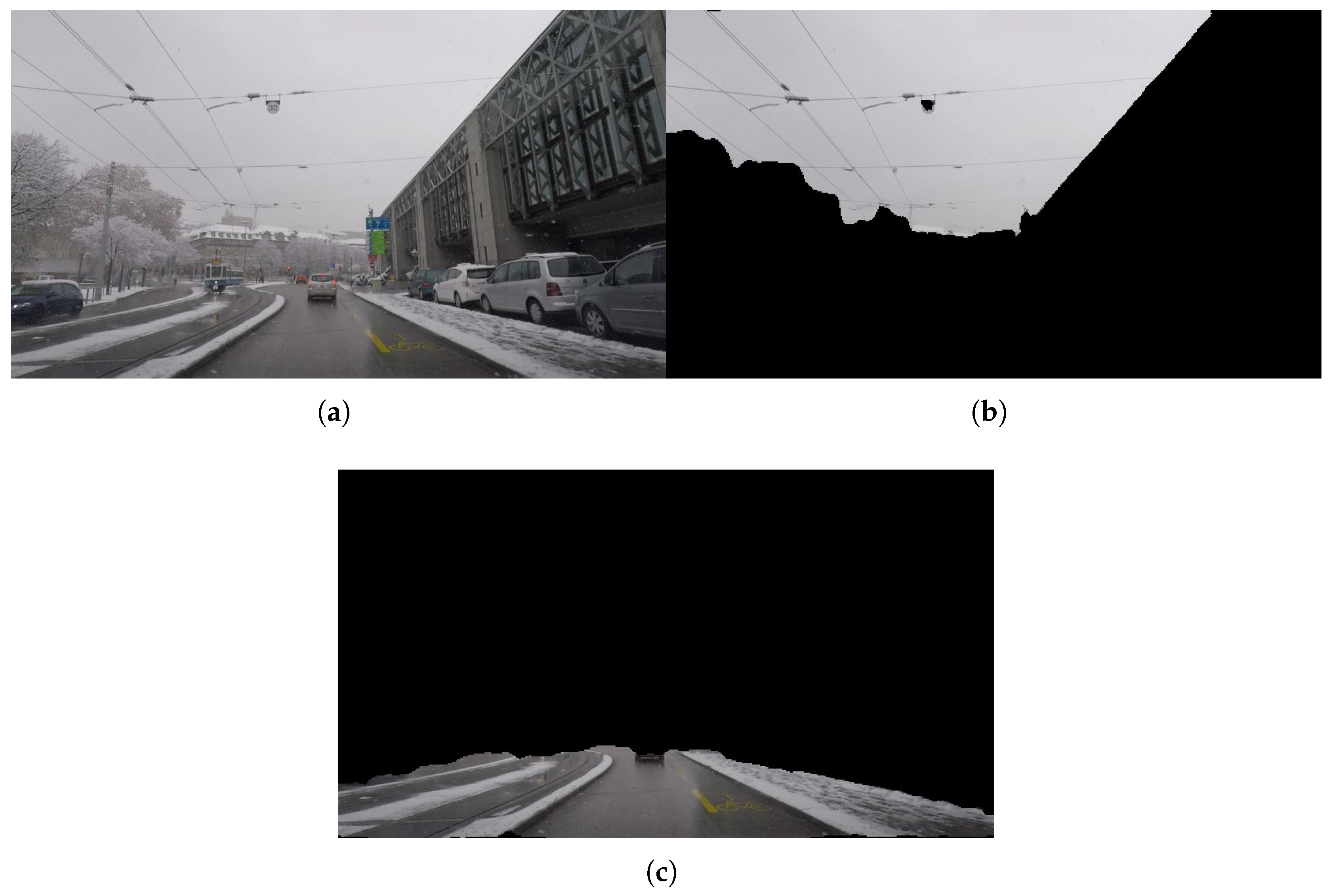
To facilitate the recognition of sky and road regions, the original image must be segmented. As shown in the Figure 2, the segmented regions consist of the road and sky. Semantic segmentation requires a road dataset with pixel-level annotations for precise partitioning. The segmentation network was trained on the Cityscapes dataset [23], which contains 5000 finely annotated urban scene images. We retained only two semantic categories—road and sky—for this task. The dataset was split into 60% for training, 20% for validation, and 20% for testing.

We adopt DeepLabv3+ [24] with MobileNetV2 as the backbone for semantic segmentation. The model consists of an encoder and a decoder. The encoder is based on DeepLabV3 and employs an Atrous Spatial Pyramid Pooling (ASPP) module, which uses multi-scale dilated convolutions to capture rich contextual information. The decoder gradually upsamples the feature maps and incorporates shallow features from the backbone through skip connections to recover detailed information and improve boundary accuracy. Moreover, the model extensively uses atrous separable convolutions to significantly reduce computational complexity while maintaining performance.

3.3. Vision-Based Weather Recognition Method

Most existing weather recognition algorithms are designed for general outdoor scenes, where images often contain distinctive features, such as blue skies on sunny days, large areas of water accumulation and visible heavy rain on rainy days, and fog around high-altitude mountains on foggy days. However, road images lack obvious weather characteristics. Due to the constrained perspective of onboard cameras, road images often have a monotonous and fixed layout, which can be divided into three regions: sky, road, and other areas.

The sky region provides the most direct weather cues, exhibiting different colors and brightness under various weather conditions. Although the sky may be absent in certain scenarios, such as when passing through tunnels or being obstructed by leading vehicles, it remains visible in most cases and is therefore an important region for extracting weather features. The road region appears in all road images and also exhibits weather-related characteristics: sunny conditions produce clear shadows due to sunlight, rainy conditions leave tire marks on wet surfaces, and snowy conditions result in snow accumulation. Thus, leveraging road region information can improve weather recognition accuracy. The other regions, which consist of variable roadside scenery with weak correlation to weather, contribute little to recognition.

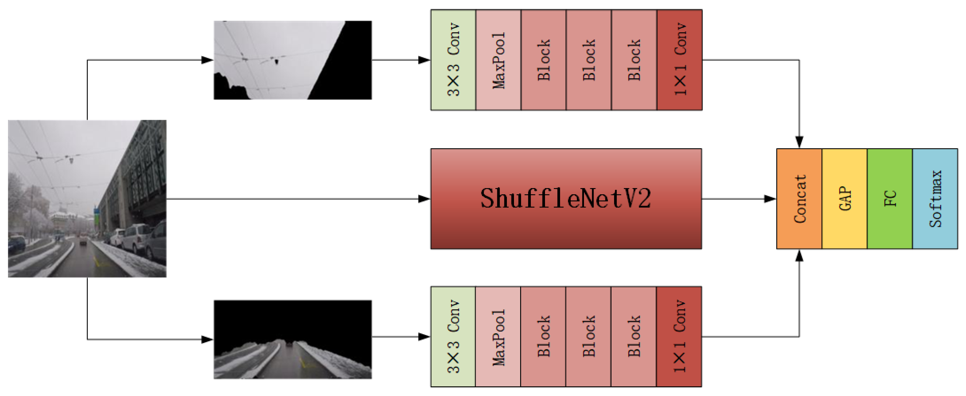
Based on this analysis, we propose a lightweight three-branch convolutional neural network. The input image is first segmented to extract the sky and road regions. Three CNN branches are then used to extract sky features, road features, and global features, respectively. These features are fused and passed to a classification layer for weather recognition. The structure of the three-branch CNN is shown in Figure 3.

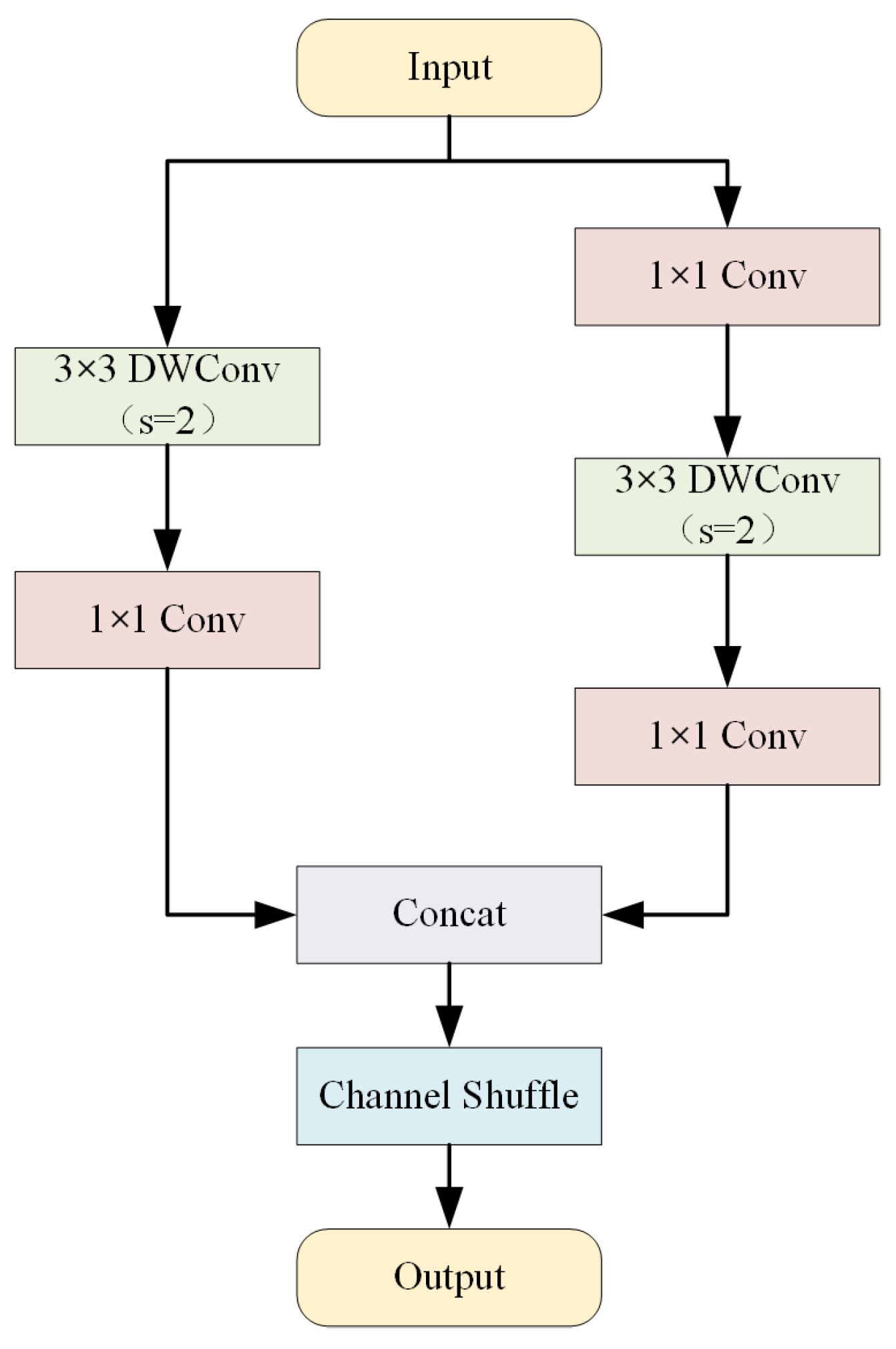
The main branch uses ShuffleNetV2_1x to extract global features from the input image of size 224 × 224 × 3, producing a feature map of size 7 × 7 × 512. To further enhance weather recognition, the semantically segmented sky and road regions are fed into the upper and lower branches to extract sky and road features, respectively. These two branches share the same structure, inspired by ShuffleNetV2. The input feature maps of size 224 × 112 × 3 undergo two downsampling steps via 3 × 3 convolution and max pooling, resulting in a feature map of size 56 × 56 × 24. Then, three Blocks are used for feature extraction, yielding a 7 × 7 × 464 feature map. The Block structure is shown in Figure 4. Finally, a 1 × 1 convolution adjusts the number of channels to 512. The sky and road region images are downsampled to 7 × 7 × 512 by these two branches. The feature maps from all three branches are concatenated along the channel dimension to form a fused feature map of size 7 × 7 × 1536. This fused feature is then passed to a classification layer consisting of global average pooling, fully connected layers, and a Softmax classifier to achieve weather recognition.

We constructed a custom weather image dataset based on Cityscapes dataset [23], Adverse Conditions Dataset with Correspondences(ACDC) [25] and our own collection, covering four weather classes: “Sunny”, “Rain”, “Fog”, and “Snow”. The dataset contained 5000 images in total, divided into 60% training, 20% validation, and 20% testing.

3.4. Vision-Based Road Recognition Method

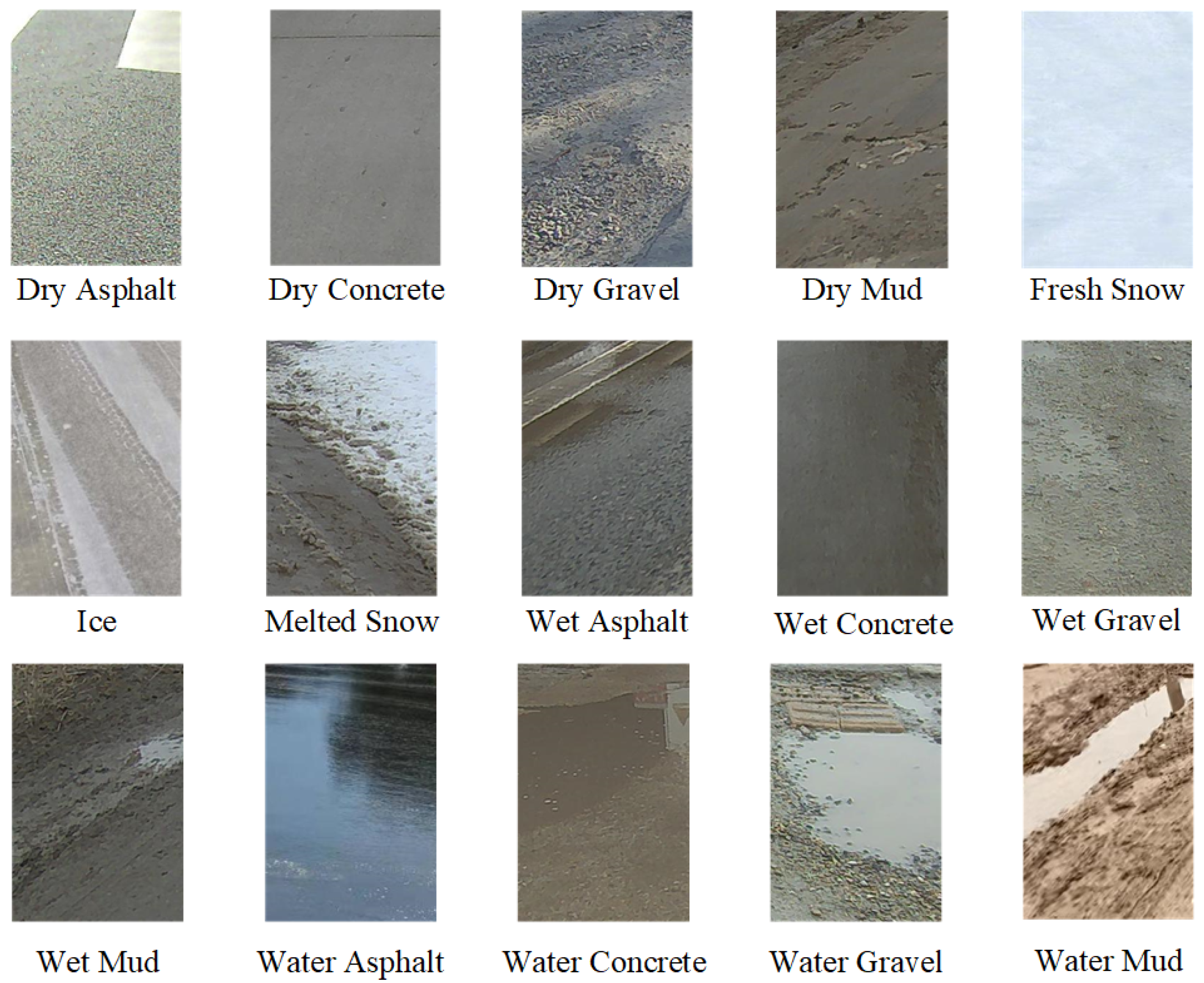
Many researchers have used neural networks for road image classification, but most rely on traditional public datasets. Conventional public vision datasets for Autonomous Driving vehicle perception focus on the overall environment rather than the road itself. The road surface often occupies a small area with low resolution, making fine-grained and accurate friction perception challenging. The RSCD dataset is a large-scale image dataset specifically designed for road condition perception [26]. As shown in the Figure 5, our method recognizes 15 road categories: “Dry Asphalt”, “Dry Concrete”, “Dry Gravel”, “Dry Mud”, “Fresh Snow”, “Ice”, “Melted Snow”, “Wet Asphalt”, “Wet Concrete”, “Wet Gravel”, “Wet Mud”, “Water Asphalt”, “Water Concrete”, “Water Gravel”, and “Water Mud”. A total of 885,800 labeled road images were used, with a split of 74% training, 8% validation, and 18% testing.

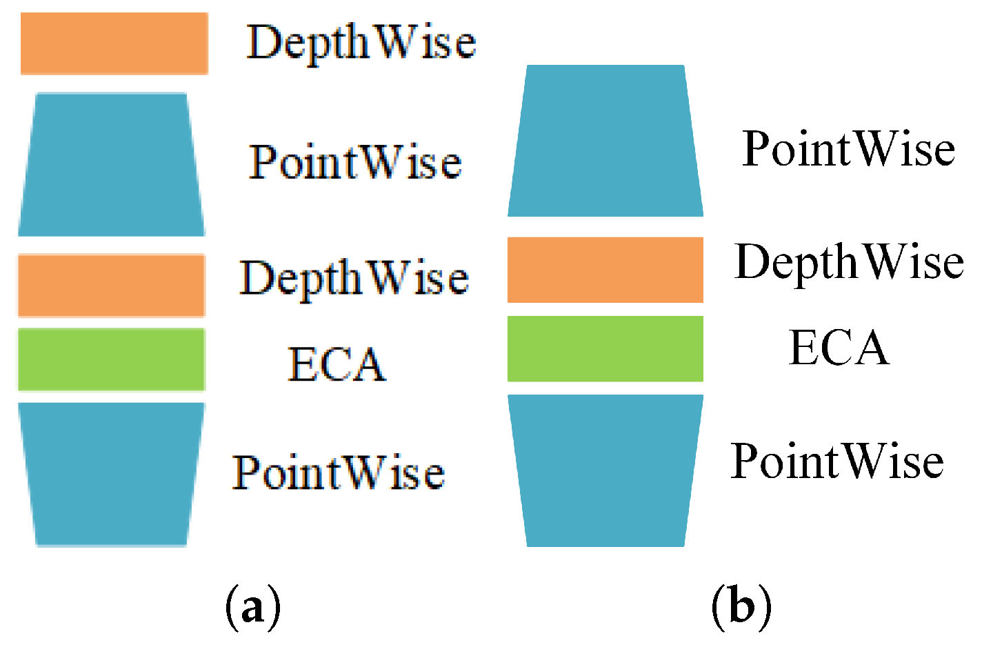
To meet the computational and power constraints of embedded automotive devices, we use the lightweight MobileNetV4-ConvSmall model as our core framework [27]. We further enhance its road recognition capability by incorporating an ECA mechanism. As shown in the

Table 1. Architecture of the enhanced MobileNetV4-ConvSmall.

Input	Block	ECA	Output Dim
224 × 224 × 3	Conv2D	-	32
112 × 112 × 32	FusedIB	-	32
56 × 56 × 32	FusedIB	-	64
28 × 28 × 64	ExtraDW	✔	96
14 × 14 × 96	IB	✔	96
14 × 14 × 96	IB	✔	96
14 × 14 × 96	IB	-	96
14 × 14 × 96	IB	-	96
14 × 14 × 96	ConvNext	-	96
14 × 14 × 96	ExtraDW	✔	128
7 × 7 × 128	ExtraDW	✔	128
7 × 7 × 128	IB	✔	128
7 × 7 × 128	IB	-	128
7 × 7 × 128	IB	-	128
7 × 7 × 128	IB	-	128
7 × 7 × 128	Conv2D	-	960
7 × 7 × 960	Avgpool	-	960
1 × 1 × 960	Conv2D	-	1280
1 × 1 × 1280	Conv2D	-	1000

, we improve the latter part of MobileNetV4-ConvSmall by integrating ECA into three ExtraDW blocks and three Inverted Bottleneck (IB) blocks, effectively increasing the model’s ability to focus on channel information while maintaining low computational complexity.

The improved Universal Inverted Bottleneck (UIB) structure is illustrated in the Figure 6. The ECA attention module is inserted before the last pointwise convolution. The two depthwise convolutions are optional. The ExtraDW block increases network depth and receptive field at low cost, while the Inverted Bottleneck (IB) performs spatial mixing on expanded feature activations to enhance model capacity at a higher computational cost.

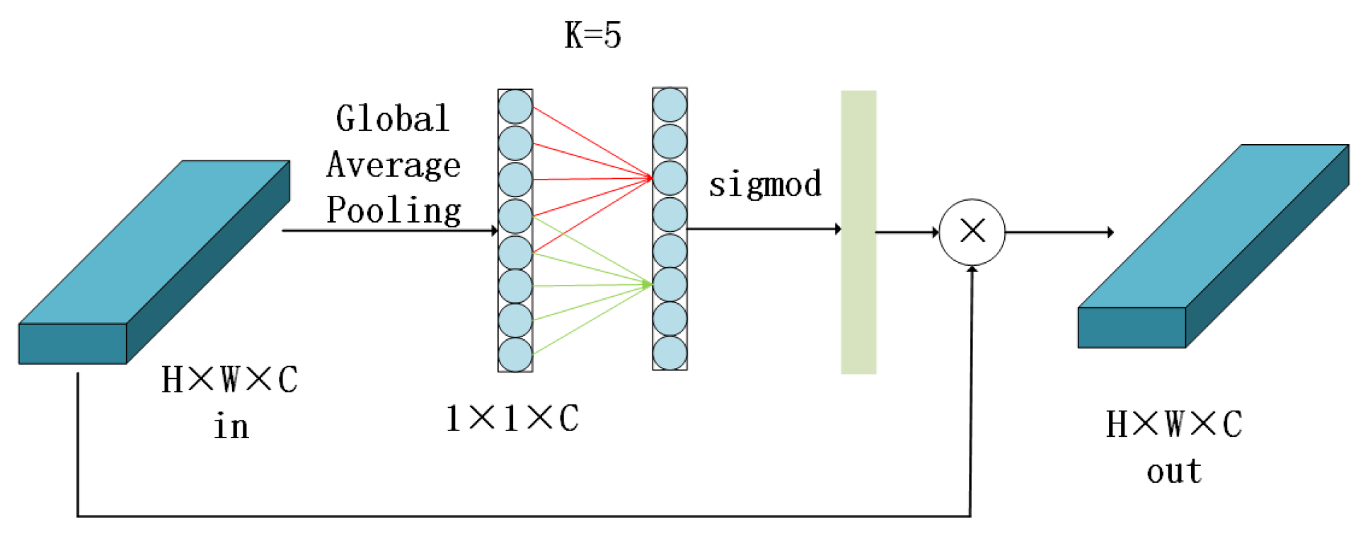
As shown in Figure 7, ECA efficiently captures local cross-channel interactions using 1D convolution. It first applies global average pooling to the input feature map, followed by a 1D convolution with kernel size K. A Sigmoid activation then maps the weights of each channel to the range [0, 1]. Finally, the weighted features are multiplied with the original input to produce the output feature map.

3.5. TRFC Fusion Estimation Based on Weather and Road Condition Information

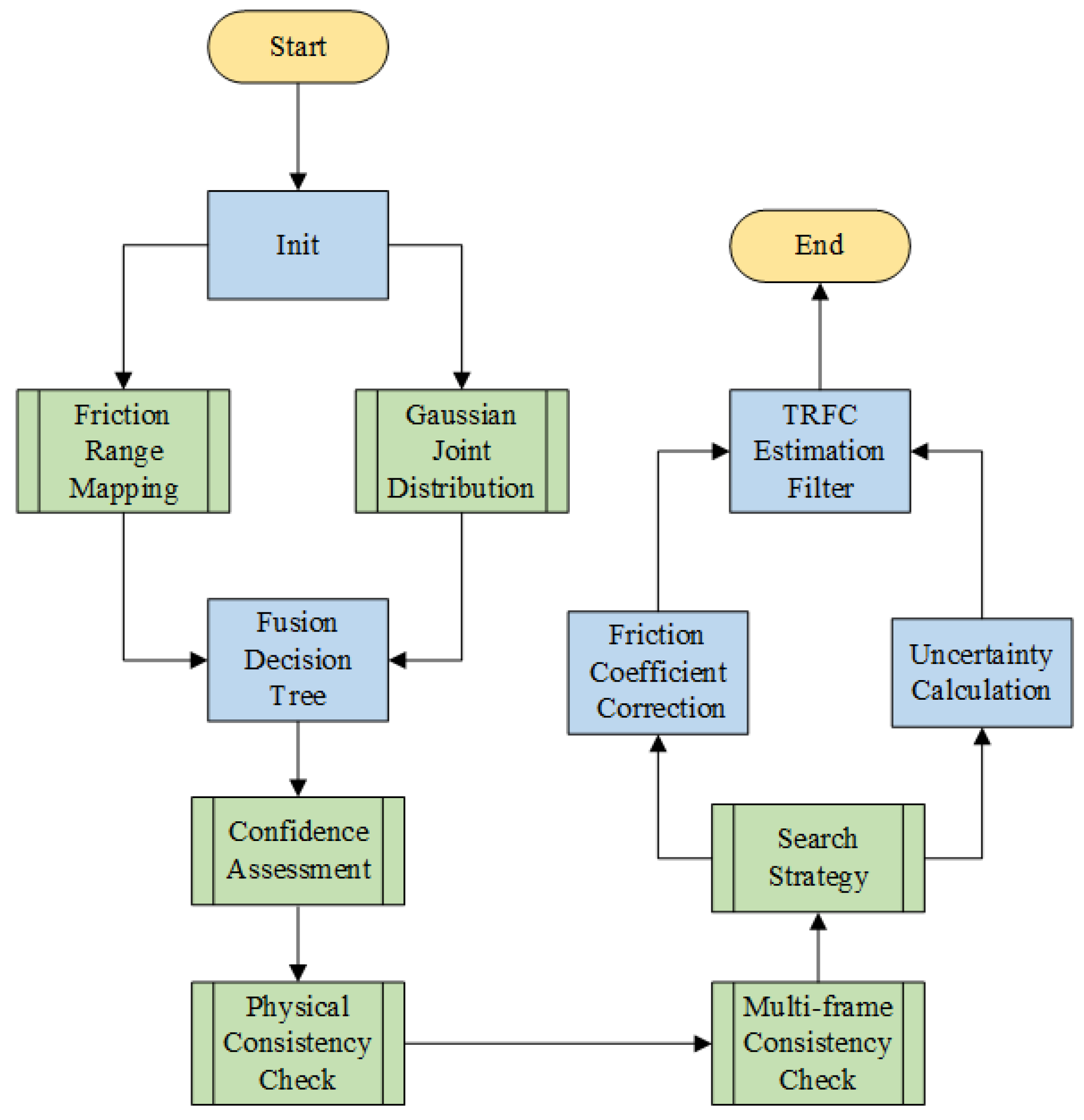
As illustrated in the algorithm flowchart (Figure 8), this paper proposes a TRFC fusion estimation method that integrates road classification and weather classification information to estimate the current road surface friction coefficient. The core of the method comprises several key processes: Gaussian probability modeling, a fusion decision tree, uncertainty calculation, filter update, and friction correction.

3.5.1. Gaussian Kernel-Based Initial Estimation of TRFC

The neural network can infer 15 road types and 4 weather types; however, this information cannot be directly used as the TRFC output. Therefore, we established a mapping relationship between the network outputs and TRFC values based on publicly available experimental data [14,28,29,30,31]. The typical TRFC ranges for some road and weather types are shown in

Table 2. Table of typical TRFC ranges corresponding to weather conditions.

Type	Upper	Down
Sunny	0.9	0.6
Rain	0.65	0.35
Fog	0.7	0.4
Snow	0.4	0.1

and

Table 3. Table of typical TRFC ranges corresponding to road types.

Type	Upper	Down
Dry Asphalt	0.9	0.7
Dry Concrete	0.9	0.7
Wet Asphalt	0.7	0.4
Water Asphalt	0.4	0.2
Fresh Snow	0.25	0.1
Ice	0.1	0.05

, respectively.

The actual TRFC is influenced by factors such as road conditions and vehicle dynamic states, and is not a constant value. To obtain a closer approximation of the true TRFC, a Gaussian distribution is modeled for each category output by the neural network. The kernel function is given by Equation (1), where the mean ${\mu }_{mj}$ is the midpoint of the prior range for that category, i.e., ${\displaystyle \frac{uppe{r}_j+dow{n}_j}{2}}$ and the standard deviation ${\sigma }_j$ is set to one-quarter of the range to ensure that most samples fall within the prior interval.

$$N_f\left(\mu \right)={\displaystyle \frac{1}{\sqrt{2\pi }{\sigma }_j}}exp\left(-{\displaystyle \frac{{(\mu -{\mu }_{mj})}^2}{2{\sigma }_j^2}}\right)$$

(1)

The classification results of the neural network for both road and weather are not deterministic values, but rather probability distributions. Therefore, as shown in Equation (2), a Gaussian Mixture Model is constructed based on the classification probability vector and the Gaussian distribution of each category. This model represents the overall probability density of the friction coefficient given the current classification results.

$$p\left(\mu \right)=\sum _j{w}_j·N_j\left(\mu \right)$$

(2)

where $w_j$ is the probability assigned to class j by the classification network. The initial friction coefficient estimate ${\mu }_i$ is obtained by maximizing this mixture probability density function (PDF). To find the global maximum of the mixture PDF, a fine-grid search algorithm is employed. This algorithm creates a dense, uniformly discretized grid over a defined domain $[{\mu }_{min},{\mu }_{max}]$ and computes the density value at each grid point to locate the maximum. First, a uniform grid comprising M points is defined:

$$\mathcal{G}={\mu }_1,{\mu }_2,\dots ,{\mu }_M\mathrm{where}{\mu }_k={\mu }_{min}+(k-1)·{\displaystyle \frac{{\mu }_{max}-{\mu }_{min}}{M-1}},k=1,2,\dots ,M$$

(3)

For each point ${\mu }_k\in \mathcal{G}$ in the grid, compute its mixture probability density:

$$p\left({\mu }_k\right)=\sum _{j=0}^{N-1}{w}_j·{\displaystyle \frac{1}{\sqrt{2\pi }{\sigma }_j}}exp\left(-{\displaystyle \frac{{({\mu }_k-{\mu }_{mj})}^2}{2{\sigma }_j^2}}\right)$$

(4)

By comparing the density values at all grid points, find the point that maximizes $p\left({\mu }_k\right)$:

$$k^{*}=arg\underset{k\in 1,2,\dots ,M}{max}p\left({\mu }_k\right)$$

(5)

The corresponding grid point $k^{*}$ is the resulting initial estimate of the friction coefficient, denoted as ${\mu }_i$.

3.5.2. Fusion Decision Tree

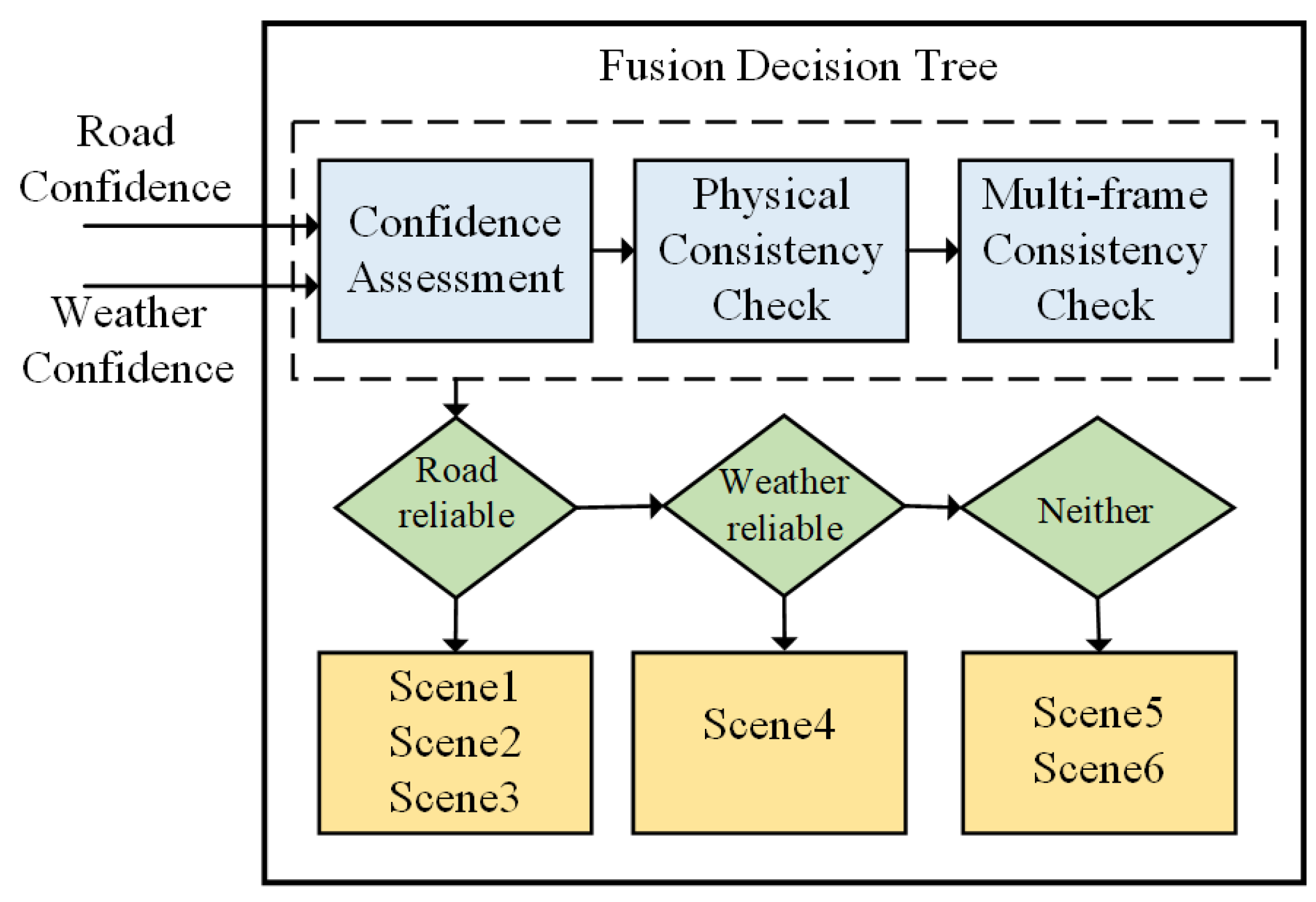
As shown in Figure 9, to effectively utilize both weather and road recognition information, we propose a rule-based multi-modal fusion decision tree. This framework integrates physical consistency check (e.g., rain should not coincide with a dry road surface) and multi-frame consistency check (to mitigate single-frame misdetections). A total of six primary fusion scenarios are defined. The most suitable strategy is dynamically selected based on real-time confidence assessment, ultimately yielding a robust estimation policy.

Multi-frame consistency check employs a sliding window to detect stability across consecutive frames by computing both categorical variance and confidence stability. The former quantifies fluctuations in the number of categories, while the latter measures variations in confidence levels:

$$\mathrm{class\_variance}={\displaystyle \frac{\mathrm{unique\_classes}}{N}}$$

(6)

$${\mu }_{\mathrm{conf}}={\displaystyle \frac{1}{N}}\sum _{i=1}^N{c}_i$$

(7)

$${\sigma }_{\mathrm{conf}}=\sqrt{{\displaystyle \frac{1}{N-1}}\sum _{i=1}^N{(c_i-{\mu }_{\mathrm{conf}})}^2}$$

(8)

where N denotes the number of historical frames and unique_classes represents the number of distinct classes observed in these frames. By evaluating whether these metrics exceed predefined thresholds, the system determines whether to trust the current estimation.

Specific triggering conditions and corresponding operational scenarios are summarized in

Table 4. Table of estimation strategy.

Scene	RC	WC	PC	RMFC	WMFC	Strategy
Scene1	>High	>High	TRUE	TRUE	TRUE	Road + Weather Adjust
Scene2	>High	<Low	-	TRUE	-	Road
Scene3	>High	<Low	FALSE	TRUE	TRUE	Road
Scene4	<Low	>High	-	-	TRUE	Weather
Scene5(1)	<Low	-	-	-	FALSE	Historical Value
Scene5(2)	-	<Low	-	FALSE	-	Historical Value
Scene5(3)	-	-	-	FALSE	FALSE	Historical Value
Scene6	>Low & <High	>Low & <High	TRUE	TRUE	TRUE	Weighted Average

. “RC”, “WC”, “PC”, “RMFC”, and “WMFC” denote “Road Confidence”, “Weather Confidence”, “Physical Consistency”, “Road Multi-Frame Consistency”, and “Weather Multi-Frame Consistency”, respectively. The fusion decision tree reflects the high robustness of the system. Its core principle is to prioritize highly confident information; when information conflicts or is deemed unreliable, multi-frame consistency checking is introduced as an arbitration mechanism; in cases where both road and weather information are unreliable, the system maintains stability by inheriting historical values from the filter.

Given the complexity of real-world driving conditions, special strategies have been designed for particular scenarios to ensure accurate friction estimation by the filter. For instance, when a water truck wets the road on a sunny day, resulting in a physically inconsistent condition, the system falls into Scenario 3 and adopts an estimation strategy that prioritizes road information.

As summarized in

Table 5. TRFC correction table.

Strategy	${\mathit{\mu }}_{\mathit{r}}$
Road + Weather Adjust	${\mu }_r={\mu }_{i\_road}(1+\mathrm{adjustment})$
Road	${\mu }_r={\mu }_{i\_road}$
Weather	${\mu }_r={\mu }_{i\_weather}$
Historical Value	TRFC Value from the Previous Time Step
Weighted Average	${\mu }_r=w_{road}{\mu }_{i\_road}+w_{weather}{\mu }_{i\_weather}$

, the initial friction estimate ${\mu }_i$ is adjusted according to the fusion strategy to obtain a revised value ${\mu }_r$.

3.5.3. Uncertainty Modeling and Filtering Estimator

To quantify the uncertainty of the probability distribution output by the neural network, we employ information entropy as a measure:

$$H=-\sum _{j=0}^{N-1}{p}_j·log\left(p_j\right)$$

(9)

where N denotes the total number of categories (15 for road types and 4 for weather conditions), j is the class index, and $p_j$ represents the probability of the j-th class. The entropy is then normalized to obtain an uncertainty measure $uc$ within the range $[0,1]$:

$$uc={\displaystyle \frac{H}{H_{max}}}={\displaystyle \frac{-{\sum }_{j=0}^{N-1}{p}_j·log\left(p_j\right)}{log\left(N\right)}}$$

(10)

After obtaining the uncertainty measures for road and weather, denoted as $u{c}_{road}$ and $u{c}_{weather}$ respectively, they are weighted and combined according to the strategy provided by the fusion decision tree to yield a final overall uncertainty measure $u{c}_{total}$. A piecewise linear function is employed to map $u{c}_{total}$ to the gain control factor $K_u$ for the filter:

$$K_u\left(uc\right)=\left\{\begin{array}{cc}{K}_{u_{max}}=1.0,\hfill & uc\le 0\hfill \\ 1-uc,\hfill & 0<uc\le 0.3\hfill \\ 1.3-2uc,\hfill & 0.3<uc\le 0.5\hfill \\ 2.8-5uc,\hfill & 0.5<uc<0.55\hfill \\ K_{u_{min}}=0.05,\hfill & uc\ge 0.55\hfill \end{array}\right.$$

(11)

Finally, the dynamic gain control factor $K_u$ is incorporated into the TRFC estimation filter update equation to obtain the friction coefficient estimate at the current time step ${\widehat{\mu }}_t$:

$${\widehat{\mu }}_t={\widehat{\mu }}_{t-1}+K_u({\mu }_{r,i}-{\widehat{\mu }}_{t-1})$$

(12)

where ${\widehat{\mu }}_{t-1}$ represents the estimated value from the previous time step.

4. Experiments

4.1. Training and Testing Results of the Image Segmentation and Recognition Network

The mean Intersection over Union (MIoU) is an important metric for evaluating the performance of semantic segmentation networks, particularly suited for comprehensive accuracy assessment in multi-class segmentation tasks. It is calculated as the average of the Intersection over Union (IoU) values for each individual class. As shown in Equation (13), the numerator represents the intersection between the ground truth and predicted values, while the denominator represents their union, with N denoting the number of segmentation categories.

$$MIoU={\displaystyle \frac{1}{N}}\sum _{i=1}^N{\displaystyle \frac{TP}{FN+FP+TP}}$$

(13)

The DeepLabV3+ model was trained for a total of 100 epochs using the Adam optimizer. During the first 50 epochs, the backbone was frozen to stabilize low-level feature extraction, and in the subsequent 50 epochs, all layers were unfrozen for fine-tuning. After training, the DeepLabV3+ model achieves an MIoU of 90.95%, which meets the requirements for subsequent weather and road recognition networks.

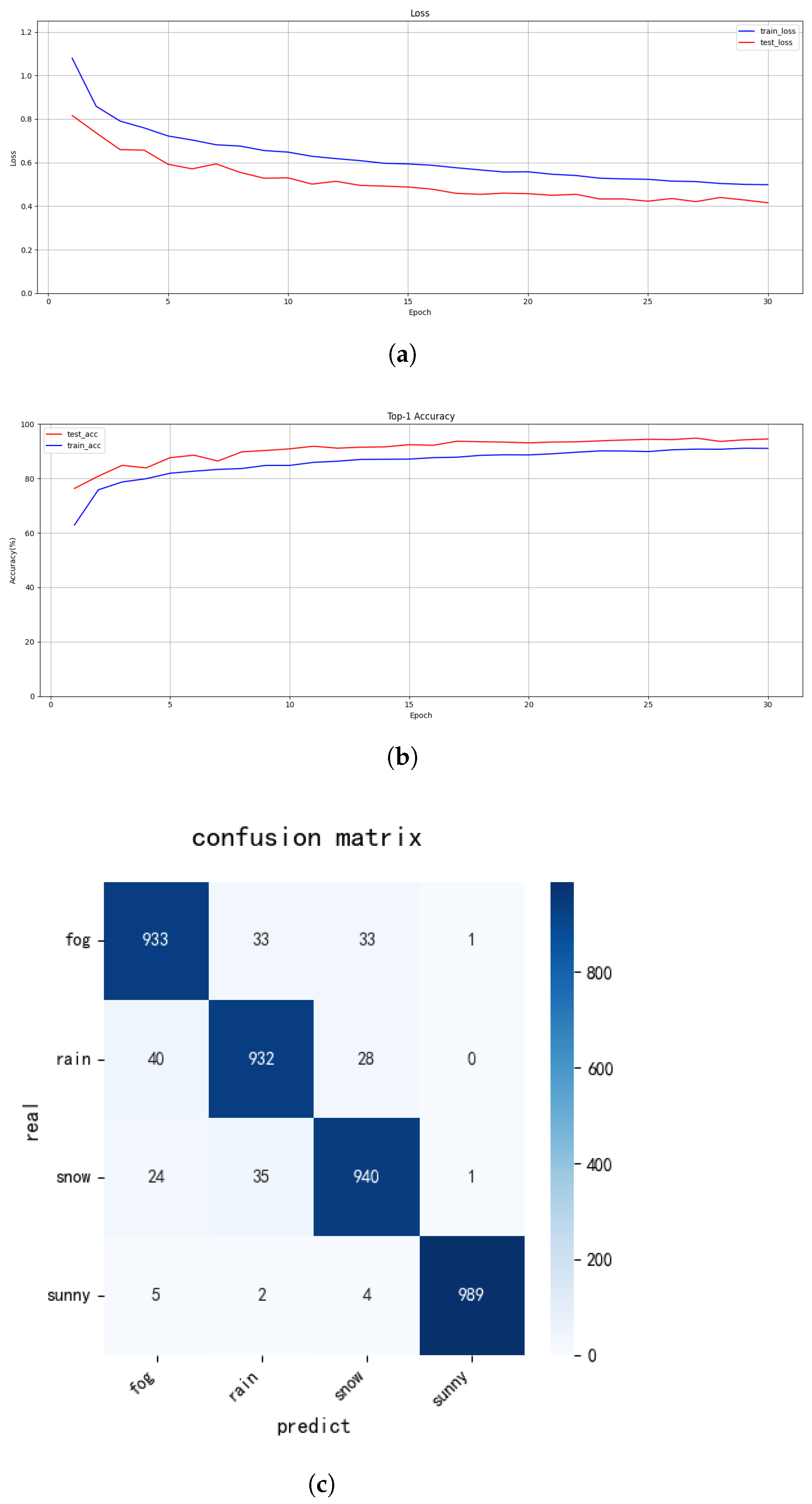
For the weather recognition network, the training was configured with 30 epochs using the Adam optimizer. Since the upper and lower branches of the three-branch composite convolutional neural network did not have corresponding pre-trained weights, only transfer learning was applied to the backbone network. The loss and top-1 accuracy curves of the weather recognition network are shown in the Figure 10. As the number of epochs increased, the network gradually converged, reaching the highest accuracy of 94.85% on the test set at the 27th epoch. Further confusion matrix analysis of the trained model revealed that sunny conditions were predicted with the highest accuracy and were least likely to be misclassified into other weather categories. However, Rain, Fog, and Snow were often confused with each other, primarily due to their similar overall dark and grayish tones.

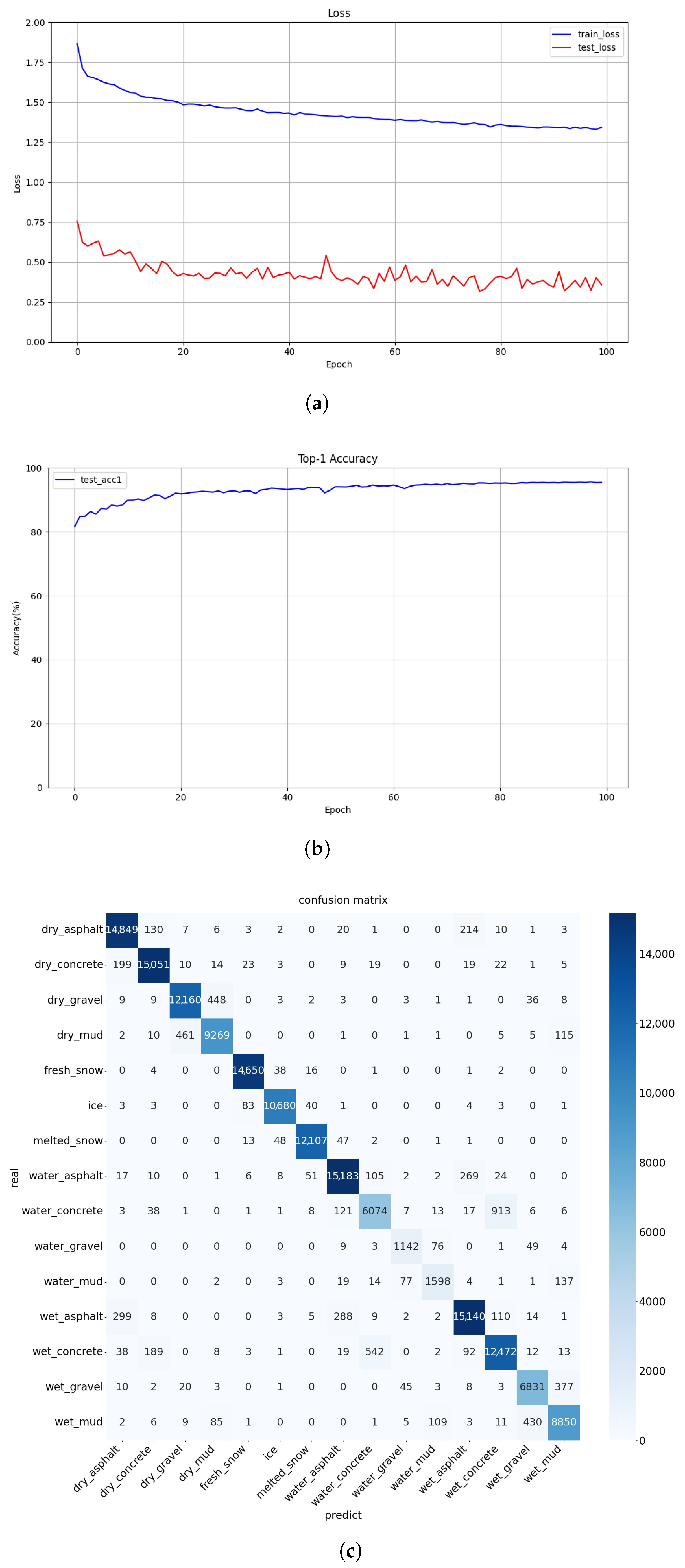
For the road recognition network, the training was set to 100 epochs using the AdamW optimizer with a 5-epoch warm-up period. Given the relatively large dataset, a pre-trained model was employed to accelerate convergence. The loss and top-1 accuracy curves of Enhanced MobileNetV4-ConvSmall are shown in the Figure 11, both indicating consistent trends throughout the training process. The network approached convergence around the 50th epoch, with the peak accuracy of 95.63% achieved at the 97th epoch.

Enhanced MobileNetV4-ConvSmall was designed to recognize 15 types of road surfaces, and the confusion matrix served as an important metric for evaluating classification performance, as illustrated in Figure 11c. The vertical axis of the matrix represents the actual number of samples per class, while the horizontal axis corresponds to the predicted class labels. The diagonal entries indicate the number of correctly classified images. Although most categories were accurately recognized, the network exhibited slightly reduced performance in distinguishing between wet_concrete and water_concrete, mainly due to the ambiguous visual boundaries between “wet” and “water” conditions.

Table 6. Performance comparison between MNV4-C-S and E-MNV4-C-S.

Model Name	Precision (%)	Recall (%)	F1-Score (%)	Model Size (M)
MNV4-C-S	94.77	94.78	94.76	3.8
E-MNV4-C-S	95.64	95.63	95.63	3.81

presents a performance comparison between the MobileNetV4-ConvSmall and the Enhanced MobileNetV4-ConvSmall proposed in this study. With only a 0.26% increase in the number of parameters, the Precision improved from 94.77% to 95.64%. The experimental results demonstrate that incorporating the ECA attention mechanism effectively enhances the model’s performance.

4.2. TRFC Fusion Estimation Method

To validate the effectiveness of the fusion recognition method, we conducted ablation experiments to compare the robustness of the fusion method against a vision-only approach that relies solely on road image recognition. The onboard camera captured driving video at 8 FPS. Testing scenarios included four conditions: “Sunny Weather with Unknown Road Surface,” “Rainy Weather with Asphalt Road Surface,” “Fog Weather with Asphalt Road Surface”, and “Transition Road Surface.”

4.2.1. Constant Road Surface

(1)

Sunny Weather with Unknown Road Surface

The “Sunny Weather with Unknown Road Surface” was selected to test the generalization capability of the proposed method. In this case, the vehicle entered a brick-paved road that was not included in the RSCD training dataset. This scenario effectively evaluates the method’s robustness to unseen road types, where vision-only methods typically fail to produce stable estimations.

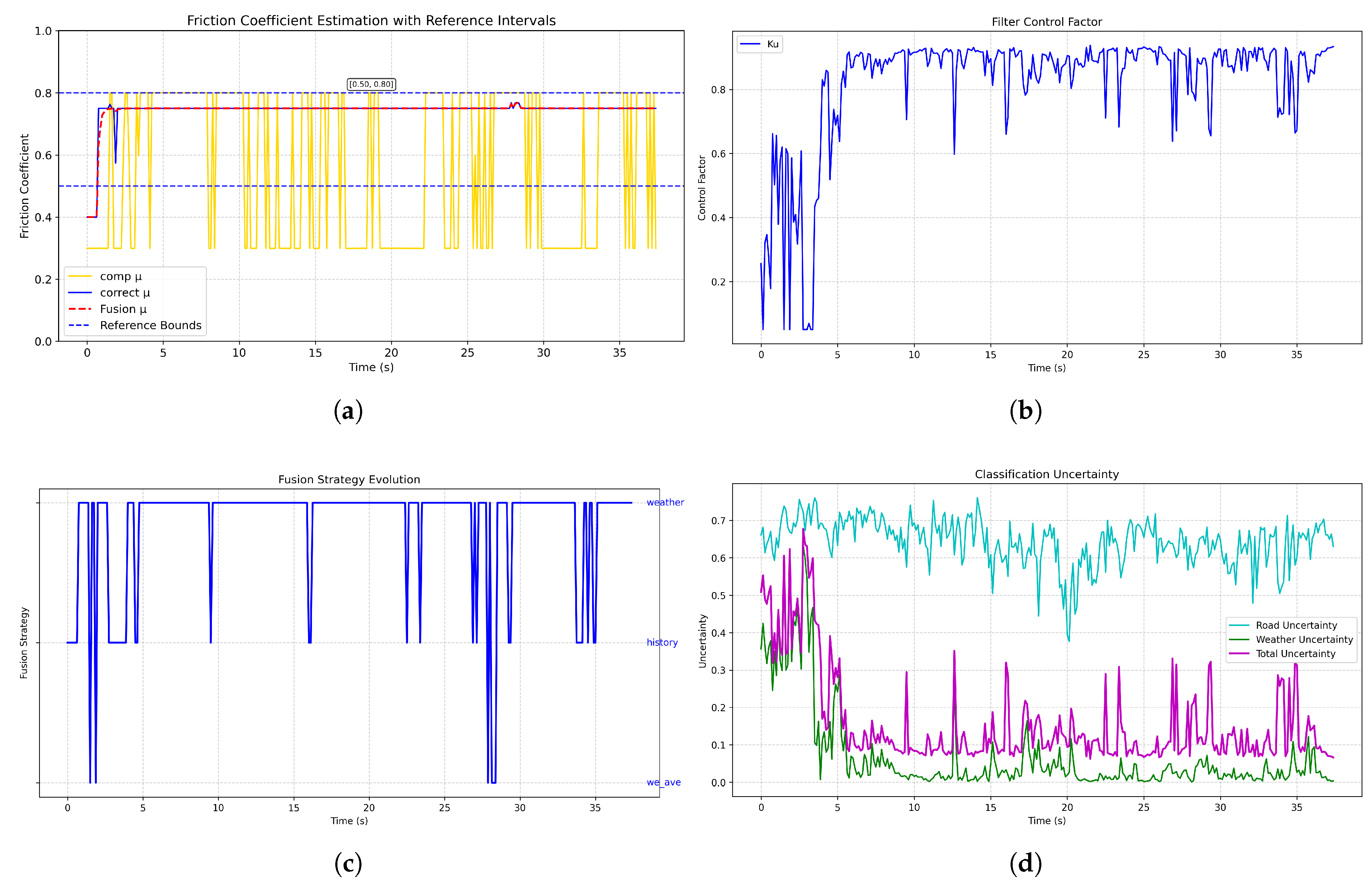
Figure 12 presents the results of the ablation experiments: (a) TRFC estimation results, (b) filter control factor, (c) fusion strategy, and (d) uncertainty of weather and road recognition results.

In subfigure (a), the Golden yellow line represents the recognition results obtained using the method proposed in Reference [32], which also employed the RSCD dataset for road type recognition. Since this specific road type was not included in the RSCD dataset, the method fails to produce stable road identification results, causing the TRFC estimates to oscillate frequently between 0.3 and 0.8. In contrast, owing to the fusion algorithm proposed in this paper, the final TRFC estimation ${\widehat{\mu }}_t$—represented by the red dashed line—remain stable. The blue line denotes the corrected TRFC value ${\mu }_r$, obtained by applying the fusion decision tree to reconcile road and weather information. After being processed by the uncertainty filter with a dynamic gain control factor $K_u$, the corrected value ${\mu }_r$ yields the final TRFC estimation ${\widehat{\mu }}_t$.

The stability of the TRFC estimation (red dashed line in Figure 12a) ensures that the control system receives consistent and reliable friction information. This prevents abrupt control variations that might occur under oscillating estimations, leading to smoother torque or braking control. Consequently, vehicle stability and passenger comfort are improved, which is particularly critical for safety functions such as ADAS and ABS.

As shown in subfigure (d), the blue solid line represents the uncertainty output from the road type recognition neural network. When driving on an unknown road surface, the road recognition uncertainty is very high, while the weather is stably identified as “Sunny”. Consequently, the low uncertainty in weather recognition leads the fusion decision tree in subfigure (c) to predominantly trust the weather recognition outcome.

Between 0–4 s, due to obstruction from buildings, the weather recognition result fluctuates, causing corresponding oscillations in the corrected value ${\mu }_r$. However, owing to the high overall uncertainty, the dynamic filter gain control factor suppresses drastic changes in the friction coefficient. After the algorithm converges, the friction coefficient stabilizes between 0.75 and 0.77, which aligns with the typical range for dry road surfaces under sunny conditions. This demonstrates that the fusion algorithm can provide effective estimates even on unknown road surfaces, exhibiting high robustness.

(2)

Rainy Weather with Asphalt Road Surface

Under rainy asphalt conditions, the road recognition network’s accuracy decreases due to confusion between wet asphalt and water-accumulated asphalt surfaces. This leads to misclassification between “Wet Asphalt” and “Water Asphalt”. Thus, as shown in Figure 13, the road-only method yields estimates oscillating between 0.3 and 0.55. However, after processing by the fusion decision tree and the uncertainty-aware filter, the estimated value stabilizes between 0.52 and 0.55, which is consistent with typical friction ranges for rainy driving conditions.

(3)

Fog Weather with Asphalt Road Surface

To evaluate the performance of the proposed method under hard conditions, we conducted an experiment in the “Fog Weather with Asphalt Road Surface” scenario. The results are shown in Figure 14. Fog significantly reduces camera visibility and prevents clear capture of road surface details; consequently, road-only method fail to correctly identify the road type. In subfigure (a), the green line denotes the road-only method, which is unable to produce meaningful estimates throughout the sequence, while the red dashed line denotes the proposed fusion method. The fusion method, by relying on weather recognition, is able to provide estimations that fall within a reasonable range. However, because the foggy images do not allow reliable inference of road wetness, the method cannot determine precise wetness-related properties and therefore cannot produce highly accurate TRFC value—a limitation common to most vision-based approaches.This limitation motivates future research to extend the approach by incorporating non-visual modalities (e.g., vehicle dynamics) and image-enhancement techniques (e.g., dehazing or thermal imaging) to improve the accuracy of friction estimation under severe visibility degradation.

4.2.2. Transition Road Surface

During driving, the vehicle may transition between different road surfaces, which can affect the TRFC. We tested the proposed fusion method on a transition from “Dry Asphalt” to “Dry Mud” road. As shown in Figure 15, at the 14-s mark, the road surface changes from “Dry Asphalt” to “Dry Mud”. The fusion method enables the estimated friction coefficient to rapidly converge to the range typical for mud roads.

4.2.3. Error Metric Comparison

Table 7. Table of the error metric comparison.

Method	Case	In-Range Accuracy (%)	Mean Deviation	Root Mean Square Error
Our Paper	Unknown Road	98.00	0.0924	0.1049
Ref. [32]	Unknown Road	23.00	−0.0912	0.2646
Our Paper	Fog	98.00	−0.1031	0.1052
Road Only	Fog	0.33	−0.3491	0.3504

summarizes a quantitative comparison between our proposed fusion estimator and two baselines under two conditions (Unknown Road and Fog). To evaluate the performance of the proposed TRFC estimation method, we computed three error metrics for quantitative assessment: In-Range Accuracy: Percentage of estimates within the reference interval, indicating physical plausibility. Mean Deviation: Average deviation from the interval midpoint, reflecting estimation bias. Root Mean Square Error (RMSE): Root mean square deviation from the midpoint, measuring estimation precision.

As shown in Table 7, for the “Sunny Weather with Unknown Road Surface” scenario our method achieves an In-Range Accuracy of 98.00%, a Mean Deviation of +0.0924, and an RMSE of 0.1049, whereas baseline Ref. [32] attains only 23.00% In-Range Accuracy with a negative Mean Deviation (−0.0912) and a substantially larger RMSE (0.2646). For the “Fog Weather with Asphalt Road Surface” case the proposed fusion approach again yields high In-Range Accuracy (98.00%) with Mean Deviation (−0.1031) and RMSE (0.1052). In contrast, a road-only method under fog fails to provide physically plausible estimates (In-Range Accuracy 0.33%, Mean Deviation −0.3491, RMSE 0.3504).

These results indicate that the proposed fusion scheme produces estimates that are both more consistent with physically plausible friction ranges and quantitatively closer to the reference values than the considered baselines—especially in hard or previously unseen conditions (unknown road types and low-visibility scenarios).

5. Conclusions

To address the poor generalization capability of vision-only methods in TRFC estimation, this paper proposes a novel TRFC estimation framework that fuses weather and road image information. By employing semantic segmentation to extract sky and road features separately, and incorporating an improved lightweight MobileNetV4 along with a three-branch convolutional network, the system achieves high-precision weather and road type recognition while maintaining computational efficiency. Furthermore, through a fusion decision tree and an uncertainty modeling mechanism, the system dynamically adjusts the estimation strategy to effectively handle conflicts or unreliable recognition results, significantly enhancing robustness and adaptability.

Ablation experiments demonstrate the effectiveness of the proposed fusion method under various complex scenarios, including unknown road surfaces and transition roads. Compared to single-modality road recognition methods, the proposed approach significantly reduces estimation oscillation and improves convergence speed and stability, thereby providing more reliable environmental perception for intelligent driving systems.

Quantitatively, the proposed fusion method consistently delivers estimates that fall within physically plausible friction ranges and outperform vision-only baselines. As summarized in Table 7, for the “Sunny Weather with Unknown Road Surface” scenario the method attains an in-range accuracy of 98.00%, a mean deviation of +0.0924, and an RMSE of 0.1049. For the “Fog Weather with Asphalt Road Surface” case it achieves 98.00% in-range accuracy, a mean deviation of −0.1031, and an RMSE of 0.1052. These results indicate that fusing weather information and applying uncertainty-aware filtering substantially improves estimation robustness in challenging and previously unseen conditions.

However, we also note some limitations. Under extreme low-visibility conditions (e.g., dense fog, night driving or dirty lens), visual signals may be insufficient to determine road surface details, which limits the attainable accuracy of TRFC estimates—a limitation common to vision-based methods.

Future work will focus on overcoming these limitations by integrating non-visual modalities (e.g., vehicle-dynamics modeling) and applying image-enhancement techniques (e.g., dehazing or thermal imaging) to achieve improved performance at minimal additional cost. These extensions are expected to further enhance TRFC estimation accuracy and provide better environmental perception for ADAS and AD systems.

References

1. Bei, Z.; Chen, X.; Zhao, W.; Wang, C. A novel algorithm for tire-road friction coefficient estimation using adaptive backpropagation neural network. J. Phys. Conf. Ser. 2024, 2832, 012018. [Google Scholar] [CrossRef]
2. Wang, C.; Wang, Z.; Zhang, Z.; Liu, J.; Li, W.; Wu, Y.; Li, X.; Yu, H.; Cao, D. Integrated post-impact planning and active safety control for autonomous vehicles. IEEE Trans. Intell. Veh. 2023, 8, 2062–2076. [Google Scholar] [CrossRef]
3. Wang, S.F.; Liang, Q.W.; Liu, Z.; Zhang, J.Y. Research on collision avoidance control of intelligent vehicles based on MSTUKF road adhesion coefficient identification. Adv. Transp. Stud. 2022, 58, 245. [Google Scholar]
4. Korayem, A.H.; Khajepour, A.; Fidan, B. A review on vehicle-trailer state and parameter estimation. IEEE Trans. Intell. Transp. Syst. 2021, 23, 5993–6010. [Google Scholar] [CrossRef]
5. Huang, Z.; Fan, X. A review on estimation of vehicle tyre-road friction. Int. J. Heavy Veh. Syst. 2024, 31, 49–86. [Google Scholar] [CrossRef]
6. Quan, Z.; Li, B.; Bei, S.; Sun, X.; Xu, N.; Gu, T. Tire-road friction coefficient estimation method design for intelligent tires equipped with PVDF piezoelectric film sensors. Sens. Actuators A Phys. 2023, 349, 114007. [Google Scholar] [CrossRef]
7. Zou, Z.; Zhang, X.; Zou, Y.; Lenzo, B. Tire-road friction coefficient estimation method design for intelligent tires equipped with three-axis accelerometer. SAE Int. J. Veh. Dyn. Stab. NVH 2021, 5, 249–258. [Google Scholar] [CrossRef]
8. Yu, M.; Xu, X.; Wu, C.; Li, S.; Li, M.; Chen, H. Research on the prediction model of the friction coefficient of asphalt pavement based on tire-pavement coupling. Adv. Mater. Sci. Eng. 2021, 2021, 6650525. [Google Scholar] [CrossRef]
9. Han, Y.; Lu, Y.; Liu, J.; Zhang, J. Research on tire/road peak friction coefficient estimation considering effective contact characteristics between tire and three-dimensional road surface. Machines 2022, 10, 614. [Google Scholar] [CrossRef]
10. Ye, J.; Zhang, Z.; Jin, J.; Su, R.; Huang, B. Estimation of tire-road friction coefficient with adaptive tire stiffness based on RC-SCKF. Nonlinear Dyn. 2024, 112, 945–960. [Google Scholar] [CrossRef]
11. Tao, S.; Ju, Z.; Li, L.; Zhang, H.; Pedrycz, W. Tire road friction coefficient estimation for individual wheel based on two robust pmi observers and a multilayer perceptron. IEEE Trans. Veh. Technol. 2024, 73, 12530–12541. [Google Scholar] [CrossRef]
12. Zhang, Z.; Zheng, L.; Wu, H.; Zhang, Z.; Li, Y.; Liang, Y. An estimation scheme of road friction coefficient based on novel tyre model and improved SCKF. Veh. Syst. Dyn. 2022, 60, 2775–2804. [Google Scholar] [CrossRef]
13. Wang, Y.; Yin, G.; Hang, P.; Zhao, J.; Lin, Y.; Huang, C. Fundamental estimation for tire road friction coefficient: A model-based learning framework. IEEE Trans. Veh. Technol. 2024, 74, 481–493. [Google Scholar] [CrossRef]
14. Zhao, S.; Zhang, J.; Jiang, Y.; He, C.; Han, J. Tire-road friction coefficients adaptive estimation through image and vehicle dynamics integration. Mech. Syst. Signal Process. 2025, 224, 112039. [Google Scholar] [CrossRef]
15. Xia, J.; Xuan, D.; Tan, L.; Xing, L. ResNet15: Weather recognition on traffic road with deep convolutional neural network. Adv. Meteorol. 2020, 2020, 6972826. [Google Scholar] [CrossRef]
16. Xiao, H.; Zhang, F.; Shen, Z.; Wu, K.; Zhang, J. Classification of weather phenomenon from images by using deep convolutional neural network. Earth Space Sci. 2021, 8, e2020EA001604. [Google Scholar] [CrossRef]
17. Li, Z.; Li, Y.; Zhong, J.; Chen, Y. Multi-class weather classification based on multi-feature weighted fusion method. IOP Conf. Ser. Earth Environ. Sci. 2020, 558, 042038. [Google Scholar] [CrossRef]
18. Chen, L.; Qin, Z.; Bian, Y.; Hu, M.; Peng, X. Data-driven tire-road friction estimation for electric-wheel vehicle with data category selection and uncertainty evaluation. IEEE Trans. Ind. Electron. 2024, 72, 3048–3060. [Google Scholar] [CrossRef]
19. Leng, B.; Jin, D.; Xiong, L.; Yang, X.; Yu, Z. Estimation of tire-road peak adhesion coefficient for intelligent electric vehicles based on camera and tire dynamics information fusion. Mech. Syst. Signal Process. 2021, 150, 107275. [Google Scholar] [CrossRef]
20. Leng, B.; Jin, D.; Hou, X.; Tian, C.; Xiong, L.; Yu, Z. Tire-road peak adhesion coefficient estimation method based on fusion of vehicle dynamics and machine vision. IEEE Trans. Intell. Transp. Syst. 2022, 23, 21740–21752. [Google Scholar] [CrossRef]
21. Tian, C.; Leng, B.; Hou, X.; Xiong, L.; Huang, C. Multi-sensor fusion based estimation of tire-road peak adhesion coefficient considering model uncertainty. Remote Sens. 2022, 14, 5583. [Google Scholar] [CrossRef]
22. Guo, H.; Zhao, X.; Liu, J.; Dai, Q.; Liu, H.; Chen, H. A fusion estimation of the peak tire–road friction coefficient based on road images and dynamic information. Mech. Syst. Signal Process. 2023, 189, 110029. [Google Scholar] [CrossRef]
23. Cordts, M.; Omran, M.; Ramos, S.; Rehfeld, T.; Enzweiler, M.; Benenson, R.; Franke, U.; Roth, S.; Schiele, B. The Cityscapes dataset for semantic urban scene understanding. In Proceedings of the IEEE Conference on Computer Vision and Pattern Recognition, Las Vegas, NV, USA, 27–30 June 2016; pp. 3213–3223. [Google Scholar] [CrossRef]
24. Chen, L.C.; Zhu, Y.; Papandreou, G.; Schroff, F.; Adam, H. Encoder-decoder with atrous separable convolution for semantic image segmentation. In Proceedings of the European Conference on Computer Vision (ECCV), Munich, Germany, 8–14 September 2018; pp. 801–818. [Google Scholar] [CrossRef]
25. Sakaridis, C.; Dai, D.; Van Gool, L. ACDC: The adverse conditions dataset with correspondences for semantic driving scene understanding. In Proceedings of the IEEE/CVF International Conference on Computer Vision, Montreal, QC, Canada, 10–17 October 2021; pp. 10765–10775. [Google Scholar] [CrossRef]
26. Zhao, T.; Wei, Y. A road surface image dataset with detailed annotations for driving assistance applications. Data Brief 2022, 43, 108483. [Google Scholar] [CrossRef] [PubMed]
27. Qin, D.; Leichner, C.; Delakis, M.; Fornoni, M.; Luo, S.; Yang, F.; Wang, W.; Banbury, C.; Ye, C.; Akin, B.; et al. Mobilenetv4-universal models for the mobile ecosystem. arXiv 2024, arXiv:2404.10518. [Google Scholar]
28. Liu, F.; Wu, Y.; Yang, X.; Mo, Y.; Liao, Y. Identification of winter road friction coefficient based on multi-task distillation attention network. Pattern Anal. Appl. 2022, 25, 441–449. [Google Scholar] [CrossRef]
29. GA/T 643-2006; The Speed Technical Evaluation for Vehicles Involved in Rep-Representative Road Accidents. Standards Press of China: Beijing, China, 2006.
30. Li, C.C.; Liu, X.M.; Rong, J. Experimental study on effect of road condition on pavement friction coefficient. J. Highw. Transp. Res. Dev. 2010, 27, 27–32. [Google Scholar]
31. Juga, I.; Nurmi, P.; Hippi, M. Statistical modelling of wintertime road surface friction. Meteorol. Appl. 2013, 20, 318–329. [Google Scholar] [CrossRef]
32. Li, B.; Xu, J.; Lian, Y.; Sun, F.; Zhou, J.; Luo, J. Improved MobileNet V3-Based Identification Method for Road Adhesion Coefficient. Sensors 2024, 24, 5613. [Google Scholar] [CrossRef]
Figure 1. Overall architecture diagram.
Lubricants 13 00459 g001
Figure 2. Semantic segmentation effect picture: (a) Original Image. (b) Weather Image. (c) Road Image.
Lubricants 13 00459 g002
Figure 3. Architectural diagram of the three-branch composite convolutional neural network.
Lubricants 13 00459 g003
Figure 4. Schematic diagram of the block structure in the upper and lower branches.
Lubricants 13 00459 g004
Figure 5. Schematic diagram of 15 road types.
Lubricants 13 00459 g005
Figure 6. UIB block: (a) ExtraDW-ECA. (b) IB-ECA.
Lubricants 13 00459 g006
Figure 7. Schematic diagram of the ECA mechanism structure.
Lubricants 13 00459 g007
Figure 8. Flowchart of the TRFC fusion estimation algorithm.
Lubricants 13 00459 g008
Figure 9. Fusion decision tree.
Lubricants 13 00459 g009
Figure 10. Training and testing results of the weather recognition network: (a) Loss of train and test sets. (b) TOP-1 Accuracy of train and test sets. (c) Confusion matrix.
Lubricants 13 00459 g010
Figure 11. Training and testing results of the road recognition network: (a) Loss of train and test sets. (b) TOP-1 accuracy of test sets. (c) Confusion matrix.
Lubricants 13 00459 g011
Figure 12. TRFC test results for sunny weather on unknown road surface: (a) Friction coefficient estimation. (b) Filter control factor. (c) Fusion strategy evolution. (d) Classification uncertainty.
Lubricants 13 00459 g012
Figure 13. TRFC test results for rainy weather with asphalt road surface: (a) Friction coefficient estimation. (b) Filter control factor.
Lubricants 13 00459 g013
Figure 14. TRFC rest results for fog weather with asphalt road surface: (a) Friction coefficient estimation. (b) Filter control factor.
Lubricants 13 00459 g014
Figure 15. TRFC test results for transition road surfaces: (a) Friction coefficient estimation. (b) Filter Control factor.
Lubricants 13 00459 g015