Article

Braking Friction Coefficient Prediction Using PSO–GRU Algorithm Based on Braking Dynamometer Testing

1
College of Mechanical Engineering, University of Shanghai for Science and Technology, Shanghai 200093, China
2
School of Mechanical Engineering, University of Leeds, Leeds LS2 9JT, UK
*
Author to whom correspondence should be addressed.
Lubricants 2024, 12(6), 195; https://doi.org/10.3390/lubricants12060195
Submission received: 21 April 2024 / Revised: 21 May 2024 / Accepted: 27 May 2024 / Published: 29 May 2024
(This article belongs to the Special Issue Tribology in Vehicles)

Abstract

:
The coefficients of friction (COFs) is one of the most important parameters used to evaluate the braking performance of a friction brake. Many indicators that affect the safety and comfort of automobiles are associated with brake COFs. The manufacturers of friction brakes and their components are required to spend huge amounts of time and money to carry out experimental tests to ensure the COFs of a newly developed braking system meet the required standards. In order to save time and costs for the development of new friction brake applications, the GRU (Gate Recurrent Unit) algorithm optimized by the improved PSO (particle swarm optimization) global optimization method is employed in this work to predict brake COFs based on existing experimental data obtained from friction braking dynamometer tests. Compared with the LSTM (Long Short-Term Memory) method, the GRU algorithm optimized by PSO avoids the accuracy reduction problem caused by gradient descent in the training process and hence reduces the prediction error and computational cost. The combined PSO–GRU algorithm increases the coefficient of determination (R2) of the prediction by 4.7%, reduces the MAE (mean absolute error) by 14.3%, and increases the prediction speed by 40.1% compared with the standalone GRU method. The prediction method based on machine learning proposed in this study can not only be applied to the prediction of automobile braking COFs but also for other frictional system problems, such as the prediction of braking noise and the friction of various bearing transmission components.

1. Introduction

Friction braking systems are critical to the safety, handling stability, comfort, and performance of all automobiles, including electric vehicles, which, despite the use of regenerative braking, are still required to carry friction brakes. The coefficients of friction (COFs) at the brake sliding interface determine the quality of the braking performance of a vehicle and play an important role in the generation of braking noise and vibrations. Since the requirements of braking COFs imposed by an automobile’s original equipment manufacturers (OEMs) are very strict, braking system manufacturers need to spend a lot of human resources, testing, and financial resources to ensure that the braking COFs meet the requirements of the OEMs. If a vehicle is running at a high speed and the braking COFs are too small, the braking forces could be insufficient to decelerate the vehicle safely, which may cause serious traffic accidents. On the other hand, if the braking COFs are too large, the road wheels of the vehicle could become locked during braking operation, causing the vehicle to flick its tail, slip sideways, or even roll over. High COFs are also associated with increased noise and vibrations from a friction brake, which can lead to high warranty costs for the vehicle manufacturer. Therefore, if the braking COFs can be quickly and accurately predicted and the braking noise can be assessed according to the predicted COFs, the time spent on the development of new braking systems can be shortened, which can significantly improve the economic efficiency and profitability of brake manufacturers.
Although the generation mechanism and control techniques of frictional braking noise and vibrations have been studied for nearly one hundred years, the accurate prediction and control of friction-induced vibrations and noise have always been a challenge in the design of braking systems [1,2] due to the lack of the knowledge of real-time dynamic friction between the brake disk and pads during braking. Therefore, the prediction of friction in braking has attracted many researchers since the 1930s. Khairnar et al. [3] computed the COFs for symmetric and asymmetric drum brake shoes. The extracted COFs were used in an antilock braking system (ABS) algorithm to calculate the brake torque. Riva et al. [4] used a finite element analysis (FEA) approach combined with a coefficient of friction (COF) p-v map to compute the global COFs of a disk brake system. The local COFs were determined from a p-v map for each local sliding velocity and the contact pressure was determined by the FEA. Based on the local COFs, the braking force of the entire brake system and the global COFs can be evaluated. Meng et al. [5] reviewed a large number of peer-reviewed papers and concluded that COFs were critical to many areas, such as lubrication, wear, surface engineering, etc. In addition, COFs play a very important role in the theories or mechanisms of the generation of frictional vibrations and noise, e.g., in the stick–slip theory [6] and self-lock–slip theory [7]. A large number of studies have proved that the COFs have a significant effect on the generation of frictional vibrations and noise [8,9,10]. Jarvis et al. [9] believed that the COFs can be used as a good indicator of the tendency of braking friction materials to produce noise. Nishiwaki et al. [10] developed a theoretical model to study drum and disk brake noise and concluded that the braking noise was caused by the dynamic instability of the braking system and the transient change of COFs.
In recent years, due to the rapid development of machine learning (ML) theory and artificial intelligence (AI) technology, more and more ML algorithms have been applied in regression and classification prediction applications. Zhang et al. [11] employed the LSTM (Long Short-term Memory) algorithm to predict operation conditions of industrial IoT equipment and Jiang et al. [12] applied it to predict the health evolution trends of an aero-engine. Zhang et al. [13] combined CNN (Convolutional Neural Networks) and SVM (Support Vector Machine) for fault diagnosis of braking friction of mechanical equipment. Zhang et al. [14] used the CNN algorithm for feature extraction and combined it with the GRU algorithm to predict the uneven wear state of the friction block. Yang et al. [15] applied deep RNN (recurrent neural network) to the dynamic state estimation of the advanced brake system of electric vehicles. Sabanvoic et al. [16] used the lightweight squeeze net deep neural network model for the identification and classification of road-surface types so as to identify road pavement surfaces with different COFs. Stender et al. [17] used Convolutional Neural Networks (CNN) based on machine learning to detect vibrations combined with the RNN algorithm to predict braking noise. Wang et al. [18] used the LSTM algorithm and the optimized XGBoost algorithm to predict the braking COFs and braking noise, and the prediction results were in good agreement with the experimental results. Alexsendric and Barton [19] used artificial neural networks (ANN) to predict the COFs of a disk brake system for different operating conditions taking account of the composition of the friction material. The Bayesian regulation learning algorithm was found to give the best fit to the experimental data. Alexsendric et al. [20] also used ANN techniques coupled with the Bayesian regulation learning algorithm to investigate brake fade and recovery following high-temperature brake operation as a function of the composition and manufacturing process of the brake pads.
The main research goal of this present work is to use the GRU algorithm combined with particle swarm optimization (PSO) to enable the rapid and more accurate prediction of brake COFs so as to realize the fast design of brakes, shorten the experimental period, reduce the design cost, effectively control the quality, and improve the efficiency of braking system development. The overall concept is that if an experimental data set is available over a limited range of braking conditions, the model can be trained to use this data to allow for the prediction of COFs for different conditions, albeit these conditions must be the same rotor/pad combination. Thus, if a manufacturer wants to modify the test conditions for a new application, there is no need to repeat the experimental test program, which is expensive and time-consuming, because reliable predictions of COFs can be obtained from the model.
The overall methodology proposed can be divided into the following steps: first, collecting experimental data via the Link3900 brake dynamometer testing; second, data feature engineering that includes dealing with the missing values and outliers of the experimental data, investigating the correlation between one feature and another and between features and targets, dividing all data sets into training sets and test sets; and finally, using the optimized GRU algorithm to predict the braking COFs. Figure 1 illustrates the research procedure adopted for this study, which also reflects the structure of the paper.

2. Braking Dynamometer Testing and Typical Results

The Link3900 brake performance test bench produced by LINK company (Shanghai, China) was employed for the experimental tests. The test bench is a standard testing machine for testing the performance of various vehicle brakes, as shown in Figure 2. Tests were carried out according to the SAE-J2521 standard [21], which defines a set of experimental procedures recognized by the industry to simulate the braking process of a vehicle. The SAE-J2521 standard braking test procedure consists mainly of the following basic brake conditions: Snub Brake, Brake, Deceleration Brake, Cold Brake, and Fade Brake, which includes a total of 2321 braking stops in 31 different test modules with various braking conditions.
In this present work, nearly 1000 separate items of COF data were obtained from braking tests of one particular friction pair consisting of a grey cast iron brake disk with laser-machined 96 M-shaped grooves on each of its frictional surfaces and standard NAO (non-asbestos organic) friction pads. The COFs obtained under various braking conditions were used for the training and validation of the prediction of braking COFs. More detailed information about the brake materials and the setup of the braking dynamometer testing can be found in Ref. [18]. Table 1 demonstrates typical experimental data obtained from just 11 out of the approximately 1000 braking dynamometer tests. In these 11 tests, the main parameter varied was the average deceleration (Avg Decel) of the simulated braking event, which was from the shown initial speed to a brake release speed of 30 kph.

3. Feature Engineering

3.1. Data Cleaning

To enable the accurate prediction of braking COFs, two data cleaning methods are used in this study, namely Min–Max scaling [22] and Z-Score standardization [23], as the input and output ranges of the nonlinear activation functions used in the GRU neural network model need to be defined when predicting the experimental data. The two kinds of data cleaning processing are described below.

3.1.1. Min–Max Scaling

Min–Max scaling, also known as deviation normalization, is a linear transformation of the original data. The original value x is normalized by Min–Max to give a standardized value in the interval [0,1], and its calculation formula is shown in Equation (1):
X = x x min x max x min
where  x max  is the maximum value of all the data samples,  x min  is the minimum value of all samples, and  X  is the standardized value.

3.1.2. Z-Score Normalization

The Z-Score normalization aims to reduce the amount of calculation and improve the efficiency of the model. Z-Score normalization, also known as standard score, is the difference between a data sample and the average value of all data μ divided by the standard deviation σ of the data set. In most cases, by centralizing and standardizing the data, we will obtain the data in the form of the standard normal distribution (where the mean value is 0 and the standard deviation is 1). The calculation formula is shown in Equation (2):
x = x μ σ
where μ refers to the mean of all samples, σ refers to the standard deviation of all samples, and  x  is the normalized result.

3.1.3. Outlier and Missing Value Treatment

In many cases, the original data obtained have outliers and/or missing values; if the abnormal and missing data are not processed, the machine learning algorithm will not be able to work. In this study, the Fillan method programmed in the Python (3.9.16) language is used to automatically detect and fill in the missing values in the data set.
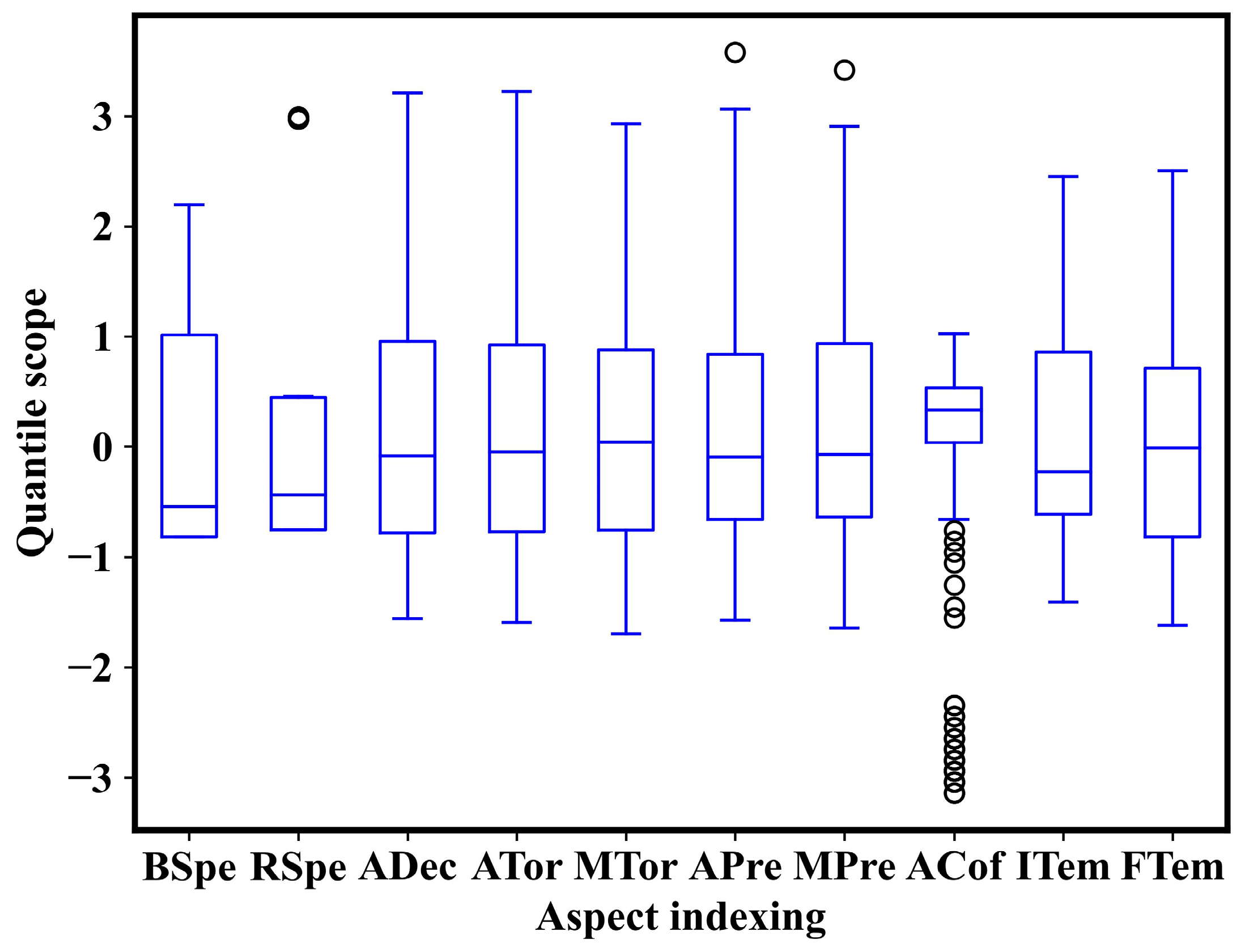
Figure 3 presents the box plot of the experimental data, where the input features of BSpe, RSpe, ADec, ATor, MTor, APre, MPre, ACof, ITem, and FTem represent the initial braking speed, release speed, average deceleration, average torque, max torque, average pressure, max pressure, average COF, initial braking temperature, and final braking temperature, respectively. The main function of the box plots is to check whether there are outliers in the data. If the data appear outside the box, it means that the data are outliers; otherwise, they are normal data.
It can be seen from Figure 3 that there are several abnormal data (circles out of the boxes in Figure 3) in the chosen features of release speed, average pressure, and max pressure, which were eliminated from the data sets because they are clearly outliers. No abnormal data were found for other features. The averaged COF data or circles out of the box were due to the various braking conditions, e.g., the various initial braking temperatures used in the dynamometer testing, and all these ACof data were used in the modeling training.

3.2. Investigating the Relationships between Features

In statistics, there are many ways to measure the degree of correlation between two variables. In this study, the correlation between the features chosen to represent the bench experimental data is evaluated by two methods, namely Pearson product moment correlation coefficient (PPMCC) method [24] and the Maximal Information Coefficient (MIC) method [25].

3.2.1. Pearson Correlation Coefficient

The Pearson product moment correlation coefficient (PPMCC) is widely used in the field of data science. PPMCC is defined as the quotient of covariance and standard deviation between two data sets, which can be calculated using Equation (3):
r = i = 1 n ( x i x ) ( y i y ) i = 1 n ( x i x ¯ ) 2 i = 1 n ( y i y ¯ ) 2
where  x ¯ , y ¯  is the average value of x and y for n experimental data, respectively. The PPMCC can range from −1 to +1, with values closer to +1 indicating a stronger positive linear correlation. Conversely, the closer the value is to −1, the stronger the negative linear correlation.
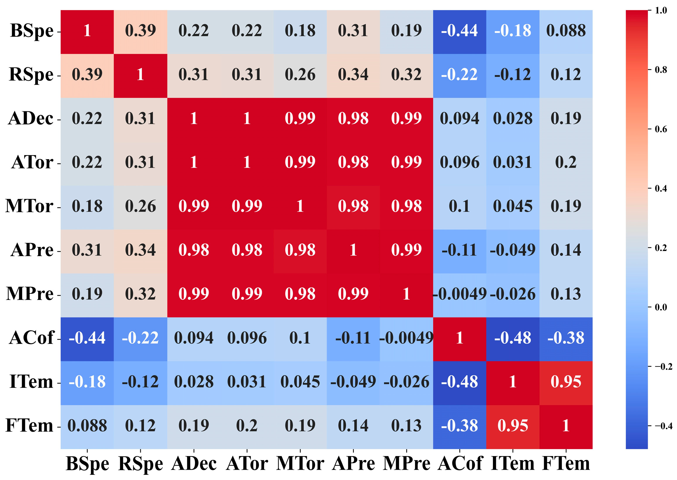
The PPMCC values between the ten input features and the output feature of ACof were calculated in turn, and the correlation values are shown in Figure 4. For example, the value of −0.48 in this figure indicates that there is a negative correlation between the initial temperature and the average COF, that is, the higher the initial temperature, the lower the average COF. This is consistent with the known inverse relationship between COF and rotor temperature.

3.2.2. Maximal Information Coefficient

The Maximal Information Coefficient (MIC) is used to measure the linear and nonlinear relationships between variables, as well as the non-functional dependence for effective measurement. Let the data set D be a finite ordered data set, which is divided into a grid G, and let  D | G  denote the probability distribution of the data set D on the grid G, then the MIC between the variables X and Y may be calculated by Equation (4):
M I C ( D ) = max x y B ( n ) I * ( D , x , y ) log 2 min { x , y }
where  I * ( D , x , y ) = max I ( D | G )  is the MIC under different grid division; i.e., for variables on the set D, the X-axis is divided into X grids, and the Y-axis is divided into Y grids of all possible grid G;  I ( D | G )  is the mutual information given the probability distribution  D | G ; B is a monotone increasing function and satisfies  B ( n ) O ( n 1 ε )  and  0 < ε < 1 . In this work,  B ( n ) = n 0.6  is chosen according to reference.
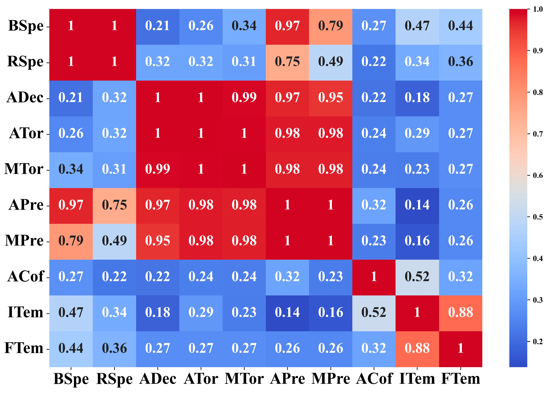
The MIC can range from 0 to 1, with larger values indicating stronger correlations. Conversely, the smaller the absolute value, the weaker the correlation. The MIC values between the ten input features and the output feature of ACof were calculated in turn, and the correlation values are shown in Figure 5. It can be seen from Figure 5 that the maximum MIC value is 0.52 between features ITem and ACof, indicating that the initial temperature of the disk is the most important factor affecting the braking COFs.

3.3. Selection of Features

Experimental data feature engineering is used to mine the bench experimental data set and investigate internal relationships between the data parameters. Here, it is used to more deeply understand the features affecting braking COFs and remove unnecessary features in order to provide concise and effective model characteristic parameters for the development of a braking COF prediction model. Based on the above PPMCC and MIC analysis results, as shown in Figure 4 and Figure 5, four input features, namely the initial braking speed (BSpe), the brake release speed (RSpe), the average hydraulic pressure (APre), and the initial rotor temperature prior to braking (ITem) were selected to be the most important in order to develop the model for predicting the output feature of the average measured COF (ACof).

4. Prediction Algorithms

The RNN (recurrent neural network) is a kind of recurrent neural network that takes sequence data as the input, re-curses all nodes (re-circulating unit) in the evolution direction of the sequence, and connects them in chains. In deep learning, the RNN is particularly suitable for processing and predicting a class of neural network models related to serial data. Figure 6 demonstrates the structure of a typical RNN cell:
The LSTM (Long Short-Term Memory) and GRU (Gate Recurrent Unit) are two good variants of RNN, which can selectively add or reduce information and can effectively alleviate the problem of RNN gradient disappearance or gradient explosion [26]. In RNN, the gradient is calculated by a multiplication of time steps, which means that the gradient is obtained by the continuous multiplication of multiple identical or similar matrices, such as the cyclic weight matrix. If the values of these matrices are less than 1, the multiplication causes the gradient to decrease exponentially, causing the gradient to disappear. The gradient explosion is similar except, if the values of the matrices are greater than 1, the gradient increases exponentially to very large values.

4.1. LSTM Method

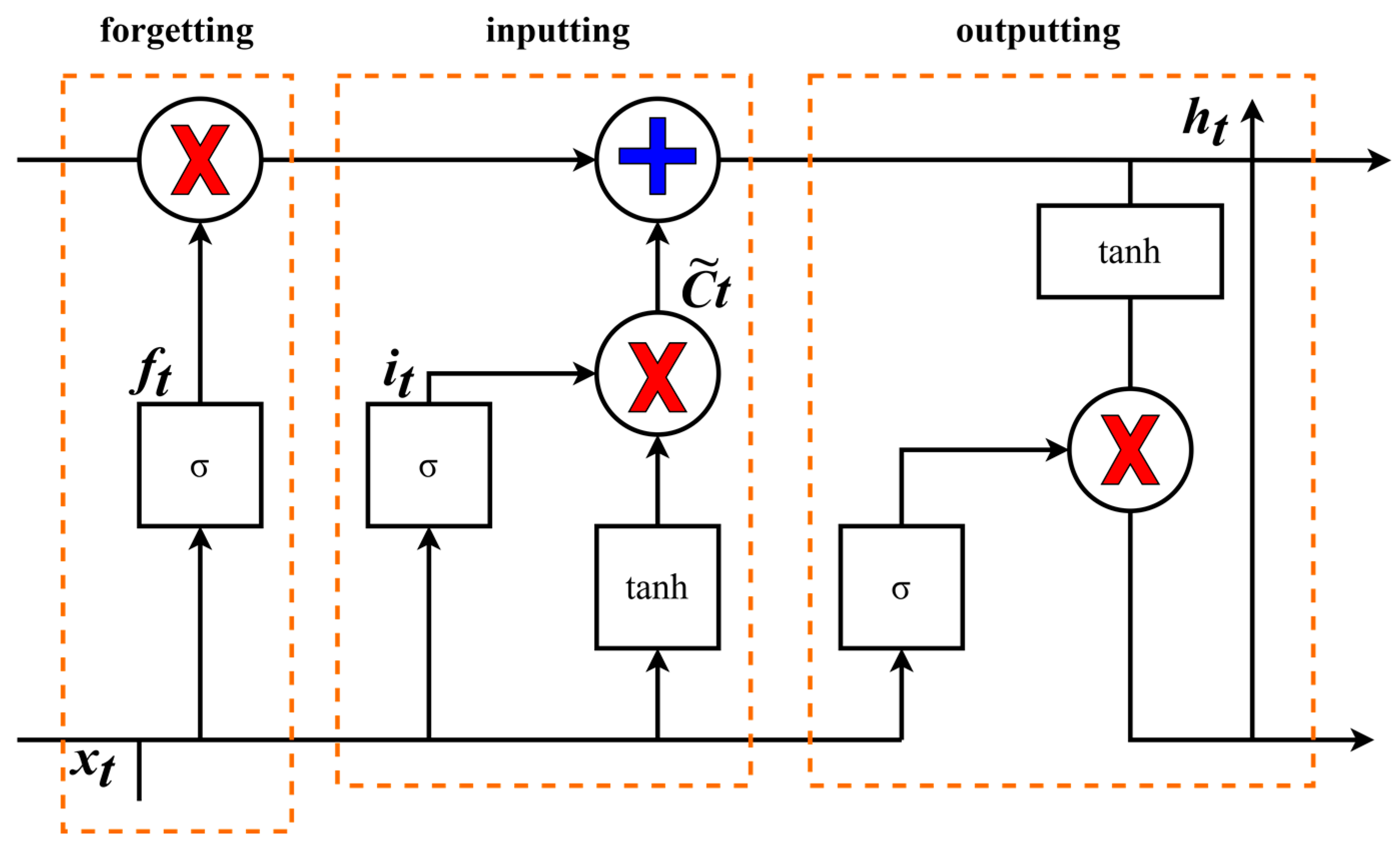
The LSTM model adds input gates, output gates, and forget gates to neurons in each layer corresponding to time points to realize the selective memory of neurons. Its structural principle is shown in Figure 7 (the red X represents multiplication and the blue + represents addition, indicating that the two functions are multiplied and added, respectively), which consists of forget gates, input gates, and output gates. The functions of these three gates are as follows:
Forget gates are used to decide what information and structure to discard from the “cell”. This layer reads the current input  x t  and the pre-neuron information  h t 1 , and it is up to  f t  to decide the discarded information.
Input gates are used to determine the new information stored in the cell state to determine the value  i t  to be updated; the tanh layer is used to create a new vector of candidate values  C ~ t  to add to the state.
Output gates are used to determine the value of the next hidden state, which contains the information of the previous input.

4.2. GRU Method

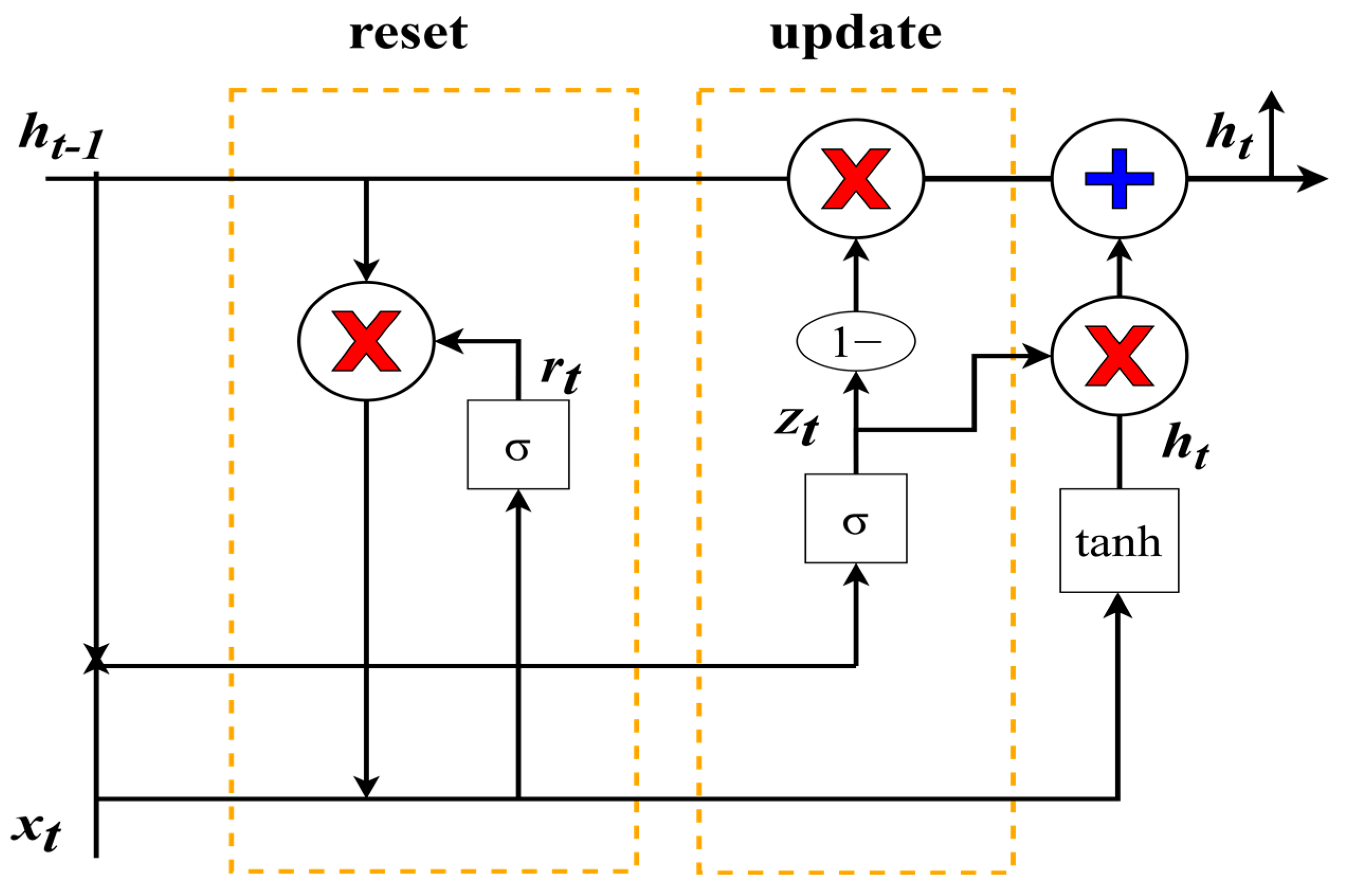
GRU is a new generation of recurrent neural networks. Similar to LSTM, GRU removes cell states and uses hidden states for information transfer. It contains only two gates: the reset gate and the update gate, which are explained as follows:
(1)
The reset gate determines how much previous information is forgotten and how new input information is combined with the previous memory, and it uses the current input information to make the hidden state forget any information that is found to be irrelevant to the prediction in the future. It also allows for the construction of more interdependent features. Essentially, the reset gate determines how much of the past data should be forgotten.
(2)
The update gate acts similarly to the forget gate and input gate in LSTM. It decides what information to forget and what new information needs to be added. Controlling how much information from previous hidden states gets passed to the current hidden state is very similar to the memory cells in LSTM networks. It helps RNNs to remember long-term information and decide whether to copy all information from the past to reduce the risk of vanishing gradients.
GRU is a very popular network because its structure is simpler and its characteristics are better than the LSTM. Therefore, this study utilizes the GRU algorithm to predict braking COFs.

Gated Computation for GRU

The structure of a GRU neural network is shown in Figure 8, where the red X represents multiplication and the blue + represents addition, indicating that the two functions are multiplied and added, respectively. Compared with the traditional recurrent neural networks, the advantage of the GRU neural network is that it only contains two gates, namely the reset gate and update gate, and the detailed operation of both of which are described below.
(1)
Update gate.
At time step t, we first need to compute the update gate  Z t  using the following formula:
Z t = σ ( ω Z [ h t , x t ] )
where  x t  is the input vector at the t-th time step, that is, the t-th component of the input sequence x, which undergoes a linear transformation when multiplied by the weight matrix  ω Z . The  h t  vector holds the information from the previous time step t, which also undergoes the linear transformation. The update gate adds these two pieces of information and feeds them into the Sigmoid activation function, thus compressing the activation result to be between 0 and 1.
(2)
Reset gate.
Essentially, the reset gate determines how much of the past information needs to be forgotten, which can be calculated using the following expression:
r t = σ ( ω Z [ h t 1 , x t ] )
This expression is the same as the expression for the update gate, but the parameters of the linear transformation and its use are different. The  h t 1  holds the information from the previous time step t − 1, which also undergoes the linear transformation.
(3)
Current memory content.
Now let us discuss in detail how exactly these gates affect the final output. In the use of reset gates, the new memory content will use the reset gate to store relevant information from the past to calculate the new data:
h t = tanh ( ω [ r t × h t 1 , x t ] )
The input  x t  and the previous time information are first subjected to a linear transformation by the right multiplication matrix  w . Then, the Hadamard product of the reset gate  r t  with  h t 1    is computed. Because the reset gate computed earlier is a vector of 0 to 1 values, it will measure the magnitude of the gate opening. For example, if the gating value for an element is 0, it means that the information for that element has been completely forgotten. The Hadamard product will determine the previous information to retain and forget. The results of these two calculations are added together and then put into the hyperbolic tangent activation function.
(4)
The final memory of the current time step.
In the final step, the network needs to compute the  h t  vector, retain the information from the current cell and pass it on to the next cell. In this process, it needs to use the update gate, which determines what information needs to be collected in the current memory content  h t  and the previous time step  h t 1 . This process can be expressed as:
h t = ( 1 z t ) × h t 1 + z t × h t ˜
where  z t  is the activation result of the update gate, which also controls the inflow of information in the form of gate control. The Hadamard product of  z t  and  h t 1  represents the information retained in the final memory at the previous time, which, together with the information retained by the current memory in the final memory, equals the output of the final gated loop unit.

4.3. Model Evaluation Index

4.3.1. Correlation Index R2

R 2  is the determining coefficient, also known as the correlation index, which represents the degree of fit of the regression equation to the data set as a means of measuring the reliability of the prediction of the regression equation. The closer the value is to 1, the closer the actual prediction point is to the goal line, the better the degree of fit of the model to the data, and therefore, the more accurate the prediction of the model. Equation (9) can be used to calculate the  R 2  value ranges from 0 to 1:
R 2 = 1 R S S T S S = 1 i = 1 n ( y i y i ^ ) 2 i = 1 n ( y i y i ¯ ) 2
where RSS is the sum of residual squares, namely:
R S S = i = 1 n ( y i y i ^ ) 2
And TSS is the sum of the squares of the total deviation, i.e.:
T S S = i = 1 n ( y i y i ¯ ) 2

4.3.2. MAE Index

The mean absolute error (MAE), also known as mean absolute deviation, measures the absolute difference between the real value and the predicted value. The smaller it is, the more accurate the prediction is. MAE is the deviation between all the observed values and the arithmetic mean value, which is obtained by averaging the absolute values. The calculation formula is as follows:
M A E = 1 n i = 1 n h ( x i ) y i
where  h ( x i )  is the predicted value and  y i  is the measured value.
The MAE avoids the positive and negative errors canceling each other, so it can more accurately reflect the magnitude of the prediction error than the correlation index.

5. Prediction Results

5.1. Model Comparison

The train_test_split function of the sklearn routine within the Python library is used to split the whole dataset into a training set, a validation set, and a test set, accounting for 60%, 20%, and 20% of the available dynamometer data, respectively. The training set is used for model training, the validation set is used for preliminary evaluation of whether the model training results meet the requirements, and the test set is used for model prediction. The final evaluation index of the model was evaluated by comparing the final prediction results with the values of the test set. Then, the pytorch, numpy, and other routines within the Python library are used to define the LSTM and GRU algorithm models, respectively. The model is trained by inputting data representing the independent input features and target output features from the training data set. Predictions are then made using the validation data set composed of a new set of test variables in order to evaluate the model performance and adjust the hyperparameters. The test set data is retained as unique data for the final evaluation of the optimized model performance.
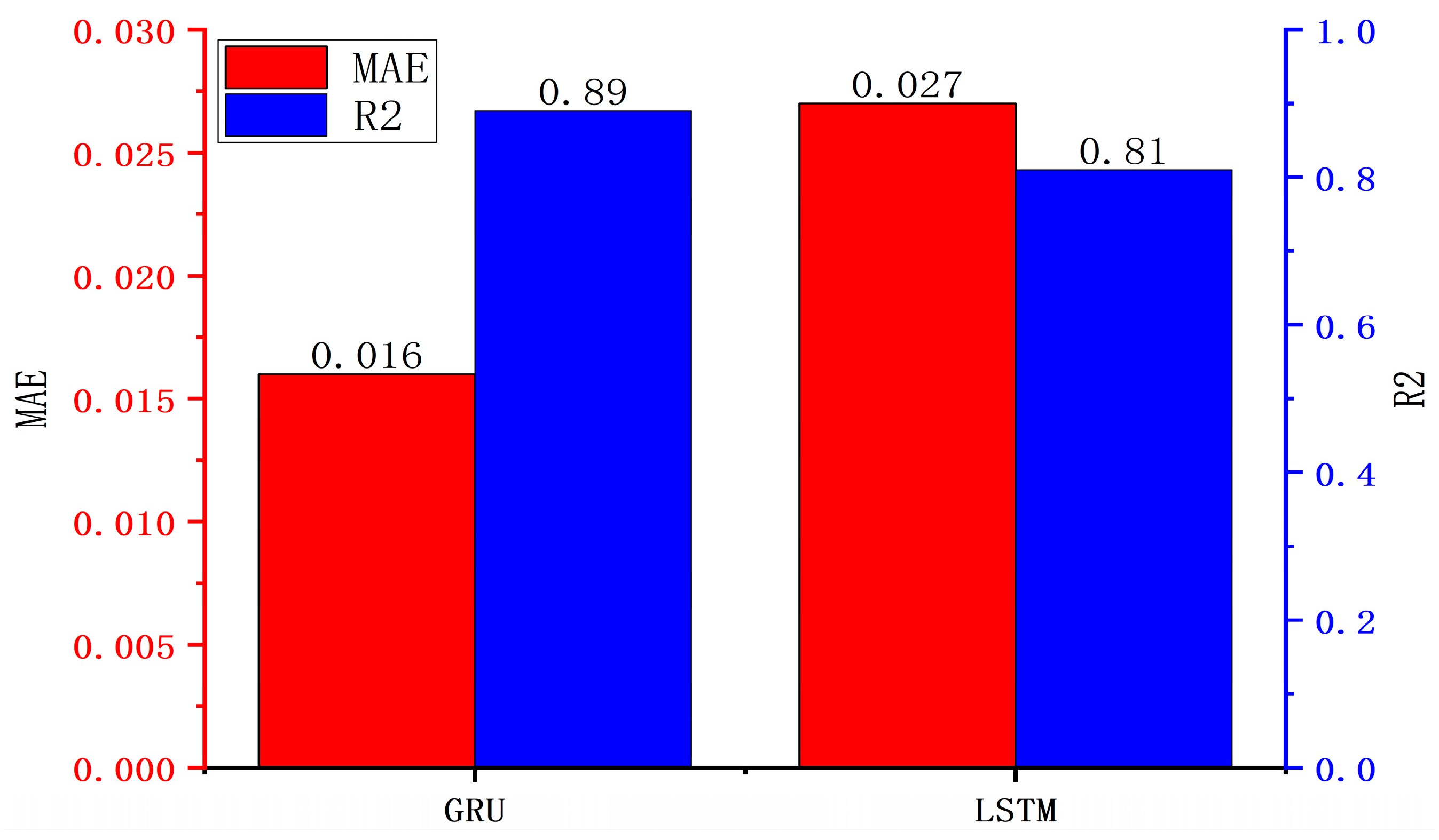
Figure 9 represents the MAE and the R2 evaluations for the GRU and LSTM predictions for the validation data set, respectively. It is observed from Figure 9 that the MAE of GRU is smaller, while the R2 value of GRU is larger. The closer the MAE is to 0 and the closer the R2 value is to 1, the more accurate the prediction. Therefore, the GRU model was selected in preference to the LSTM to further develop the prediction model for the braking COF.

5.2. Predictions of the GRU Model

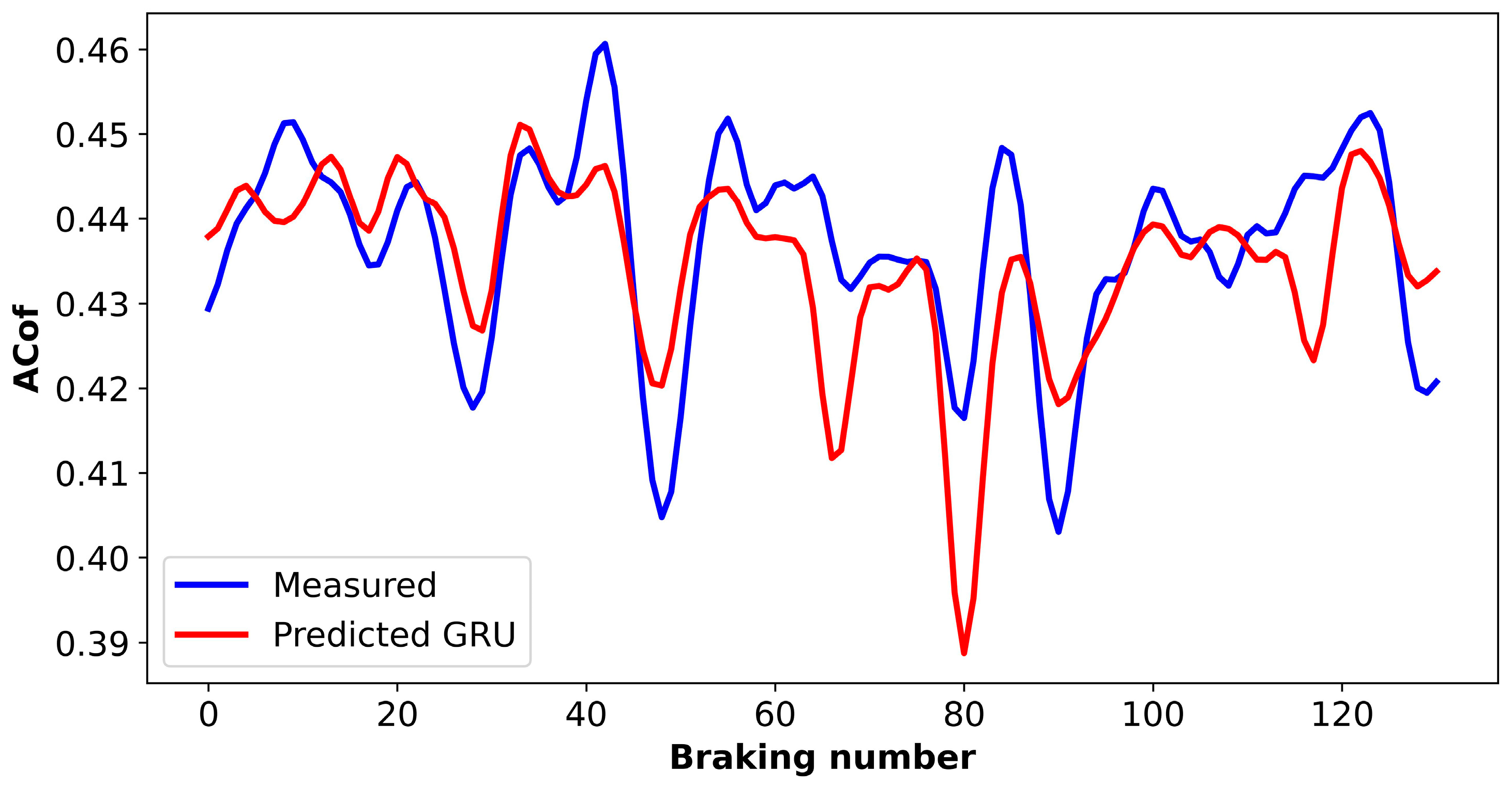
Table 2 shows the names and default values of the parameters required for the GRU model. The number of input features has already been set to 4 (BSpe, RSpe, APre, ITem), and the number of output features is 1 (ACof). Based on these parameters, the COF predicted by the GRU algorithm are compared with the validation set of measured data from the bench tests, as shown in Figure 10. It can be seen that, although the general trend of the measured data is well predicted, there are some large discrepancies approaching a maximum of 10% between the predicted and measured COF values. Hence, it was decided to implement the PSO method in order to further optimize the GRU algorithm.

5.3. Predictions of the GRU Model Optimized with the PSO Algorithm

The particle swarm optimization (PSO) algorithm is a global optimization algorithm based on the bionic study of bird foraging behavior in nature. It considers each possible solution in the global variable as a particle that has its own direction and speed so that all particles move towards the local optimal position. By constantly updating the local optimal position  x b e s t  and the global optimal position  P b e s t  of the particle, an optimal solution of the objective function can be obtained.
The hyperparameters of the GRU neural network are classified as the attributes of the particle, and the fitness of the particle is evaluated. Through continuous iteration, the optimal particle is updated. Finally, the optimal particle with the best fitness is obtained to give the required optimal hyperparameters. Figure 11 illustrates the optimization process for the braking COF prediction model using the combined PSO–GRU algorithm.
In summary, the PSO is used to optimize the hyperparameters of the GRU algorithm to find the best hyperparameters, and the best hyperparameters are then employed in the GRU algorithm to predict the braking COFs. If the acceptance criterion of R2 > 0.9 is not achieved in the predicted values, the PSO optimization is repeated and the GRU algorithm rerun until the required level of accuracy has been achieved.
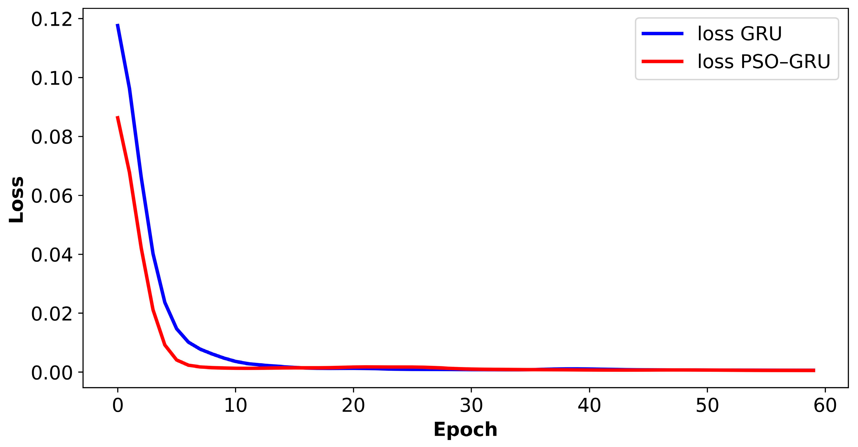
The value of the loss function (loss) is a measure of the discrepancy between the predicted value and the measured value. Figure 12 shows that the loss curve of the PSO–GRU model converges faster to a zero value than that of the GRU model used in isolation.
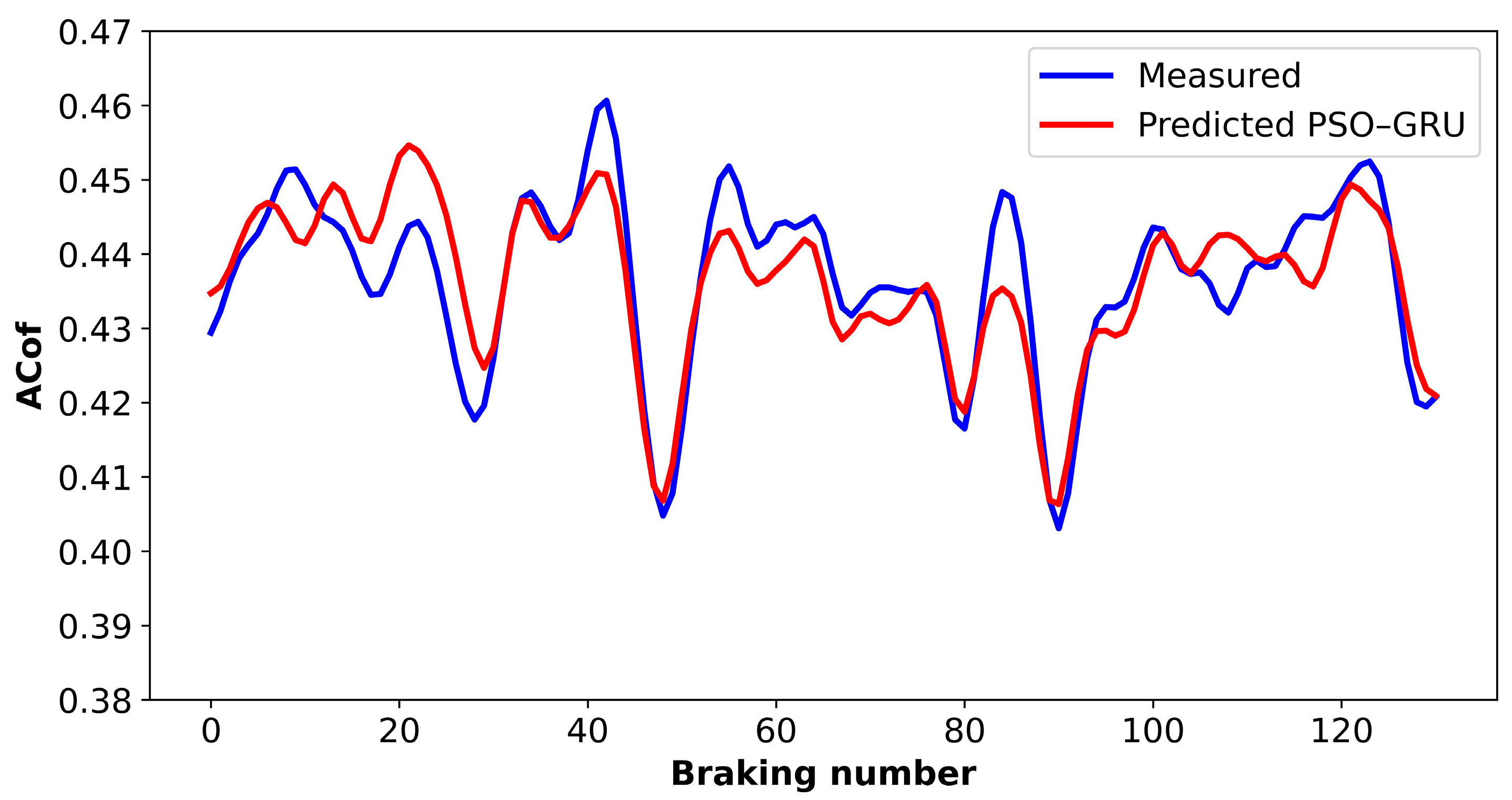
Figure 13 presents the measured COFs and the predicted results from the combined PSO–GRU model for the validation data set. It is obvious from the comparison of Figure 10 and Figure 13 that the PSO–GRU algorithm exhibits superior prediction performance compared to the GRU-only algorithm.

5.4. Model Comparison

The same experimental data were input into the GRU algorithm and PSO–GRU algorithm, and the model evaluation indicators (R2, MAE, training time) obtained from the GRU algorithm for the validation data set are compared with those from the combined PSO–GRU algorithm in Table 3. Compared with the GRU algorithm before optimization, the R2 of the combined PSO–GRU algorithm is increased by 4.7%, the MAE is reduced by 14.3%, and the prediction speed is increased by 40.1%.

6. Conclusions

The rapid and effective prediction of COFs is of great significance for the study of braking performance and frictional noise, and also to further understand the factors controlling friction. One of the biggest challenges to this goal is the nonlinearity of the COF, which is affected by a large number of factors.
In this study, a GRU neural network combined with an improved PSO algorithm has been successfully used to solve the complex nonlinear problem of predicting braking COFs from a limited set of experimental data. The PSO algorithm has been used to improve the convergence rate and prediction accuracy of the original GRU neural network. The PSO–GRU algorithm increased the R2 of the prediction by 4.7%, reduced the MAE by 14.3%, and increased the prediction speed by 40.1%. It is clear from the results that, after applying the PSO parameter optimization algorithm, the GRU prediction model has a shorter training time and better prediction accuracy for an unseen test data set than the standalone GRU model. Therefore, the combined PSO–GRU algorithm is a better choice for the accurate prediction of COFs from a limited set of experimental data.
The prediction of braking COFs with the PSO–GRU algorithm has significance not only for the fast development and evaluation of an automotive braking system, but also provides meaningful reference for solving complicated tribological problems in other applications.

Author Contributions

Conceptualization, S.W.; Methodology, S.W.; Validation, S.W. and Y.Y.; Formal analysis, Y.Y. and S.W.; Investigation, Y.Y. and S.L.; Data curation, S.W. and Y.Y.; Writing—original draft preparation, Y.Y.; Writing—review and editing, S.W. and D.B.; Supervision, S.W. All authors have read and agreed to the published version of the manuscript.

Funding

This research was financially supported by the Science and Technology Committee of Shanghai Municipality (Grant No. 18060502400) and Natural Science Foundation of Shanghai (Grant No. 21ZR1445000).

Data Availability Statement

The data presented in this study are available upon request from the corresponding author.

Conflicts of Interest

The authors declare no conflicts of interest.

Nomenclature

SymbolDefinitionUnit
ACofaverage COF/
ADecaverage decelerationg
APreaverage pressurebar
AToraverage torqueNm
Bmonotone increasing function/
BSpeinitial braking speedkph
COFcoefficient of friction/
COFscoefficients of friction/
FTemfinal braking temperature°C
GRUgated recurrent unit/
hthidden state at time step t/
h(xi)predicted value/
I(D|G)probability distribution/
I*(D, x, y)probability distribution under different grid division
ITeminitial braking temperature°C
LSTMlong short-term memory/
MAEmean absolute error/
MICmaximal information coefficient/
MIC(D)value of MIC/
MPremax pressurebar
MTormax torqueNm
PPMCCPearson product moment correlation coefficient/
PSOparticle swarm optimization/
rvalue of PPMCC/
rtactivation vector of reset gate/
R2evaluation of the model/
RSperelease speedkph
RSSthe sum of residual squares/
TSSthe sum of the squares of the total deviation/
vparticleparticle velocity/
x max maximum value of all samples/
x min minimum value of all samples/
ximeasured value of x/
x normalized result/
x ¯ average value of x/
X standardized value/
y ¯ average value of y/
yimeasured value of y/
Ztactivation vector of update gate/
μ mean of all samples/
σ standard deviation of all samples/
ω z weight matrix of the update gate/
ω r weight matrix of the reset gate/

References

  1. Zhu, D.; Yu, X.; Sai, Q.; Wang, S.; Barton, D.; Fieldhouse, J.; Kosarieh, S. Noise and vibration performance of automotive disk brakes with laser-machined M-shaped grooves. Proc. Inst. Mech. Eng. Part D J. Automob. Eng. 2022, 237, 978–990. [Google Scholar] [CrossRef]
  2. Wang, S.; Guo, W.; Zeng, K.; Zhang, X. Characterization of automotive brake discs with laser-machined surfaces. Automot. Innov. 2019, 2, 190–200. [Google Scholar] [CrossRef]
  3. Khairnar, H.P.; Phalle, V.M.; Mantha, S.S. Estimation of automotive brake drum-shoe interface friction coefficient under varying conditions of longitudinal forces using Simulink. Friction 2015, 3, 214–227. [Google Scholar] [CrossRef]
  4. Riva, G.; Varriale, F.; Wahlström, J. A finite element analysis (FEA) approach to simulate the coefficient of friction of a brake system starting from material friction characterization. Friction 2021, 9, 191–200. [Google Scholar] [CrossRef]
  5. Meng, Y.; Xu, J.; Ma, L.; Jin, Z.; Prakash, B.; Ma, T.; Wang, W. A review of advances in tribology in 2020–2021. Friction 2022, 10, 1443–1595. [Google Scholar]
  6. Balaji, V.; Lenin, N.; Anand, P.; Rajesh, D.; Raja, V.B.; Palanikumar, K. Brake squeal analysis of disc brake. Mater. Today Proc. 2021, 46, 3824–3827. [Google Scholar] [CrossRef]
  7. Crolla, D.A.; Lang, A.M. Brake noise and vibration: The state of the art. Veh. Tribol. 1991, 18, 165–174. [Google Scholar]
  8. Oberst, S.; Lai, J. Chaos in brake squeal noise. J. Sound Vib. 2011, 330, 955–975. [Google Scholar] [CrossRef]
  9. Jarvis, R.P.; Member, B.M. Vibrations induced by dry friction. Proc. Inst. Mech. Eng. 1963, 178, 847–857. [Google Scholar] [CrossRef]
  10. Nishiwaki, M. Generalized theory of brake noise. Proc. Inst. Mech. Eng. Part D J. Automob. Eng. 1993, 207, 195–202. [Google Scholar] [CrossRef]
  11. Zhang, W.; Guo, W.; Liu, X.; Liu, Y.; Zhou, J.; Li, B.; Lu, Q.; Yang, S. LSTM-based analysis of industrial IoT equipment. IEEE Access 2018, 6, 23551–23560. [Google Scholar] [CrossRef]
  12. Jiang, W.; Zhang, N.; Xue, X.; Xu, Y.; Zhou, J.; Wang, X. Intelligent deep learning method for forecasting the health evolution trend of aero-engine with dispersion entropy-based multi-scale series aggregation and LSTM neural network. IEEE Access 2020, 8, 34350–34361. [Google Scholar] [CrossRef]
  13. Zhang, X.; Zhang, M.; Xiang, Z.; Mo, J. Research on diagnosis algorithm of mechanical equipment brake friction fault based on MCNN-SVM. Measurement 2021, 186, 110065. [Google Scholar] [CrossRef]
  14. Zhang, M.; Zhang, X.; Mo, J.; Xiang, Z.; Zheng, P. Brake uneven wear of high-speed train intelligent monitoring using an ensemble model based on multi-sensor feature fusion and deep learning. Eng. Fail. Anal. 2022, 137, 106219. [Google Scholar] [CrossRef]
  15. Yang, X.; Chen, L. Dynamic state estimation for the advanced brake system of electric vehicles by using deep recurrent neural networks. IEEE Trans. Ind. Electron. 2019, 99, 9536–9547. [Google Scholar]
  16. Šabanovič, E.; Žuraulis, V.; Prentkovskis, O.; Skrickij, V. Identification of road-surface type using deep neural networks for friction coefficient estimation. Sensors 2020, 20, 612. [Google Scholar] [CrossRef] [PubMed]
  17. Stender, M.; Tiedemann, M.; Spieler, D.; Schoepflin, D.; Hoffmann, N.; Oberst, S. Deep learning for brake squeal: Brake noise detection, characterization and prediction. Mech. Syst. Signal Process. 2021, 149, 107181. [Google Scholar] [CrossRef]
  18. Wang, S.; Zhong, L.; Niu, Y.; Liu, S.; Wang, S.; Li, K.; Wang, L.; Barton, D. Prediction of frictional braking noise based on brake dynamometer test and artificial intelligent algorithms. Proc. Inst. Mech. Eng. Part D J. Automob. Eng. 2021, 236, 2681–2695. [Google Scholar] [CrossRef]
  19. Alexsendric, D.; Barton, D.C. Neural network prediction of disc brake performance. Tribol. Int. 2009, 42, 1074–1080. [Google Scholar] [CrossRef]
  20. Alexsendric, D.; Barton, D.C.; Vasic, B. Prediction of brake friction materials recovery performance using artificial neural networks. Tribol. Int. 2010, 43, 2092–2099. [Google Scholar] [CrossRef]
  21. J2521_201304; Disc and Drum Brake Dynamometer Squeal Noise Test Procedure. SAE International: Warrendale, PA, USA, 2013.
  22. Shalabi, L.A.; Shaaban, Z.; Kasasbeh, B. Data mining: A preprocessing engine. J. Comput. Sci. 2006, 2, 735–739. [Google Scholar] [CrossRef]
  23. Curtis, A.E.; Smith, T.A.; Ziganshin, B.A.; Elefteriades, J.A. The mystery of the Z-score. Aorta 2016, 4, 124–130. [Google Scholar] [CrossRef] [PubMed]
  24. Benesty, J.; Chen, J.D.; Huang, Y. On the importance of the Pearson correlation coefficient in noise reduction. IEEE Trans. Audio Speech Lang. Process. 2008, 16, 757–765. [Google Scholar] [CrossRef]
  25. Reshef, D.N.; Reshef, Y.A.; Finucane, H.K.; Grossman, S.R.; McVean, G.; Turnbaugh, P.J.; Lander, E.S.; Mitzenmacher, M.; Sabeti, P.C. Detecting novel associations in large data sets. Science 2011, 334, 1518–1524. [Google Scholar] [CrossRef]
  26. Zargar, S. Introduction to Sequence Learning Models: RNN, LSTM, GRU; Department of Mechanical and Aerospace Engineering: Colorado Springs, CO, USA, 2021. [Google Scholar]
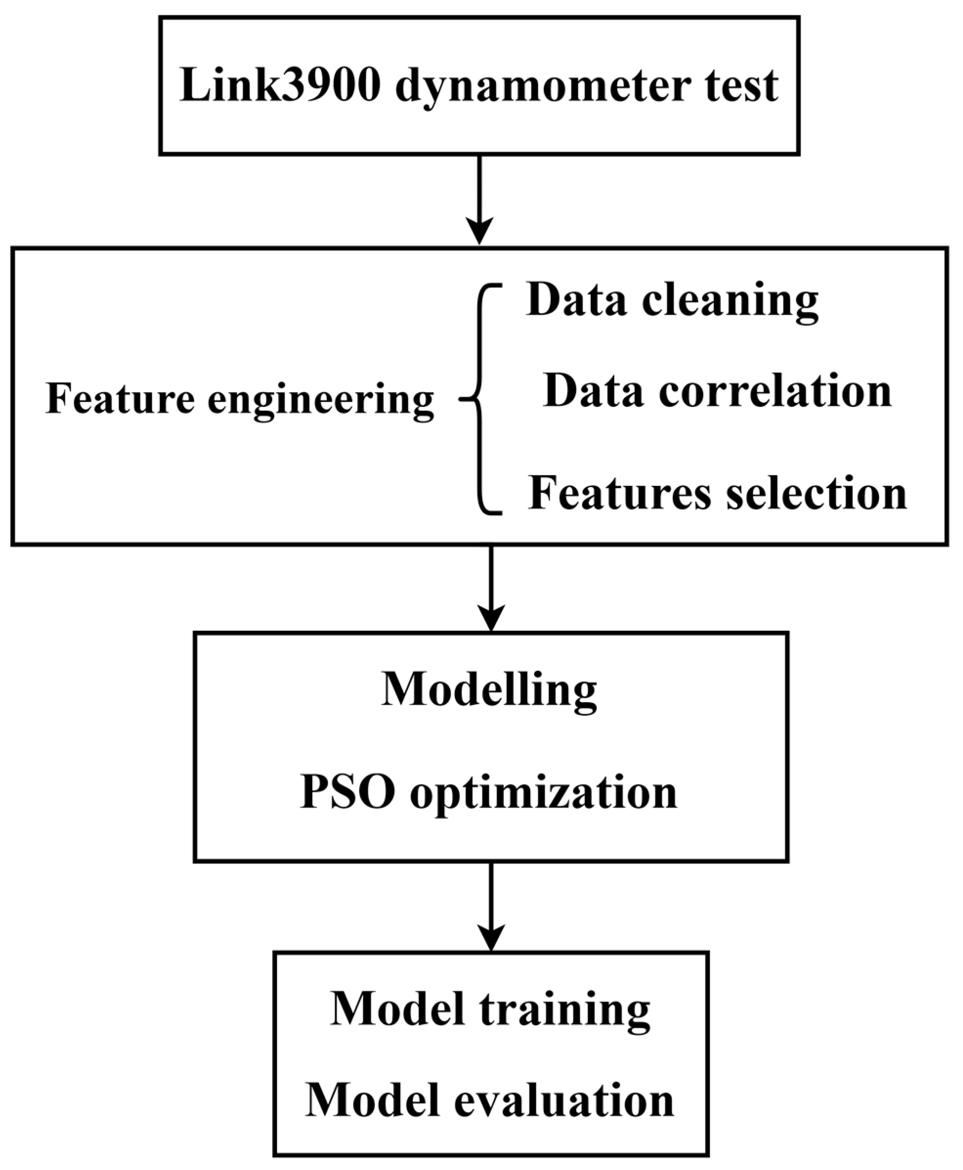
Figure 1. Research procedure and the structure of the paper.
Lubricants 12 00195 g001
Figure 2. LINK3900 brake performance test rig (partial).
Lubricants 12 00195 g002
Figure 3. BP box plot.
Lubricants 12 00195 g003
Figure 4. PPMCC matrix heatmap.
Lubricants 12 00195 g004
Figure 5. MIC matrix heatmap.
Lubricants 12 00195 g005
Figure 6. RNN cell expansion structure diagram.
Lubricants 12 00195 g006
Figure 7. Gated structure in LSTM.
Lubricants 12 00195 g007
Figure 8. Gated structure in GRU.
Lubricants 12 00195 g008
Figure 9. Evaluation metrics.
Lubricants 12 00195 g009
Figure 10. Comparison of predicted and measured COF for test set.
Lubricants 12 00195 g010
Figure 11. Flow chart of PSO–GRU prediction model for brake COF.
Lubricants 12 00195 g011
Figure 12. Loss curves of GRU model and PSO–GRU model for test set.
Lubricants 12 00195 g012
Figure 13. Comparison of the predicted and measured COF for test set after model optimization.
Lubricants 12 00195 g013
Table 1. Screenshot of typical experimental data obtained from braking tests.
StopBrake Speed (kph)Release Speed (kph)Stop Time (s)Avg Decel (g)Avg Torq (Nm)Max Torq (Nm)Avg Press (bar)Max Press (bar)Avg μ LevelInitial Temp Rotor CFinal Temp Rotor CPeak Level (dBA)Frequency of Peak (Hz)Above Threshold 70 dBA
179.730.08.3770.1856561715.015.80.4410015873.52800YES
280.030.04.680.351087114529.930.60.4210016369.95900
380.130.08.320.1856962015.015.70.4410015859.25950
479.830.07.010.2267473018.018.60.4410015769.05975
580.030.05.990.2681987721.922.50.4310015870.92800YES
679.830.03.830.441357140437.838.60.4210016471.52800YES
779.730.08.350.1856361515.015.90.4410015669.16200
879.730.05.250.31948101025.926.50.4310016069.95975
980.130.07.060.2267072618.018.50.4310015767.66325
1080.030.04.190.401232128833.934.60.4210016071.42925YES
1180.030.08.360.1856462115.015.80.4410015568.66350
Table 2. Description of the parameters required by the GRU.
ParameterParameter InterpretationDefault
input_sizeNumber of input features4
output_sizeNumber of output features1
rnn_unitHidden layers64
lrLearning rate0.001
epochIterations100
Table 3. Performance comparison of GRU and LSTM algorithms.
ModelR2MAETraining Time (ms)
GRU0.8930.016220
PSO–GRU0.9350.014157
Disclaimer/Publisher’s Note: The statements, opinions and data contained in all publications are solely those of the individual author(s) and contributor(s) and not of MDPI and/or the editor(s). MDPI and/or the editor(s) disclaim responsibility for any injury to people or property resulting from any ideas, methods, instructions or products referred to in the content.