Machine Learning-Based Predictions of Metal and Non-Metal Elements in Engine Oil Using Electrical Properties

Abstract

This study investigates the influence of six metallic and non-metallic elements (Fe, Cr, Pb, Cu, Al, Si) on the quality of engine oil under normal, cautious, and critical conditions. To achieve this, the research employs the Design of Experiments (DoE) approach, specifically the Box–Behnken Design (BBD) method, for designing experiments. The electrical properties of 70 engine oil samples prepared under varying conditions were analyzed. Machine learning models, including RBF, ANFIS, MLP, GPR, and SVM, were utilized to predict the concentrations of the six pollutants in the lubricant oil samples based on their electrical characteristics. The models’ performance was assessed using RMSE and R² indicators during train, test, and All stages. The results revealed that the Radial Basis Function (RBF) model exhibited the best overall performance (RMSE = 0.01, R² = 0.99). The study proceeds with optimizing RBF model parameters, such as hidden size (best = 17), spread (best = 0.4 or higher), and training algorithm (best = trainlm), to estimate each pollutant individually. The generalizability of the model was assessed by reducing the training data percentage and increasing the testing data percentage. The results demonstrated the model’s proper performance for all pollutants in various training sizes (RMSE = 0.01, R² = 0.99). However, as the training data ratio reduced to 60:40 and 50:50, the model’s performance in estimating Cu deteriorated, resulting in increased RMSE values (10.76 or 11.85) and decreased R² values (0.89 or 0.87) across the All step. This academic research hopes to contribute to the field of applied studies, considering the inherent complexities of lubricants and the challenges in measuring small-scale electrical properties.

1. Introduction

An engine’s durability is crucial throughout a car’s lifespan as it significantly impacts the performance and safety of a vehicle [1,2]. A range of techniques has been developed for forecasting engine component lifespan and evaluating durability [3,4,5,6]. These methodologies involve a combination of analytical, experimental, and computational approaches that enable engineers to predict the performance and reliability of engine components over their intended service life. These techniques consider various factors such as material properties, operating conditions, and environmental stresses to provide insights into component wear, fatigue, and failure mechanisms [7,8]. By utilizing these methodologies, engineers can optimize component designs, improve manufacturing processes, and minimize maintenance costs while ensuring safe and reliable engine operation.

To prevent engine problems in a car and ensure its smooth operation, several methods can be followed. These encompass regular maintenance, in step with the producer’s suggestions, monitoring engine diagnostics, addressing common problems right away, retaining the right fluid ranges, using the right fuel and lubricants, and using responsibly [9,10]. The lubrication of an engine is vital for its functioning as it facilitates reduced friction, dissipates heat, and prevents wear and corrosion of the engine’s moving elements [11,12]. The effectiveness of the lubrication device is directly associated with the engine’s reliability and efficiency [13]. Regular attention to the engine’s lubrication system is necessary to ensure its reliability and performance. Lubrication plays a critical role in the engine running easily by minimizing friction among shifting elements, reducing heat generation, and forestalling put and tear [14,15]. Effective maintenance programs, including preventative maintenance and diagnostic equipment, are important for fee-effective transit service [16,17]. Studies have demonstrated that dynamic probabilistic models, risk-based approaches, and condition monitoring techniques can be employed to forecast the likelihood of main engine lubrication failure and make informed decisions regarding maintenance and repairs [18]. A range of factors, including the age of the engine, working conditions, maintenance history, and lubricant quality, can impact the possibility of lubrication failure [19,20]. Further studies have been conducted to analyze the accumulation of mechanical combos, such as wear debris and contaminants, within the engine lubrication device and how oil degradation affects the system’s overall performance. This accumulation of mechanical combos can lead to friction, and corrosion, which could bring about reduced engine efficiency and extended preservation costs [21]. Oil degradation, because of factors that include excessive temperatures, oxidation, and nitration, also can negatively affect the lubrication system’s overall performance by altering the lubricant’s viscosity, lowering its ability to protect the engine’s components, and increasing the chance of lubricant failure [22]. In fact, oil quality refers to the effectiveness and performance characteristics of the engine oil in terms of its ability to lubricate, cool, and protect engine components. Oil quality can degrade due to factors like oxidation, which affects its lubrication and cooling functions. Even if the viscosity remains acceptable, the accumulation of metal particles from wear can exceed permissible levels, indicating compromised oil quality (a sign of failure and wear of engine parts). This research seeks to identify the presence of both metallic and non-metallic elements (Fe, Cr, Pb, Cu, Al, Si) in engine oil by assessing its electrical properties, which could provide insights into the overall quality of the oil. Furthermore, the development of data prediction models for lubrication systems can aid in monitoring and maintaining their performance parameters [23]. Recent advancements in machine learning, particularly artificial neural networks, have significantly improved the prediction of lubricant performance parameters, such as friction, wear, and lubrication film thickness [24]. These advancements have also led to the development of online lubrication oil condition monitoring and remaining useful life prediction techniques, which utilize commercially available online sensors and particle filtering [25,26]. Furthermore, the application of artificial neural networks has shown promise in accurately recognizing changes in the lubrication system, such as the appearance of air bubbles in the lubricant [27].

The electrical properties of materials play a crucial role in condition monitoring as they can predict the behavior of structures and materials under various conditions. For instance, the dissipation factor and loss index can indicate the health of insulating materials, with changes in these properties signaling the need for material replacement [28]. By monitoring the electrical impedance of piezoelectric structures, researchers can determine mechanical boundary conditions and predict their behavior [29]. Impedance-based health monitoring, using techniques such as the electromechanical impedance method, can also provide valuable information about the state of a structure [30]. The electrical properties of thermal oxide on 3C-SiC layers can help assess the state of insulation systems in high-voltage equipment [31]. Environmental conditions and material composition can significantly influence the electrical properties of textiles, further highlighting the importance of these properties in condition monitoring [32]. Smart composite hydrogels are used for wearable disease monitoring, and their electrical properties can detect changes in the body [33]. Electrical insulation monitoring involves diagnosing parameters such as loading, temperature, gas analysis, partial discharge activity, and bushing condition to assess the state of insulation systems [34]. By understanding and modeling these properties, researchers and engineers can develop more effective and reliable monitoring systems for various industries and applications.

A range of studies have explored the use of electrical properties for monitoring engine oil condition. Engine oil conditions can be monitored using electrical properties such as dielectric and magnetic characteristics. The advantages of using electrical properties to monitor engine oil conditions include the ability to provide information about the oil’s condition and the probable time for its change, as well as the potential to develop online condition monitoring devices for engine oil [35,36]. Research has shown that the dielectric properties of lubricating oil are reasonably well correlated with viscosity, making it a potential basis for oil condition monitoring systems [37]. Additionally, a study has been conducted to assess the relationship between the engine oil deterioration condition and the electrical property of the dielectric constant, which is related to physical properties such as total acid number (TAN), total base number (TBN), and viscosity [36]. These findings suggest that electrical properties can be used to develop online condition monitoring devices for engine oil, providing information about its condition and the probable time for its change [38,39]. The metal and non-metal content of lubricating oil can be analyzed to determine the condition of engine components and the wear caused by friction or pollution [40,41]. Wu et al. demonstrated the differentiation of nonferrous metal particles in lubrication oil using an inductive sensor [42]. Dielectric spectroscopy has been successfully used to monitor the degradation of engine lubricating oil, with the potential to determine properties such as oxidation duration, total acid number, and insoluble content [43]. It has also been employed in classifying engine lubricating oils based on SAE grade and source, demonstrating its ability to provide compositional and structural information [44]. While these studies do not directly address the determination of content in lubricants by dielectric spectroscopy, they do suggest its potential for such applications. However,

Table 1. A summary of studies focused on measuring the electrical properties of motor lubricants.

Goal	Measured Parameter	Electrical Settings	Description	Ref.
Soot and diesel measurements	Impedance	20 Hz–600 KHz	Electrochemical Impedance Spectroscopy (EIS)	[46]
Oxidation Duration (OD), Total Acid Number (TAN), and Insoluble Content (IC)	Dielectric	50 KHz–16 MHz	Dielectric Spectroscopy (DS) compared with Fourier Transform Infrared Spectroscopy (FTIR)	[43]
Iron Content	Impedance	40 Hz–10 KHz	liquid test fixture 16452	[47]
Moisture Content	Impedance	100 Hz–100 KHz	liquid test fixture 16452	[48]
focused on the change in the dielectric at different temperatures with two different gaps between electrodes	Dielectric	0.001 Hz–100 Hz	Dielectric Spectroscopy (DS)	[49]
Diagnosis of the State	Impedance	200 Hz–2 MHz	-	[50]
Diagnosis of the State	Impedance	0.1 Hz–10 KHz	Electrochemical Impedance Spectroscopy (EIS), constituted the input feature matrix for the classifiers. Classifiers, based on Support Vector Machine (SVM) and Artificial Neural Network applied separately.	[51]
Moisture measurement	electrochemical impedance spectroscopy (EIS) and dielectric constant calculation based on the measured impedance values.	0.01 Hz–100 Hz	-	[52]
Dielectric (ε′, ε″, tan δ)	The metal and non-metal content Fe, Pb, Cu, Cr, Al, Si, Zn	2.4 GHz, 5.8 GHz, 7.4 GHz, 9.6 GHz	The ANN method is used for monitoring the correlation between predicted and observed dielectric characteristics.	[53]
The metal and non-metal content Fe, Pb, Cu, Cr, Al, Si, Zn	Dielectric (ε′, ε″, tan δ)	2.4 GHz, 5.8 GHz, 7.4 GHz	The soft computing models are used to predict the elemental spectroscopy of lubricants through their electrical properties.	[54]

provides a summary of the literature. Some literature studies the feasibility of measuring the features of used lubricants exactly. Eventually, while dielectric spectroscopy can be useful for identifying the lubricating film or sample compositions, the relationship between the content of specific elements and the lubricant content may not follow a simple linear law [45].

This study delves into the impact of six metallic and non-metallic elements (Fe, Cr, Pb, Cu, Al, Si) on the quality of Behran Super Pishtaz 20W50 engine oil across varying conditions. To achieve this, we examine the transformation of electrical parameters (ε′, ε″, tan δ) in the oil samples, measuring the real and imaginary components of the dielectric constant and loss tangent at frequencies ranging from 2 to 8 GHz. Subsequently, we employ five machine learning models (RBF, ANFIS, MLP, GPR, and SVM) to predict the concentrations of these pollutants in lubricating oil samples using the derived electrical properties as input data. In the subsequent stages, we will identify the optimal model for predicting each pollutant based on electrical characteristics and further refine its parameters, such as the hidden size and training algorithm, to enhance credibility in scenarios with limited data. This research will also explore the generalizability of our modeling approach, contributing to a better understanding of lubricant performance and maintenance strategies. In this field, we hope that our findings will contribute to the existing knowledge base and pave the way for further advancements in monitoring and maintaining the efficiency of lubricated systems.

2. Materials and Methods

This study aims to investigate the effects of six metallic and non-metallic elements on the quality of Behran Super Pishtaz 20W50 engine oil under normal, cautious, and critical conditions. In summary, the research methodology includes sample preparation, electrical property measurement, and soft computing modeling (Figure 1).

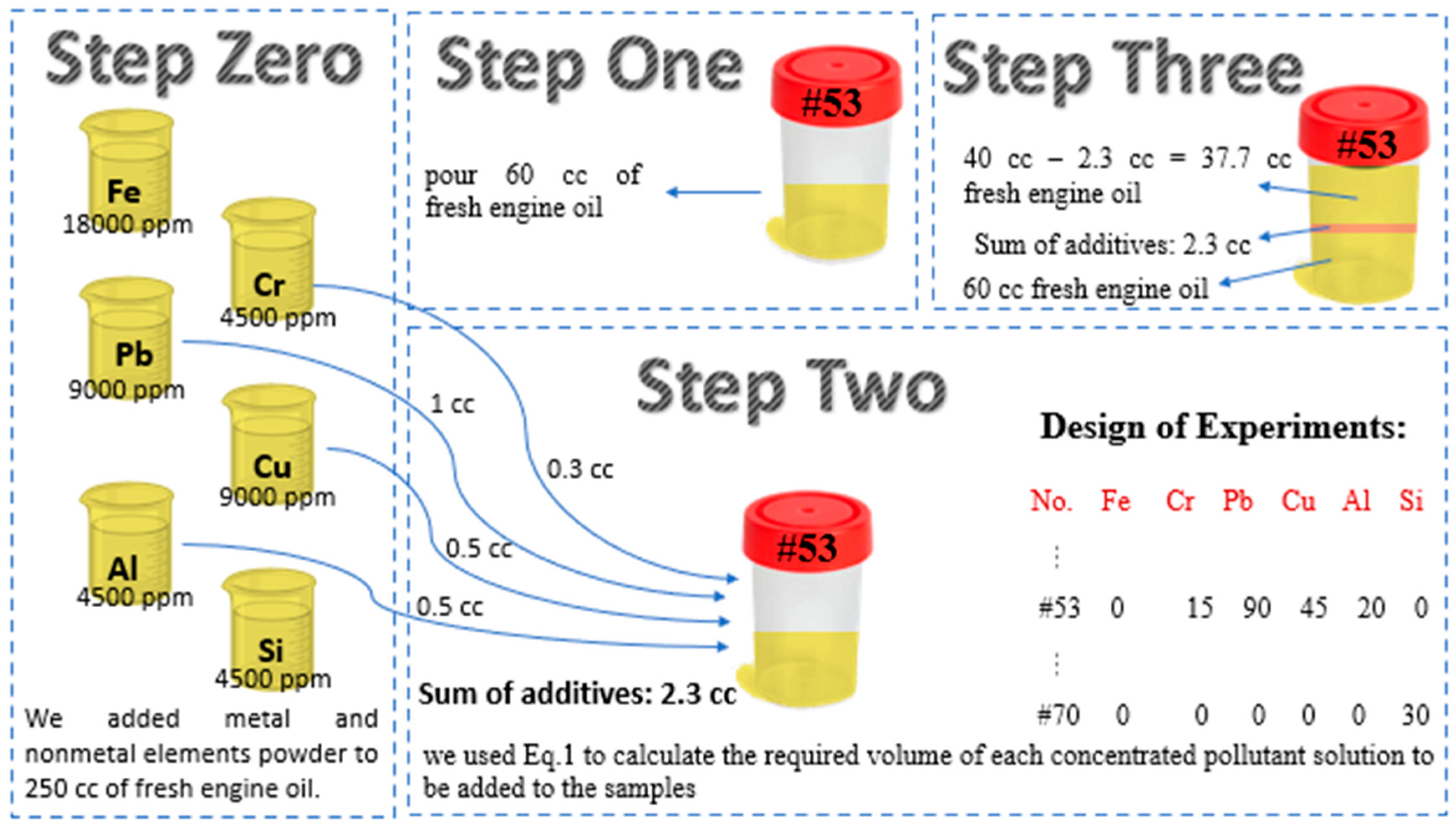
2.1. Sample Preparation

The primary objective of this study is to examine the influence of six metallic and non-metallic elements (Fe, Cr, Pb, Cu, Al, Si) on the quality of Behran Super Pishtaz 20W50 engine oil, a brand made in Iran, under normal, cautious, and critical conditions. We will achieve this by analyzing the changes in the electrical properties (ε′, ε″, tan δ) of the engine oil. The engine oil used in this examination met the following specs:

• Viscosity at 100 °C was equal to 19.5 cSt based on ASTM D445 test [55].
• Flash point was equal to 228 °C according to ASTM D92 test [56].
• Pour point was equal to −27 °C based on ASTM D97 test [57].
• Density was equal to 884 kg/m³ according to ASTM D4052 test [58].
• Total alkalinity was equal to 7.5 mg KOH/g based on ASTM D2896 test [59].

In this study, based on research sources and experiences [4,41,54,60,61,62,63,64,65], we have narrowed down the pollutants to six metallic and non-metallic elements. These elements were chosen due to their significant influence on engine oil quality. A Design of Experiments (DoE) approach, specifically the Box–Behnken Design (BBD) method [66,67], was employed to design experiments. This statistical approach allowed us to reduce the number of samples [68] while considering the interaction effects of the six influential pollutants (Fe, Cr, Pb, Cu, Al, Si) at three levels: normal, cautious, and critical. We acknowledge that our study did not explicitly explore the interactions between the selected elements. However, by utilizing the Box–Behnken Design (BBD) test plan, we were able to systematically vary the conditions under which the elements were present or absent, creating a comprehensive set of combinations. This approach allowed us to develop a more robust model that can capture a wider range of scenarios, ultimately contributing to a better understanding of the relationships between the elements and their impact on engine performance. We have prepared 53 samples using the Design of BBD experiments, with 6 factors and 5 center points in one block (

Table 2. Six studied variables and levels.

Unit	Factors	Actual and Coded Values
		−1	0	1
ppm	Fe	0	125	250
	Cr	0	15	30
	Pb	0	45	90
	Cu	0	45	90
	Al	0	20	40
	Si	0	30	60
cc *	Fe	0	0.7	1.4
	Cr	0	0.3	0.6
	Pb	0	0.5	1.0
	Cu	0	0.5	1.0
	Al	0	0.5	1.0
	Si	0	0.7	1.4

*: The provided values represent the volume to be removed from the concentrated contaminated samples and added to each sample, following the design of experiment (DOE).

). Additionally, we have included 6 single pollutant samples with a caution pollutant level, 6 single pollutant samples with a critical pollutant level, and 5 fresh oil samples without pollutants to make the study more comprehensive. While 70 samples (53 + 6 + 6 + 5) may not be sufficient to develop a practical neural network in real-world applications, it is common in academic research to use neural networks with smaller datasets. In fact, other studies have successfully applied neural networks with as few as 29 [69], 33 [53], and 49 [54] samples. In this study, we also worked with 70 samples and addressed the issue of generalizability to ensure that our results are reliable and trustworthy.

Finally, the compounds of pollutants for these 70 oil samples were determined. The volume of each sample was standardized at 100 cc. The sample preparation process is as follows (Figure 2):

Step zero: Considering the small concentration of pollutants and the small volume of each sample, we first prepared very concentrated samples of each pollutant. An ultrasonic stirrer was used to maintain the dispersion of the powder pollutants in the concentrated samples. To prepare the concentrated pollutant samples, we followed these steps for each of the six metallic and non-metallic elements:

• High Fe concentration (approximately 18,000 ppm): We added 4 g of Fe powder to 250 cc of fresh engine oil.
• High Cr concentration (approximately 4500 ppm): We added 1 g of Cr powder to 250 cc of fresh engine oil.
• High Pb concentration (approximately 9000 ppm): We added 2 g of Pb powder to 250 cc of fresh engine oil.
• High Cu concentration (approximately 9000 ppm): We added 2 g of Cu powder to 250 cc of fresh engine oil.
• High Al concentration (approximately 4500 ppm): We added 1 g of Al powder to 250 cc of fresh engine oil.
• High Si concentration (approximately 4500 ppm): We added 1 g of Si powder to 250 cc of fresh engine oil.

In the following:

Step one: First, to avoid rework, pour 60 cc of fresh engine oil into the sample container.

Step two: Next, we used Equation (1) [70] to calculate the required volume of each concentrated pollutant solution to be added to the samples, to achieve the expected concentration of each pollutant in the 100 cc volume.

$$a_1{v}_1=a_2{v}_2$$

(1)

In this context, $a_1$ and $v_1$ represent the concentration and volume of the first sample, respectively. Similarly, $a_2$ and $v_2$ denote the concentration and volume of the second sample.

Step three: Subtract the total volume of pollutants added to each sample from 40 cc. This will give us the volume of fresh engine oil that must be added to each sample to make the total volume equal to 100 cc.

2.2. Electrical Measurement

In this study, we investigate the dielectric properties of lubricant oil samples containing various pollutants at different concentrations. The dielectric properties, particularly the real (ε′) and imaginary (ε″) parts of the dielectric constant and the loss tangent (tan δ), are analyzed at multiple frequency points ranging from 2 to 8 GHz. The dielectric constant is a significant parameter that indicates the ability of a material to store energy compared to free space. It is influenced by factors such as frequency, temperature, mixture, orientation, and pressure [53,54].

To measure the electrical properties (ε′, ε″, tan δ) of the lubricant oil samples, we employed the N1501A Dielectric Probe Kit connected to the Keysight N9917A FieldFox Handheld Microwave Analyzer and its corresponding software. This setup allows for precise dielectric constant measurement of the lubricant samples. Before the measurements, a calibration process was performed. The probe used in the measurement process is designed for high-temperature applications. The calibration standards (Std1, Std2, and Std3) include air, a short circuit, and 18.6 °C water, respectively. The initial frequency of the baseline (IFBW) is set to 300 Hz, and the power level is adjusted to −45 dBm.

To obtain reliable and consistent results, each measurement was repeated five times for every lubricant oil sample. The values reported for each parameter, including the real and imaginary parts of the dielectric constant and the loss tangent, are the average of these five repetitions. This approach ensures that the presented data represent the average behavior of the lubricant oil samples under investigation and reduces the influence of potential measurement errors or fluctuations in the experimental setup [53,71].

By studying the dielectric properties (ε′, ε″, tan δ) of the lubricant oil samples with varying pollutant concentrations and frequencies, we aim to offer precious insights into the conduct of these pollutants in the oil and their ability to impact the electric properties (ε′, ε″, tan δ) of lubricants. This fact can contribute to the improvement of better strategies for monitoring and retaining the overall performance of lubricated systems.

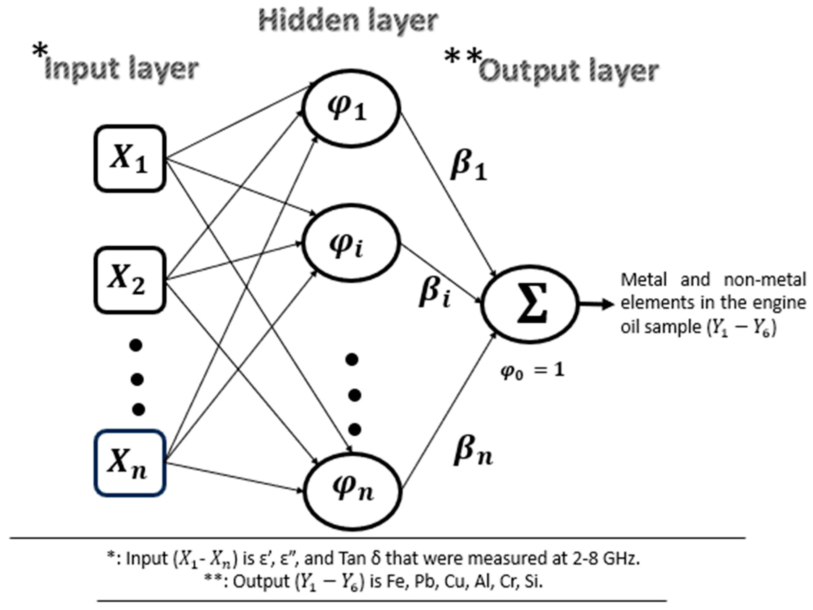
2.3. Soft Computing Modeling

In this research, we aim to predict the values of six pollutants in lubricant oil samples using five machine learning models. Five models including Radial Basis Function (RBF) [72,73], Adaptive Neuro-Fuzzy Inference System (ANFIS) [74], Multilayer Perception (MLP) [75], Gaussian Process Regression (GPR) [76], and Support Vector Machine (SVM) [77] are used in this study. These models primarily use electrical properties (ε′, ε″, tan δ) assessed at select frequency points as input data, rather than comprehensive measurements within the 2-8 GHz range. This limitation arises from the necessity to avoid overly complex models. In this context, the validation of measurements based on background, experience, and trial and error has been [53,54]. To ensure that the range of inputs does not influence the models’ performance and to assess the importance of input parameters accurately, we normalized (Equation (2)) the values of the electrical characteristics (ε′, ε″, tan δ). The normalized input values were then introduced as the input of the model, and the values of each pollutant were considered as the output of the model [78].

$$x_n={\displaystyle \frac{x-x_{min}}{x_{max}{-x}_{min}}}\times \left(r_{max}-r_{min}\right)+r_{min}$$

(2)

where x signifies the original data, x_n stands for the normalized values of inputs, x_min and x_max, represent the minimum and maximum values of the variable, respectively. The transformed variable range, considered as the optimal values for the variables, are denoted as r_max and r_min.

Figure 3 illustrates the architectural configuration of the Radial Basis Function (RBF) network, serving as a visual exemplar to facilitate a comprehensive understanding of the neural network’s performance in this research. We divided the dataset (70 samples) into a training and testing phase. In this process, 80% of the data was used for training the models (56 samples), and the remaining 20% was allocated for testing their performance (14 samples). This approach allows us to assess the models’ accuracy in estimating pollutant concentrations and their ability to generalize across different samples.

In RBF, the cumulative outputs of the nonlinear activation functions, in conjunction with the weight vector of the output layer (β), yield each individual output generated by the network, which is subsequently determined by Equation (3):

$$f\left(x\right)=\sum _{i=0}^n{\beta }_i{\phi }_i$$

(3)

where ${\beta }_i$ denotes the aggregate weight coefficient of the basis function. The Gaussian function is employed as the radial basis, which is mathematically defined as:

$${\phi }_i=exp\left(-{\displaystyle \frac{{‖x-c_i‖}^2}{{\sigma }_i^2}}\right)$$

(4)

To identify the most effective model among the five, we analyzed their performance using Root-Mean-Squared Error (RMSE) (Equation (5)) [79,80] and Coefficient of Determination (R²) (Equation (6)) [81,82] indices. Once the superior model was determined, we proceeded to analyze and optimize its parameters, such as the hidden size and training algorithm, to estimate each pollutant individually.

$$RMSE=\sqrt{{\displaystyle \frac{{\sum }_{i=1}^n{(y_{pi}-y_{ei})}^2}{n}}}$$

(5)

$$R^2={\left[{\displaystyle \frac{{\sum }_{i=1}^n(y_{ei}-\overline{y_{ei}})\times (y_{pi}-\overline{y_{pi}})}{{\sum }_{i=1}^n(y_{ei}-\overline{y_{ei}})\times {\sum }_{i=1}^n(y_{pi}-\overline{y_{pi}})}}\right]}^2$$

(6)

In this context, $y_{ei}$ is the component of the desired (actual) output for the ith pattern, and $y_{pi}$ is the component of the predicted (fitted) output produced by the network for the i pattern. The $n$ is the number of lubricant samples.

To further evaluate the generalization ability of the superior model, we conducted a sensitivity analysis. In this step, we studied the changes in RMSE and R² indices as we varied the size of the training set. The training set sizes were set to 80, 70, 60, and 50, allowing us to better understand the model’s performance under different data availability scenarios. Thereby providing valuable information for future research and potential improvements in the modeling process. All matters related to programming and analysis have been performed using MATLAB R 2019a software. This choice was made due to its robust capabilities in handling machine learning algorithms and data processing. In statistical fields, we utilized Minitab 21 software, which offers a comprehensive suite of tools for data analysis and interpretation.

3. Results and Discussion

This section presents the findings of our study, focusing on the performance comparison of five machine learning models (RBF, ANFIS, MLP, GPR, and SVM) for predicting the concentrations of six pollutants (Fe, Cr, Pb, Cu, Al, and Si) in lubricant oil samples. The evaluation was based on the Root-Mean-Squared Error (RMSE) and the Coefficient of Determination (R²) for both training and testing datasets. Additionally, this section explores the optimization of superior model parameters and their generalization capabilities. These predictions and models are established upon the electrical properties (ε′, ε″, tan δ) of lubricants. The electrical characteristics were measured in 2 to 8 GHz, but the model inputs were restricted to electrical characteristics measured in three frequencies (4.64, 4.76, and 5.9 GHz). This limitation is due to validation and experiences, as well as trial-and-error processes. It is also to prevent the excessive complexity of the model.

Table 3. Inputs and output of modeling for Fe.

No	Model	Input: X									Output: Y1–Y6 *
		4.64 GHz			4.76 GHz			5.9 GHz
		X1	X2	X3	X4	X5	X6	X7	X8	X9
1	RBF	ε′	ε″	tan δ	ε′	ε″	tan δ	ε′	ε″	tan δ	Y1: Fe
2	ANFIS	ε′	ε″	tan δ	ε′	ε″	tan δ	ε′	ε″	tan δ	Y1: Fe
3	MLP	ε′	ε″	tan δ	ε′	ε″	tan δ	ε′	ε″	tan δ	Y1: Fe
4	GPR	ε′	ε″	tan δ	ε′	ε″	tan δ	ε′	ε″	tan δ	Y1: Fe
5	SVM	ε′	ε″	tan δ	ε′	ε″	tan δ	ε′	ε″	tan δ	Y1: Fe

* Y1–Y6: Y1 (Fe), Y2 (Cr), Y3 (Pb), Y4 (Cu), Y5 (Al), Y6 (Si).

illustrates the inputs utilized for predicting Fe, and it should be noted that the same input data-set was applied across all models for the prediction of the remaining pollutants (Cr, Pb, Cu, Al, and Si). This consistent approach across the five models underscores the reliability and relevance of our predictive analysis.

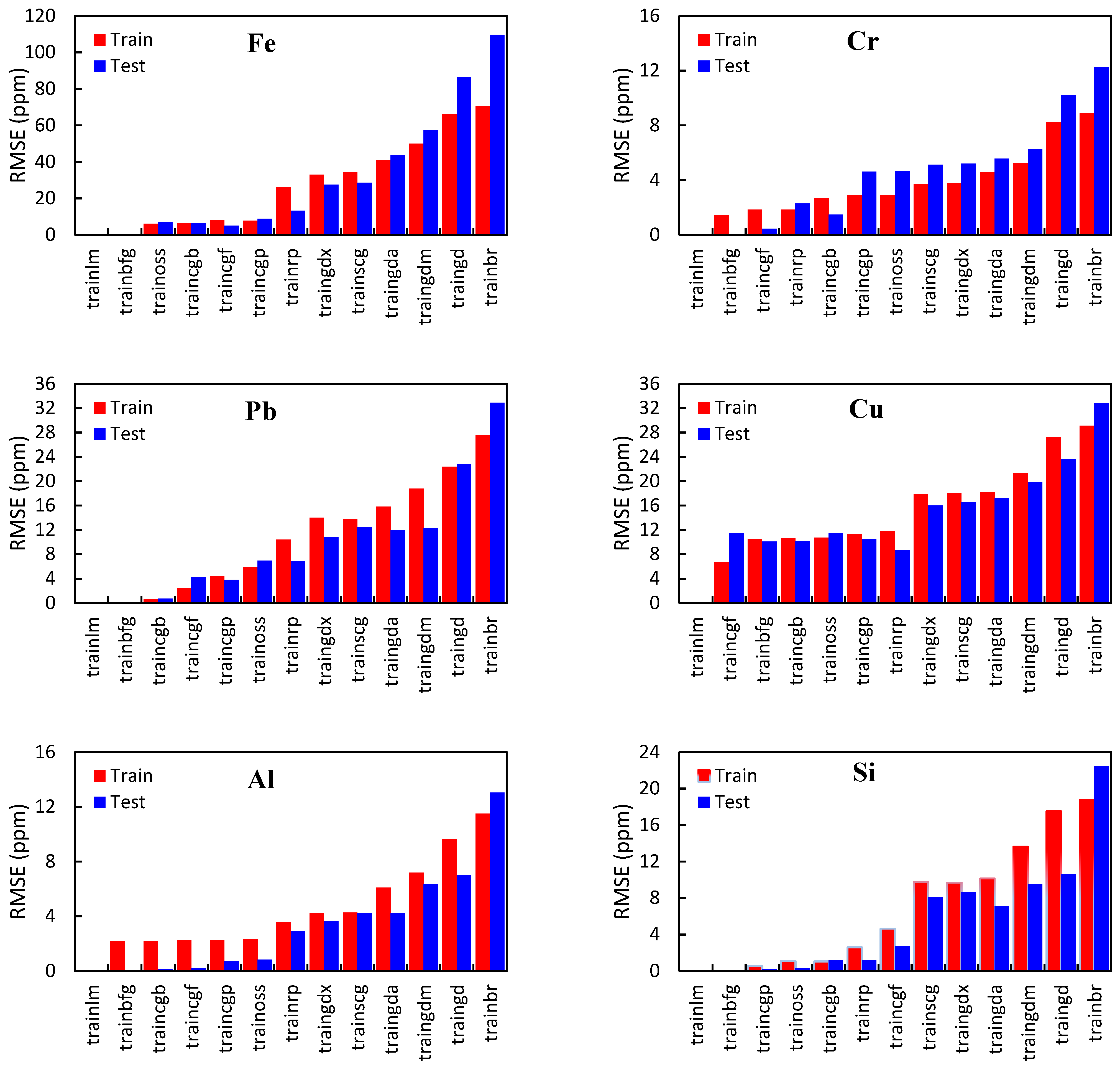
3.1. Performance Comparison of Models

This study compared the overall performance of five machine learning models—RBF, ANFIS, MLP, GPR, and SVM—for predicting the concentrations of six pollutants (Fe, Cr, Pb, Cu, Al, and Si) in lubricant oil samples. The models’ overall performance turned into evaluation by the use of two metrics: Root-Mean-Squared Error (RMSE) and Coefficient of Determination (R²). The effects are offered inside

Table 4. The performance of various models in predicting each of the pollutants.

	Model	Train		Test		All
		RMSE	R2	RMSE	R2	RMSE	R2
Fe	RBF	0.01	0.99	0.01	0.99	0.01	0.99
	ANFIS	1.67	0.99	0.85	0.99	1.54	0.99
	MLP	78.15	0.22	92.85	0.14	81.3	0.20
	GPR	78.13	0.22	90.92	0.17	80.85	0.21
	SVM	69.39	0.38	109.07	0.19	78.94	0.25
Cr	RBF	0.01	0.99	0.01	0.99	0.01	0.99
	ANFIS	0.24	0.99	0.15	0.99	0.22	0.99
	MLP	9.13	0.33	11.06	0.20	9.54	0.24
	GPR	9.19	0.32	10.52	0.08	9.47	0.25
	SVM	7.56	0.54	14.71	0.12	9.43	0.26
Pb	RBF	0.01	0.99	0.01	0.99	0.01	0.99
	ANFIS	0.24	0.99	0.15	0.99	0.22	0.99
	MLP	24.88	0.46	27.83	0.06	25.50	0.40
	GPR	29.66	0.23	32.69	0.29	30.29	0.15
	SVM	23.20	0.53	27.38	0.09	24.10	0.46
Cu	RBF	0.01	0.99	0.01	0.99	0.01	0.99
	ANFIS	0.35	0.99	0.02	0.99	0.32	0.99
	MLP	30.14	0.17	30.92	0.04	30.30	0.15
	GPR	30.49	0.15	31.54	0.01	30.70	0.12
	SVM	25.01	0.43	50.18	0.54	31.68	0.07
Al	RBF	0.01	0.99	0.01	0.99	0.01	0.99
	ANFIS	0.11	0.99	0.01	0.99	0.10	0.99
	MLP	13.44	0.19	13.59	0.13	13.47	0.15
	GPR	13.02	0.24	16.01	0.57	13.67	0.12
	SVM	11.54	0.41	15.67	0.50	12.48	0.27
Si	RBF	0.01	0.99	0.01	0.99	0.01	0.99
	ANFIS	0.19	0.99	0.04	0.99	0.17	0.99
	MLP	17.98	0.39	17.17	0.05	17.82	0.34
	GPR	16.43	0.49	16.84	0.01	16.51	0.43
	SVM	17.56	0.42	28.70	0.05	20.28	0.14

, with every row representing a distinct pollutant and the columns displaying the models’ overall performance in terms of RMSE and R² for the training dataset (Train), testing dataset (Test), and overall dataset (All).

According to Table 4, comparing the models’ overall performance for every pollutant, we see that the Radial Basis Function (RBF) model was able to predict the values of all six impurities with first-rate overall performance. The Root-Mean-Squared Error (RMSE) for all pollution in all 3 steps (training, testing, and overall) was equal to 0.01, indicating a very low prediction mistake Moreover, the Coefficient of Determination (R²) for all pollution in all three steps became equal to 0.99, signifying a sturdy relationship between the expected and real values. The Artificial Neural Network-based Adaptive Network-based Fuzzy Inference System (ANFIS) model showed reasonable overall performance for most pollutants, except for Cu and Al, where it underperformed compared to different models. The Multi-Layer Perception (MLP) model validated various overall performances throughout pollution, with some pollution (e.g., Fe, Cr, and Al) showing fantastically higher outcomes, while others (e.g., Pb, Cu, and Si) had higher RMSE and lower R² values. The Gaussian Process Regression (GPR) model additionally confirmed mixed outcomes, with a few pollutants (e.g., Fe, Cr, and Al) performing better and others (e.g., Pb, Cu, and Si) showing higher RMSE and lower R² values. The Support Vector Machine (SVM) version displayed various overall performances across pollutants as well, with some pollution (e.g., Fe, Cr, and Al) showing noticeably better results, while others (e.g., Pb, Cu, and Si) had higher RMSE and lower R² values.

In conclusion, the RBF model verified the high-quality standard overall performance for predicting the concentrations of the six pollutants in lubricant oil samples. The other models, while showing varying degrees of success, provide alternative approaches for future research and comparison. Further optimization and validation of these models, as well as incorporating additional factors affecting the dielectric properties of lubricants, can lead to improved understanding and monitoring of pollutants in lubricated systems.

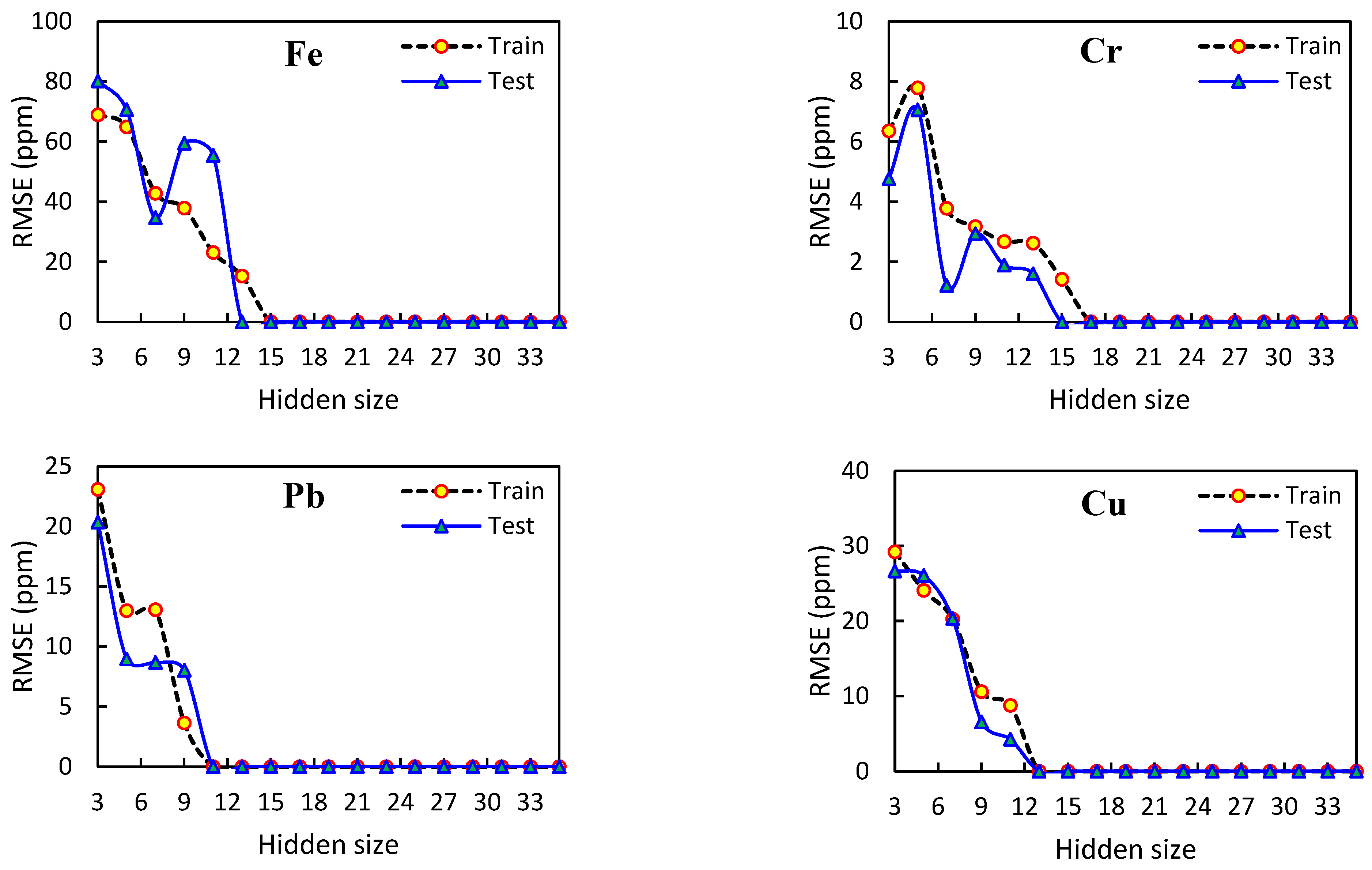
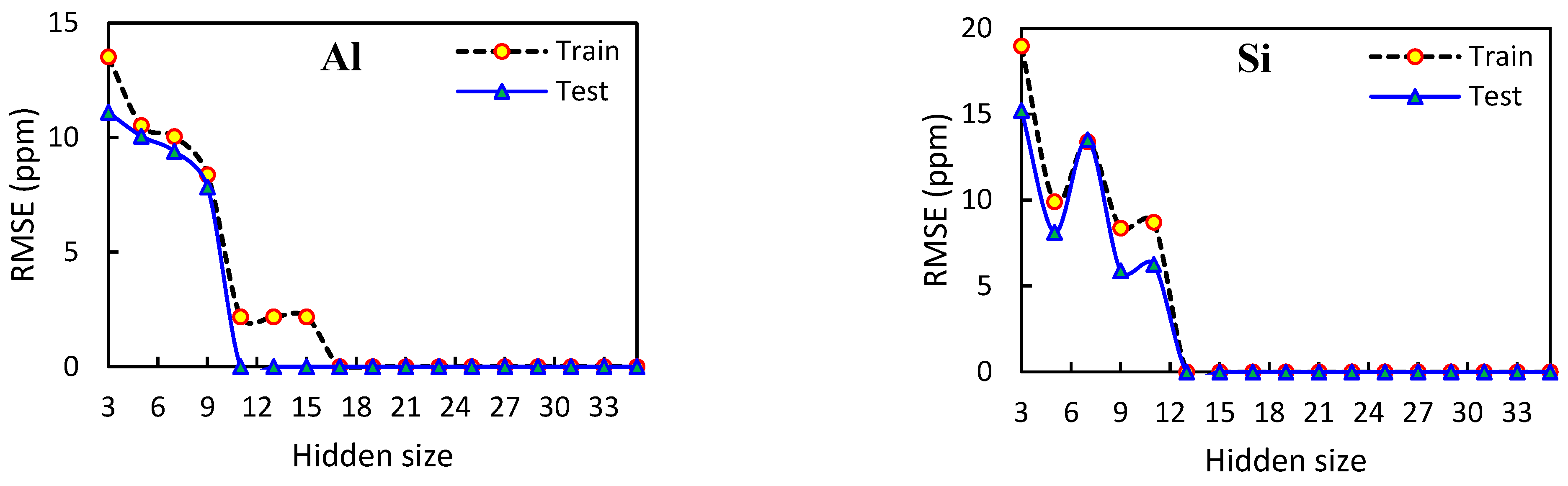
3.2. Optimizing Superior Model Parameters: Findings and Recommendations

In this section, we aimed to evaluate and optimize the parameters of the best machine learning model for predicting the content material of six pollutants (Fe, Cr, Pb, Cu, Al, and Si) using electric properties (ε′, ε″, tan δ). According to Section 3.1, upon implementing and educating the models using the dataset, we detected various performances in phrases of Root-Mean-Squared Error (RMSE) and the Coefficient of Determination (R²) at the training and testing sets. The RBF model consistently exhibited the lowest RMSE and highest R² values, demonstrating its superiority in predicting pollutant content. The RBF model’s outstanding performance can be attributed to its ability to capture complex relationships between the input features and the target variables. For the sake of continuity and brevity in the article, the linear relationship between the actual and predicted values is included in Appendix A, Figure A1.

The impact of varying hidden sizes on the RBF model’s performance, as measured by the RMSE index, is individually reported for the prediction of each pollutant (Figure 4). In predicting Fe content using electrical properties, the best-hidden size for the RBF model was found to be 15, as it resulted in zero RMSE on both the training and testing sets. In terms of predicting Cr and Al contents through electrical properties, the optimal hidden size for the RBF model was identified as 17, as it led to zero RMSE on both the training and testing datasets. When predicting Pb content using electrical properties, the RBF model’s best-performing hidden size was found to be 11, as it achieved zero RMSE on both the training and testing datasets. In the context of predicting Cu and Si contents through electrical properties, the RBF model demonstrated its best performance with a hidden size of 13, resulting in zero RMSE on both the training and testing datasets. Finally, analyzing the plots in Figure 4, it is evident that a hidden size of 17 is suitable for estimating all six pollutants using the RBF model. This conclusion is drawn from the observed zero RMSE for testing and training datasets in this configuration.

To further analyze the RBF model’s performance, we examined the effect of the Spread parameter on the RMSE values for each pollutant. We implemented a systematic approach (empirical method) to determine the optimal value of Spread parameter by conducting multiple network tests on data collected from all trials. This empirical method allowed us to analyze the performance of various Spread parameter values and select one that best suited our findings. The results are offered in Figure 5. The evaluation of the Spread parameter’s effect on the RBF model’s performance for predicting Fe content material was primarily based on the electrical characteristics (ε′, ε″, tan δ) of lubricants, which reveals that increasing the Spread parameter from a small value (e.g., 0.05) to a larger value (e.g., 0.1 or 0.2) can cause higher model overall performance. However, for higher Spread values, the model seems to obtain the best prediction, as indicated via zero RMSE values on both the training and testing steps. So, for Fe, the optimal Spread value was found to be 0.3 or greater, resulting in zero RMSE on both the training and testing sets. Similar to the analysis of the Fe prediction, the Spread parameter’s effect on the RBF model’s performance for predicting chromium content based on the electrical characteristics of lubricants shows that increasing the Spread parameter leads to improved model performance. As the Spread parameter value increases, the RMSE values on both the training and testing sets decrease, eventually reaching zero, which indicates perfect prediction for chromium content. Of course, for Cr, the optimal Spread value was found to be 0.2 or greater, resulting in zero RMSE on both the training and testing sets. Similar to the analysis of the Fe and Cr prediction, the Spread parameter’s effect on the RBF model’s performance for predicting lead content based on the electrical characteristics of lubricants shows that increasing the Spread parameter leads to improved model performance. The RMSE values on both the training and testing set decrease as the Spread parameter value increases and perfect prediction is achieved for lead content when the Spread parameter is 0.3 or greater. The spread parameter’s effect on the RBF model’s performance for predicting copper content based on the electrical characteristics of lubricants shows that as the Spread parameter increases from 0.05 to 0.1, the RMSE values on both the training and testing sets decrease, indicating improved model performance. When the Spread parameter further increases to 0.2, the RMSE values on both the training and testing sets increase. For Spread values greater than or equal to 0.3, the RMSE values on both the training and testing sets decrease, showing that the RBF model’s performance gets better at predicting Cu content. Perfect prediction (RMSE = 0) is achieved for Cu content when the Spread parameter is set to 0.4 or greater. The spread parameter’s effect on the RBF model’s performance for predicting Al content based on the electrical characteristics of lubricants shows that when the Spread parameter further increases to 0.2, the RMSE values on both the training and testing sets decrease significantly, showing that the RBF model’s performance gets much better at predicting aluminum content. For Spread values greater than or equal to 0.3, the RMSE values become zero, suggesting that the RBF model achieves perfect prediction for Al content with these parameter settings. The spread parameter’s effect on the RBF model’s performance for predicting silicon content based on the electrical characteristics of lubricants shows that when the Spread parameter increases to 0.2, the RMSE values on both the training and testing sets decrease significantly, showing that the RBF model’s performance gets much better at predicting silicon content. For Spread values equal to 0.3, the RMSE value on the training set decreases, but on the testing set increases. Perfect prediction (RMSE = 0) is maintained for Si content when the Spread parameter is set to 0.4 or greater.

The training algorithm is another effective parameter in modeling with RBF. In this part, we will examine the effect of the value of this parameter on the performance of the RBF model to estimate each of the six pollutants based on the performance index RMSE (Figure 6). The RMSE values for the “trainlm” and “trainbfg” algorithms are zero in both the training and testing stages, indicating excellent performance in estimating Fe, Pb, and Si contents using the RBF model. The “trainlm” method seems to have the best prediction performance for the Cr, Cu, and Al variables, with 0.00 RMSE in both train and test sets. Finally, based on the RMSE performance index, the “trainlm” method also performs exceptionally well for all six pollutants. This method showcases zero RMSE in the training and testing stages, indicating its strong predictive capabilities.

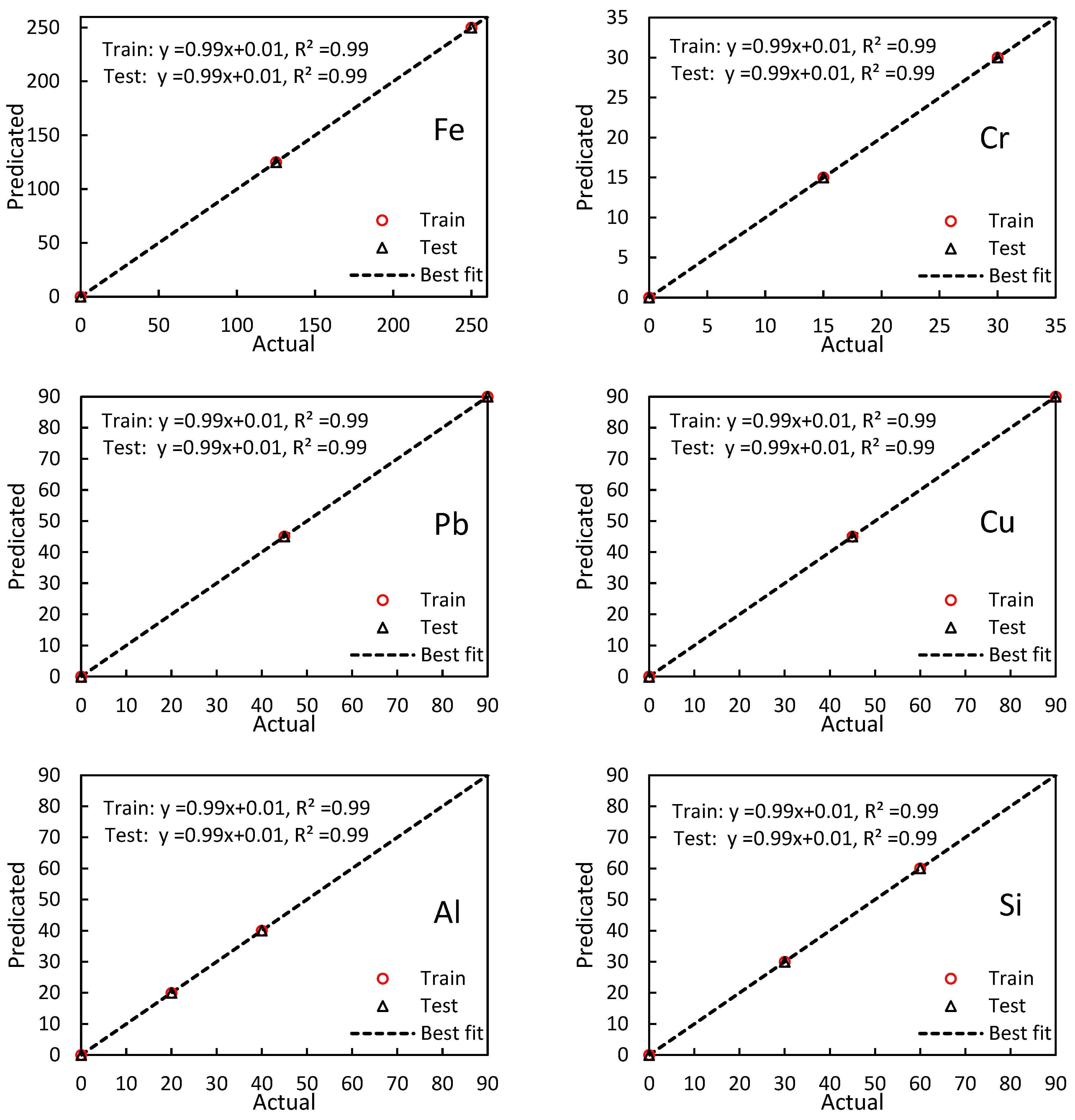
3.3. Model Generalization Capability

In this section, we investigated the performance of the Radial Basis Function (RBF) model for predicting the concentrations of Fe, Cr, Pb, Cu, Al, and Si in lubricants using electric characteristics (ε′, ε″, tan δ) of lubricants. The RBF model’s ability to generalize was evaluated by examining its performance on varying training-to-testing ratios, including 80:20, 70:30, 60:40, and 50:50 (

Table 5. The outcomes of the model’s generalizability by adjusting the ratio of training and testing sizes for each pollutant.

Model	Train Size (%)	Train		Test		All
		RMSE	R2	RMSE	R2	RMSE	R2
Fe	80	0.01	0.99	0.01	0.99	0.01	0.99
	70	0.01	0.99	0.01	0.99	0.01	0.99
	60	0.01	0.99	0.01	0.99	0.01	0.99
	50	0.01	0.99	0.01	0.99	0.01	0.99
Cr	80	0.01	0.99	0.01	0.99	0.01	0.99
	70	0.01	0.99	0.01	0.99	0.01	0.99
	60	0.01	0.99	0.01	0.99	0.01	0.99
	50	0.01	0.99	0.01	0.99	0.01	0.99
Pb	80	0.01	0.99	0.01	0.99	0.01	0.99
	70	0.01	0.99	0.01	0.99	0.01	0.99
	60	0.01	0.99	0.01	0.99	0.01	0.99
	50	0.01	0.99	0.01	0.99	0.01	0.99
Cu	80	0.01	0.99	0.01	0.99	0.01	0.99
	70	0.01	0.99	0.01	0.99	0.01	0.99
	60	7.76	0.95	14.10	0.77	10.76	0.89
	50	9.22	0.93	14.00	0.78	11.85	0.87
Al	80	0.01	0.99	0.01	0.99	0.01	0.99
	70	0.01	0.99	0.01	0.99	0.01	0.99
	60	0.01	0.99	0.01	0.99	0.01	0.99
	50	0.01	0.99	0.01	0.99	0.01	0.99
Si	80	0.01	0.99	0.01	0.99	0.01	0.99
	70	0.01	0.99	0.01	0.99	0.01	0.99
	60	0.01	0.99	0.01	0.99	0.01	0.99
	50	0.01	0.99	0.01	0.99	0.01	0.99

).

According to Table 5, the model’s overall performance is measured by the usage of the Root-Mean-Squared Error (RMSE) and the coefficient of determination (R²). The outcomes exhibit that the RBF version reveals splendid overall performance in predicting the concentrations of all six factors (Fe, Cr, Pb, Cu, Al, and Si) within the lubricants, as indicated by the constantly low RMSE and high R² values throughout all training-to-testing data ratios. This strong performance is maintained across various ratios, suggesting the model’s robustness and generalization capabilities. Of course, As the ratio decreased to 60:40 and 50:50, the model did not maintain its strong performance in estimating Cu. For example, whilst the ratio reached 50:50, the model’s overall performance degraded, with an RMSE of 11.85 and an R² of 0.87 within the All step. These results spotlight the importance of checking the degree of generalizability of the proposed model because, by doing so, the validity of the modeling procedure and the acquire d effects turn out to be extra transparent, which is vital for real-world programs and the broader acceptance of the proposed model. The findings of this have a look at how it can contribute to the development of more accurate and reliable methods for monitoring and controlling pollutants in lubricants, ultimately enhancing their overall performance and lifespan.

3.4. Comparison with Background

In a recent study [53], a comprehensive analysis of 33 oil samples extracted from locomotive diesel engines was conducted. The values of Fe, Pb, Cu, Cr, Al, Si, and Zn were measured for each sample, followed by the determination of values ε′, ε″, tan δ at four frequencies of 2.4, 5.8, 7.4, and 9.6 GHz. A neural network was employed to predict the values ε′, ε″, tan δ of each oil sample based on the measured values of Fe, Pb, Cu, Cr, Al, Si, and Zn. The results indicated that the best prediction for values ε′, ε″, tan δ was achieved at a frequency of 7.4 GHz.

In another study [54], a dataset of 49 oil samples extracted from diesel engines was analyzed. The values of Fe, Pb, Cu, Cr, Al, Si, and Zn were collected for each sample, followed by the calculation of values ε′, ε″, tan δ at three frequencies of 2.4, 5.8, and 7.4 GHz. Five neural network models (RBF, MLP, ANFIS, GPR, SVM) were employed to predict the values of Fe, Pb, Cu, Cr, Al, Si, and Zn of each oil sample based on the calculated values of ε′, ε″, tan δ. The results showed that the best prediction was achieved at a frequency of 7.4 GHz using the RBF model.

In this current research, a Box–Behnken design (BBD) scheme was employed to contaminate 70 oil samples with six metallic and non-metallic impurities: Fe, Pb, Cu, Cr, Al, and Si. The values of ε′, ε″, tan δ for each sample were measured at three frequencies of 4.64, 4.76, and 5.9 GHz. Five neural network models (RBF, ANFIS, MLP, GPR, and SVM) were employed to predict the values of Fe, Pb, Cu, Cr, Al, and Si of each oil sample based on the measured values of ε′, ε″, tan δ at three frequencies. The results indicated that the RBF model made the best prediction for the six metallic and non-metallic impurities.

The performance of the RBF model was improved in this study by predicting Fe, Pb, Cu, Cr, Al, and Si in each oil sample. The Root-Mean-Squared Error (RMSE) value for predicting Fe, Pb, Cu, Cr, Al, and Si by RBF was found to be 0.01. In contrast, previous study [54] reported an RMSE value ranging from 0.1 to 2.2. This improvement in performance may be attributed to the fact that in this study, nine input parameters (values of ε′, ε″, tan δ at three frequencies) were used in the RBF model compared to only three input parameters (values of ε′, ε″, tan δ at one frequency) used in previous study [54]. Additionally, the laboratory contamination of oil samples in this study allowed for more precise measurement of electrical properties without interference from other factors such as oxidation caused by working time.

In conclusion, this study highlights the importance of selecting appropriate input parameters for neural network models in predicting metal and non-metal impurities in oil samples. The results demonstrate that the RBF model can be effectively used to predict impurities in oil samples when trained with a comprehensive set of input parameters.

4. Conclusions

In summary, this academic study aimed to investigate the impact of six metallic and non-metallic elements (Fe, Cr, Pb, Cu, Al, Si) on the quality of Behran Super Pishtaz 20W50 engine oil under varying conditions. A Design of Experiments (DoE) approach, specifically the Box–Behnken Design (BBD) method, was employed to design experiments, resulting in 70 engine oil samples being analyzed for their electrical properties (ε′, ε″, tan δ) in the frequency range of 2 to 8 GHz.

The performance of five machine learning models (RBF, ANFIS, MLP, GPR, and SVM) was assessed in predicting the concentration of these six pollutants based on the electric characteristics (ε′, ε″, tan δ) of the lubricant. The Radial Basis Function (RBF) model demonstrated great performance, as indicated by low Root-Mean-Squared Error (RMSE) and high R² values in each of the training and testing steps.

Optimization of the RBF model’s parameters revealed an optimal hidden size of 17, which led to zero RMSE for most pollutants in both the training and testing datasets. Additionally, the study found that higher Spread values (0.4 or greater) positively influenced the RBF model’s performance in predicting pollutant content. The study’s findings also emphasize the effectiveness of the “trainlm” training algorithm in achieving zero RMSE for all six pollutants in both the training and testing phases. The RBF model demonstrates splendid overall performance in predicting concentrations of Fe, Cr, Pb, Cu, Al, and Si throughout numerous training-to-testing ratios (80:20, 70:30, 60:40, and 50:50), as evidenced by way of continually low Root-Mean-Squared Error (RMSE) and high coefficient of determination (R²) values. However, the model’s overall performance in estimating Cu concentrations degrades while the ratio decreases to 60:40 and 50:50. These findings emphasize the importance of checking the model’s generalization capabilities for increased confidence in its predictions.

This research contributes to a better understanding of the behavior of pollutants in lubricants and their potential impact on lubricant electrical properties (ε′, ε″, tan δ). The findings can be applied to various industries relying on lubricants, such as automotive, aviation, and manufacturing, to enhance maintenance strategies and overall equipment efficiency. The developed RBF model can be integrated into predictive maintenance systems, enabling real-time monitoring of lubricant quality and preventing unexpected equipment breakdowns, thereby reducing maintenance costs and improving overall productivity. Furthermore, the results of this study can contribute to the development of industry standards and regulatory guidelines for lubricant quality assurance.

Future research directions may involve incorporating additional factors affecting the dielectric properties of lubricants, optimizing machine learning models further, and validating the results using real-world data. Ensuring the reproducibility of this method and addressing limitations, such as the necessity of obtaining accurate equipment and high-quality cables to minimize noise, is crucial. Incorporating fuzzy logic into future research could enhance our ability to model the interactions among various elements and their contributions to oil quality. It can allow for a more nuanced analysis by accommodating the uncertainty in measurements and the subjective nature of certain parameters, such as the quality indicators we assessed. For example, fuzzy logic can offer a way to interpret the complex relationships between pollutant concentrations and their impact on electrical properties, potentially improving predictive accuracy and reliability.

Additionally, exploring the development of disposable equipment or testing methods, similar to rapid blood sugar test strips, for probing lubricants can enhance the accessibility and efficiency of monitoring lubricant quality. By addressing these challenges and expanding the scope of research, the field of lubricant quality assessment can significantly contribute to maintaining and improving the performance of critical systems across various industries.

References

1. Xin, Q. Diesel Engine System Design; Elsevier: Amsterdam, The Netherlands, 2011. [Google Scholar]
2. Ernst, R.J.; Pefley, R.K.; Wiens, F.J. Methanol Engine Durability; 0148-7191; SAE Technical Paper; SAE International: Warrendale, PA, USA, 1983. [Google Scholar]
3. Cyrus, J.D. Engine component life prediction methodology for conceptual design investigations. In Turbo Expo: Power for Land, Sea, and Air; American Society of Mechanical Engineers: New York, NY, USA, 1986. [Google Scholar]
4. Nieto, P.G.; García-Gonzalo, E.; Lasheras, F.S.; de Cos Juez, F.J. Hybrid PSO–SVM-based method for forecasting of the remaining useful life for aircraft engines and evaluation of its reliability. Reliab. Eng. Syst. Saf. 2015, 138, 219–231. [Google Scholar] [CrossRef]
5. Piancastelli, L.; Frizziero, L.; Marcoppido, S.; Pezzuti, E. Methodology to evaluate aircraft piston engine durability. Int. J. Heat Technol. 2012, 30, 89–92. [Google Scholar]
6. Deng, K.; Zhang, X.; Cheng, Y.; Zheng, Z.; Jiang, F.; Liu, W.; Peng, J. A remaining useful life prediction method with long-short term feature processing for aircraft engines. Appl. Soft Comput. 2020, 93, 106344. [Google Scholar] [CrossRef]
7. Zaman, M.; Siswantoro, N.; Priyanta, D.; Pitana, T.; Prastowo, H.; Busse, W. The combination of reliability and predictive tools to determine ship engine performance based on condition monitoring. In Proceedings of the IOP Conference Series: Earth and Environmental Science, Surakarta, Indonesia, 24–25 August 2021; p. 012015. [Google Scholar]
8. Cao, D.; Bai, G. A study osn aeroengine conceptual design considering multi-mission performance reliability. Appl. Sci. 2020, 10, 4668. [Google Scholar] [CrossRef]
9. Loiselle, R.; Xu, Z.; Voloh, I. Essential motor health monitoring: Making informed decisions about motor maintenance before a failure occurs. IEEE Ind. Appl. Mag. 2018, 24, 8–13. [Google Scholar] [CrossRef]
10. Glavaš, H.; Kljajin, M.; Desnica, E. Essential Preventive Automobile Maintenance during a Pandemic. Teh. Vjesn. 2021, 28, 2190–2199. [Google Scholar]
11. Hutchings, I.; Shipway, P. Tribology: Friction and Wear of Engineering Materials; Butterworth-Heinemann: Oxford, UK, 2017. [Google Scholar]
12. Lin, H.-H.; Heinze, J.; Croy, A.; Gutiérrez, R.; Cuniberti, G. Effect of lubricants on the rotational transmission between solid-state gears. Beilstein J. Nanotechnol. 2022, 13, 54–62. [Google Scholar] [CrossRef]
13. Rahim, K.A.; Al-Humairi, S.N.S. Influence of Lubrication Technology on Internal Combustion Engine Performance: An Overview. In Proceedings of the 2020 IEEE 8th Conference on Systems, Process and Control (ICSPC), Melaka, Malaysia, 11–12 December 2020; pp. 184–189. [Google Scholar]
14. Grassart, P. Monitoring of the Lubrication System of an Aircraft Engine through a Prognostic and Health Monitoring Approach. Master’s Thesis, KTH School of Industrial Engineering and Management, Stockholm, Sweden, 2015. [Google Scholar]
15. Domínguez-García, S.; Béjar-Gómez, L.; López-Velázquez, A.; Maya-Yescas, R.; Nápoles-Rivera, F. Maximizing Lubricant Life for Internal Combustion Engines. Processes 2022, 10, 2070. [Google Scholar] [CrossRef]
16. Bulgakov, N.; Kovalenko, V.; Gorbaneva, A.; Shalimov, S. Management of preventive maintenance of vehicles. In Proceedings of the IOP Conference Series: Materials Science and Engineering, Kazimierz Dolny, Poland, 21–23 November 2019; p. 012074. [Google Scholar]
17. Figueredo, G.P.; Owa, K.; John, R. Multi-objective optimization for time-based preventive maintenance within the transport network: A review. Acad. Libr. Comput. 2020. [Google Scholar] [CrossRef]
18. Ventikos, N.P.; Sotiralis, P.; Annetis, E. A combined risk-based and condition monitoring approach: Developing a dynamic model for the case of marine engine lubrication. Transp. Saf. Environ. 2022, 4, tdac020. [Google Scholar] [CrossRef]
19. Vališ, D.; Žák, L.; Pokora, O. Failure prediction of diesel engine based on occurrence of selected wear particles in oil. Eng. Fail. Anal. 2015, 56, 501–511. [Google Scholar] [CrossRef]
20. Kučera, M.; Kopčanová, S.; Sejkorová, M. Lubricant analysis as the most useful tool in the proactive maintenance philosophies of machinery and its components. Manag. Syst. Prod. Eng. 2020, 28, 196–201. [Google Scholar] [CrossRef]
21. Ganiboyeva, E.; Khakimov, B.; Shermuxamedov, X.; Rakhimov, Y. Theoretical study of the accumulation of mechanical mixtures in the engine lubrication system. IOP Conf. Ser. Earth Environ. Sci. 2022, 1076, 012085. [Google Scholar] [CrossRef]
22. Heredia-Cancino, J.; Ramezani, M.; Álvarez-Ramos, M. Effect of degradation on tribological performance of engine lubricants at elevated temperatures. Tribol. Int. 2018, 124, 230–237. [Google Scholar] [CrossRef]
23. Srinivasan, U.; Muthuveerappan, N.; Sudhindra, K. Development of Data Prediction Model for the Lubrication System in a Developmental Gas Turbine Engine. J. Aerosp. Sci. Technol. 2020, 1–8. [Google Scholar] [CrossRef]
24. Rahman, M.H.; Shahriar, S.; Menezes, P.L. Recent Progress of Machine Learning Algorithms for the Oil and Lubricant Industry. Lubricants 2023, 11, 289. [Google Scholar] [CrossRef]
25. Zhu, J.; Yoon, J.M.; He, D.; Qu, Y.; Bechhoefer, E. Lubrication oil condition monitoring and remaining useful life prediction with particle filtering. Int. J. Progn. Health Manag. 2013, 4, 124–138. [Google Scholar] [CrossRef]
26. He, M.; He, D.; Yoon, J.; Nostrand, T.J.; Zhu, J.; Bechhoefer, E. Wind turbine planetary gearbox feature extraction and fault diagnosis using a deep-learning-based approach. Proc. Inst. Mech. Eng. Part O J. Risk Reliab. 2019, 233, 303–316. [Google Scholar] [CrossRef]
27. Kornaeva, E.; Kornaev, A.; Kazakov, Y.N.; Polyakov, R. Application of artificial neural networks to diagnostics of fluid-film bearing lubrication. In Proceedings of the IOP Conference Series: Materials Science and Engineering, Chennai, India, 16–17 September 2020; p. 012154. [Google Scholar]
28. Afzal, A.B.; Jain, U.; Khan, N.A. Condition Monitoring of Dielectrics. In Proceedings of the 2018 3rd International Innovative Applications of Computational Intelligence on Power, Energy and Controls with their Impact on Humanity (CIPECH), Ghaziabad, India, 1–2 November 2018; pp. 221–226. [Google Scholar]
29. Gogoi, N.; Chen, J.; Kirchner, J.; Fischer, G. Dependence of piezoelectric discs electrical impedance on mechanical loading condition. Sensors 2022, 22, 1710. [Google Scholar] [CrossRef]
30. Palomino, L.V.; Steffen Jr, V.; de Moura, J.d.R.V.; Tsuruta, K.M.; Rade, D.A. Impedance-based health monitoring and mechanical testing of structures. Smart Struct. Syst. Int. J. 2011, 7, 15–25. [Google Scholar] [CrossRef]
31. Fiorenza, P.; Greco, G.; Di Franco, S.; Giannazzo, F.; Monnoye, S.; Zielinski, M.; La Via, F.; Roccaforte, F. Electrical properties of thermal oxide on 3C-SiC layers grown on silicon. In Materials Science Forum; Trans Tech Publications Ltd.: Wollerau, Switzerland, 2019; pp. 479–482. [Google Scholar]
32. Torreblanca González, J.; García Ovejero, R.; Lozano Murciego, Á.; Villarrubia González, G.; De Paz, J.F. Effects of environmental conditions and composition on the electrical properties of textile fabrics. Sensors 2019, 19, 5145. [Google Scholar] [CrossRef] [PubMed]
33. Li, J.; Ding, Q.; Wang, H.; Wu, Z.; Gui, X.; Li, C.; Hu, N.; Tao, K.; Wu, J. Engineering Smart Composite Hydrogels for Wearable Disease Monitoring. Nano-Micro Lett. 2023, 15, 105. [Google Scholar] [CrossRef] [PubMed]
34. Svoboda, M.; Harvánek, L. Online Monitoring and Lifetime Estimations of Materials for Electrical Insulation. In Proceedings of the 2015 IEEE 11th International Conference on the Properties and Applications of Dielectric Materials (ICPADM), Sydney, Australia, 19–22 July 2015; pp. 568–571. [Google Scholar]
35. Kumar, S.; Mukherjee, P.; Mishra, N. Online condition monitoring of engine oil. Ind. Lubr. Tribol. 2005, 57, 260–267. [Google Scholar] [CrossRef]
36. Chun, S.M. Analysis of Test Results for Small Dipstick-Gage-Type Engine-Oil-Deterioration-Detection Sensor. Tribol. Lubr. 2014, 30, 156–167. [Google Scholar]
37. Turner, J.; Austin, L. Electrical techniques for monitoring the condition of lubrication oil. Meas. Sci. Technol. 2003, 14, 1794. [Google Scholar] [CrossRef]
38. Vasanthan, B.; Devaradjane, G.; Shanmugam, V. Online condition monitoring of lubricating oil on test bench diesel engine & vehicle. J. Chem. Pharm. Sci. 2015, 9, 315–320. [Google Scholar]
39. Mauntz, M.; Kuipers, U.; Gegner, J. New Electric Online Oil Condition Monitoring Sensor—An Innovation in Early Failure Detection of Industrial Gears. In Proceedings of the The 4th International Multi-Conference on Engineering and Technological Innovation, Orlando, FL, USA, 19–22 July 2011; pp. 238–242. [Google Scholar]
40. Abellán-Martín, S.J.; Aguirre, M.Á.; Canals, A. Applicability of microwave induced plasma optical emission spectrometry for wear metal determination in lubricant oil using a multinebulizer. J. Anal. At. Spectrom. J. Anal. At. Spectrom. 2023, 38, 1379–1386. [Google Scholar] [CrossRef]
41. Fernández-Feal, M.; Sánchez-Fernández, L.; Pérez-Prado, J. Study of Metal Concentration in Lubricating Oil with Predictive Purposes. Curr. J. Appl. Sci. Technol. 2018, 27, 1–12. [Google Scholar] [CrossRef]
42. Han, W.; Mu, X.; Liu, Y.; Wang, X.; Li, W.; Bai, C.; Zhang, H. A Critical Review of On-Line Oil Wear Debris Particle Detection Sensors. J. Mar. Sci. Eng. 2023, 11, 2363. [Google Scholar] [CrossRef]
43. Guan, L.; Feng, X.; Xiong, G.; Xie, J. Application of dielectric spectroscopy for engine lubricating oil degradation monitoring. Sens. Actuators A Phys. 2011, 168, 22–29. [Google Scholar] [CrossRef]
44. Guan, L.; Feng, X.; Xiong, G. Engine lubricating oil classification by SAE grade and source based on dielectric spectroscopy data. Anal. Chim. Acta 2008, 628, 117–120. [Google Scholar] [CrossRef]
45. Xiao, J.; Wu, Y.; Zhang, W.; Chen, J.; Zhang, C. Friction of metal-matrix self-lubricating composites: Relationships among lubricant content, lubricating film coverage, and friction coefficient. Friction 2020, 8, 517–530. [Google Scholar] [CrossRef]
46. Ulrich, C.; Petersson, H.; Sundgren, H.; Björefors, F.; Krantz-Rülcker, C. Simultaneous estimation of soot and diesel contamination in engine oil using electrochemical impedance spectroscopy. Sens. Actuators B Chem. 2007, 127, 613–618. [Google Scholar] [CrossRef]
47. Qiang, L.; Xiaowei, L.; Lili, C.; Jiang, W. Research on a Method for the Determination of Iron in Lubricating Oil. In Proceedings of the 1st International Conference on Mechanical Engineering and Material Science (MEMS 2012), Shanghai, China, 28–30 December 2012; Atlantis Press: Zhengzhou, China, 2012; pp. 180–182. [Google Scholar]
48. Qiang, L.; Jiang, W.; Lili, C.; Xiaowei, L. A Study of Moisture Content of Lubricating Oil Based on Impedance Analysis. In Proceedings of the 1st International Conference on Mechanical Engineering and Material Science (MEMS 2012), Shanghai, China, 28–30 December 2012; Atlantis Press: Zhengzhou, China, 2012; pp. 183–186. [Google Scholar]
49. Zhou, Y.; Hao, M.; Chen, G.; Wilson, G.; Jarman, P. Frequency-dependence of conductivity of new mineral oil studied by dielectric spectroscopy. In Proceedings of the 2012 International Conference on High Voltage Engineering and Application, Shanghai, China, 17–20 September 2012; pp. 634–637. [Google Scholar]
50. Delgado, E.; Aperador, W.; Hernández, A. Impedance Spectroscopy as a Tool for the Diagnosis of the State of Vegetable Oils Used as Lubricants. Int. J. Electrochem. Sci. 2015, 10, 8190–8199. [Google Scholar] [CrossRef]
51. Chowdhury, S.R.; Kumar, R.; Kaur, R.; Sharma, A.; Bhondekar, A.P. Quality assessment of engine oil: An impedance spectroscopy based approach. In Proceedings of the 2016 IEEE Uttar Pradesh Section International Conference on Electrical, Computer and Electronics Engineering (UPCON), Varanasi, India, 9–11 December 2016; pp. 608–612. [Google Scholar]
52. Macioszek, Ł.; Włodarczak, S.; Rybski, R. Mineral oil moisture measurement with the use of impedance spectroscopy. IET Sci. Meas. Technol. 2019, 13, 1158–1162. [Google Scholar] [CrossRef]
53. Altıntaş, O.; Aksoy, M.; Ünal, E.; Akgöl, O.; Karaaslan, M. Artificial neural network approach for locomotive maintenance by monitoring dielectric properties of engine lubricant. Measurement 2019, 145, 678–686. [Google Scholar] [CrossRef]
54. Pourramezan, M.-R.; Rohani, A.; Abbaspour-Fard, M.H. Unlocking the Potential of Soft Computing for Predicting Lubricant Elemental Spectroscopy. Lubricants 2023, 11, 382. [Google Scholar] [CrossRef]
55. Ruggiero, A.; D’Amato, R.; Merola, M.; Valášek, P.; Müller, M. On the tribological performance of vegetal lubricants: Experimental investigation on Jatropha Curcas L. oil. Procedia Eng. 2016, 149, 431–437. [Google Scholar] [CrossRef]
56. Abdelkhalik, A.; Elsayed, H.; Hassan, M.; Nour, M.; Shehata, A.B.; Helmy, M. Using thermal analysis techniques for identifying the flash point temperatures of some lubricant and base oils. Egypt. J. Pet. 2018, 27, 131–136. [Google Scholar] [CrossRef]
57. Oliveira, L.M.; Nunes, R.C.; Ribeiro, Y.L.; Coutinho, D.M.; Azevedo, D.A.; Dias, J.; Lucas, E.F. Wax behavior in crude oils by pour point analyses. J. Braz. Chem. Soc. 2018, 29, 2158–2168. [Google Scholar] [CrossRef]
58. Abdurrojaq, N.; Devitasari, R.D.; Aisyah, L.; Faturrahman, N.A.; Bahtiar, S.; Sujarwati, W.; Wibowo, C.S.; Anggarani, R.; Maymuchar, M. Perbandingan Uji Densitas Menggunakan Metode ASTM D1298 dengan ASTM D4052 pada Biodiesel Berbasis Kelapa Sawit. Lembaran Publ. Miny. Gas Bumi 2021, 55, 49–57. [Google Scholar] [CrossRef]
59. Dutta, M.; Pathiparampil, A.; Murella, J.; Villacarte, D.; Hamada, D.; Hernandez, J.; Lopez-Linares, F. Determination of base number in lubricants and additives by ASTM D2896: Substitution of chlorinated solvents and alternate electrolyte study. Fuel 2021, 297, 120701. [Google Scholar] [CrossRef]
60. Li, L.; Chang, W.; Zhou, S.; Xiao, Y. An identification and prediction model of wear-out fault based on oil monitoring data using PSO-SVM method. In Proceedings of the 2017 Annual Reliability and Maintainability Symposium (RAMS), Orlando, FL, USA, 23–26 January 2017; pp. 1–6. [Google Scholar]
61. Zhou, P.; Liu, D. Research on marine diesel’s fault prognostic and health management based on oil monitoring. In Proceedings of the 2011 Prognostics and System Health Managment Conference, Shenzhen, China, 24–25 May 2011; pp. 1–4. [Google Scholar]
62. Al-Nozili, M.S.; Abeed, F.A.; Ahmed, M.M. Studying the Changes of Some Heavy Metals Content in Lubricating Oil Caused by Using; Part I: Diagnostic Study. Int. J. Emerg. Technol. Adv. Eng. 2014, 4, 396. [Google Scholar]
63. Wolak, A.; Zając, G.; Gołębiowski, W. Determination of the content of metals in used lubricating oils using AAS. Pet. Sci. Technol. 2019, 37, 93–102. [Google Scholar] [CrossRef]
64. Pourramezan, M.-R.; Rohani, A.; Keramat Siavash, N.; Zarein, M. Evaluation of lubricant condition and engine health based on soft computing methods. Neural Comput. Appl. 2022, 35, 5465–5477. [Google Scholar] [CrossRef]
65. Pourramezan, M.-R.; Rohani, A.; Abbaspour-Fard, M.H. Comparative Analysis of Soft Computing Models for Predicting Viscosity in Diesel Engine Lubricants: An Alternative Approach to Condition Monitoring. ACS Omega 2023, 9, 1398–1415. [Google Scholar] [CrossRef]
66. Rawat, A.; Jhawat, V.; Dutt, R. DoE Enabled Development and In-Vitro Optimization of Curcumin-tagged Cilostazol Solid Nano Dispersion. Curr. Nanomed. Former. Recent Pat. Nanomed. 2023, 13, 113–131. [Google Scholar] [CrossRef]
67. Palandurkar, K.; Bhandre, R.; Boddu, S.H.; Harde, M.; Lakade, S.; Kandekar, U.; Waghmare, P. Quality risk assessment and DoE–Practiced validated stability-indicating chromatographic method for quantification of Rivaroxaban in bulk and tablet dosage form. Acta Chromatogr. 2023, 35, 10–20. [Google Scholar] [CrossRef]
68. Kamani, H.; Safari, G.H.; Asgari, G.; Ashrafi, S.D. Data on modeling of enzymatic elimination of direct red 81 using response surface methodology. Data Brief 2018, 18, 80–86. [Google Scholar] [CrossRef]
69. Musa, M.A.; Chowdhury, S.; Biswas, S.; Alam, S.N.; Parvin, S.; Sattar, M.A. Removal of aqueous methylene blue dye over Vallisneria Natans biosorbent using artificial neural network and statistical response surface methodology analysis. J. Mol. Liq. 2024, 393, 123624. [Google Scholar] [CrossRef]
70. Pourramezan, E.; Omidvar, M.; Motavalizadehkakhky, A.; Zhiani, R.; Darzi, H.H. Enhanced adsorptive removal of methylene blue using ternary nanometal oxides in an aqueous solution. Biomass Convers. Biorefinery 2024, 1–13. [Google Scholar] [CrossRef]
71. An, D.; Guo, J.; Chang, X.; Wang, Z.; Jia, Y.; Liu, X.; Bondur, V.; Sun, H. High-precision 1′ × 1′ bathymetric model of Philippine Sea inversed from marine gravity anomalies. EGUsphere 2024, 17, 2039–2052. [Google Scholar] [CrossRef]
72. Seyed Ahmad Soleymani, S.A.S.; Shidrokh Goudarzi, S.G.; Mohammad Hossein Anisi, M.H.A.; Wan Haslina Hassan, W.H.H.; Mohd Yamani, I.; Shahaboddin Shamshirband, S.S.; Noorzaily Mohamed Noor, N.M.N.; Ismail Ahmedy, I.A. A novel method to water level prediction using RBF and FFA. Water Res. Manag. 2016, 30, 3265–3283. [Google Scholar] [CrossRef]
73. Szwajka, K.; Zielińska-Szwajka, J.; Trzepieciński, T. The use of a radial basis function neural network and fuzzy modelling in the assessment of surface roughness in the MDF milling process. Materials 2023, 16, 5292. [Google Scholar] [CrossRef] [PubMed]
74. Stojčić, M.; Stjepanović, A.; Stjepanović, Đ. ANFIS model for the prediction of generated electricity of photovoltaic modules. Decis. Mak. Appl. Manag. Eng. 2019, 2, 35–48. [Google Scholar] [CrossRef]
75. Borghi, P.H.; Zakordonets, O.; Teixeira, J.P. A COVID-19 time series forecasting model based on MLP ANN. Procedia Comput. Sci. 2021, 181, 940–947. [Google Scholar] [CrossRef]
76. Thapa, S.; Zhao, Z.; Li, B.; Lu, L.; Fu, D.; Shi, X.; Tang, B.; Qi, H. Snowmelt-driven streamflow prediction using machine learning techniques (LSTM, NARX, GPR, and SVR). Water 2020, 12, 1734. [Google Scholar] [CrossRef]
77. Otchere, D.A.; Ganat, T.O.A.; Gholami, R.; Ridha, S. Application of supervised machine learning paradigms in the prediction of petroleum reservoir properties: Comparative analysis of ANN and SVM models. J. Pet. Sci. Eng. 2021, 200, 108182. [Google Scholar] [CrossRef]
78. Heidari, P.; Rezaei, M.; Rohani, A. Soft computing-based approach on prediction promising pistachio seedling base on leaf characteristics. Sci. Hortic. 2020, 274, 109647. [Google Scholar] [CrossRef]
79. Masoudi, H.; Rohani, A. Citrus fruit grading based on the volume and mass estimation from their projected areas using ANFIS and GPR models. Fruits Int. J. Trop. Subtrop. Hortic. 2021, 76, 169–180. [Google Scholar] [CrossRef]
80. Abbasnia, A.; Jafari, M.; Rohani, A. A novel method for estimation of stress concentration factor of central cutouts located in orthotropic plate. J. Braz. Soc. Mech. Sci. Eng. 2021, 43, 348. [Google Scholar] [CrossRef]
81. Taki, M.; Mehdizadeh, S.A.; Rohani, A.; Rahnama, M.; Rahmati-Joneidabad, M. Applied machine learning in greenhouse simulation; new application and analysis. Inf. Process. Agric. 2018, 5, 253–268. [Google Scholar] [CrossRef]
82. Siavash, N.K.; Ghobadian, B.; Najafi, G.; Rohani, A.; Tavakoli, T.; Mahmoodi, E.; Mamat, R. Prediction of power generation and rotor angular speed of a small wind turbine equipped to a controllable duct using artificial neural network and multiple linear regression. Environ. Res. 2021, 196, 110434. [Google Scholar] [CrossRef] [PubMed]
Figure 1. The summary of the research process.
Lubricants 12 00411 g001
Figure 2. The process of preparing one of the samples of contaminated oil.
Lubricants 12 00411 g002
Figure 3. The schematic structure of the RBF network employed in this work.
Lubricants 12 00411 g003
Figure 4. The changes in the RMSE index of the model against the hidden size separately for each pollutant.
Lubricants 12 00411 g004aLubricants 12 00411 g004b
Figure 5. The changes in the RMSE index of the model against the spread parameter separately for each pollutant.
Lubricants 12 00411 g005
Figure 6. The changes in the RMSE index of the model against the training algorithm separately for each pollutant.
Lubricants 12 00411 g006