Sensitivity of TEHL Simulations to the Use of Different Models for the Constitutive Behaviour of Lubricants

Abstract

This study compares the film thickness, lubricant temperature, and traction curves of two groups of commonly used constitutive models for lubricants in thermo-elastohydrodynamic lubrication (TEHL) modelling. The first group consists of the Tait equation of state, the Doolittle Newtonian viscosity model, and the Carreau shear thinning model. The second group includes the Dowson equation of state, the Roelands–Houpert Newtonian viscosity model, and the Eyring shear thinning model. The simulations were conducted using a Computational Fluid Dynamic and Fluid-Structure Interaction (CFD-FSI) approach, which employs a homogeneous equilibrium model for the flow simulation along with a linear elastic solver to describe the deformation of the solid materials. The simulations were conducted under a load range of $100\mathrm{kN}/\mathrm{m}$ to $200\mathrm{kN}/\mathrm{m}$ and a slide-to-roll-ratio (SRR) range between $0$ and $2$ using Squalane lubricant. The results show up to a 10% deviation in central film thickness, a $31\%$ deviation in coefficient of friction (CoF), and a $38\%$ deviation in maximum lubricant temperature when using the different constitutive models. This study highlights the sensitivity of TEHL simulation results to the choice of constitutive models for lubricants and the importance of carefully selecting the appropriate models for specific applications.

1. Introduction

Thermo-elastohydrodynamic lubrication (TEHL) occurs in a variety of machine components, e.g., cam-follower contacts, bearing contacts, and gear contacts. Because of the relatively small contacts that are highly loaded, the film thickness is very small, whereas the hydrodynamic pressure can rise significantly, even up to 3 GPa. In case of significant slip and shear, the temperature may also rise significantly within the small contact. It is well known that there is a significant variation in the properties of the lubricant under these conditions. In the past 50 years, several constitutive equations have been developed to describe the dependency of lubricant properties on the governing conditions in TEHL contacts. These equations have been used in numerical modelling to evaluate pressure and temperature distributions, film thicknesses, and to calculate friction. It is well known that constitutive models for viscosity and density are crucial to obtain proper results from the numerical modelling of TEHL contacts.

In brief, there are three so-called equations of state developed by Dowson, Tait, and Murnaghan which link the density to the pressure. Dowson and Higginson obtained a compressibility model from curve-fitting data of mineral oils as a function of pressure up to about $400\mathrm{MPa}$ for a given temperature [1]. Note that Tait’s equation is an empirical model, whereas Murnaghan’s equation is derived from a linear theory of finite strain [2].

Besides density, viscosity also plays an essential role in (T)EHL. There are mainly three mechanisms impacting the viscosity, i.e., piezo-viscous behaviour, temperature dependency, and shear thinning behaviour. Typically, the pressure and temperature effects are taken into account through a Newtonian viscosity model, whereas a non-Newtonian model is required when shear rates are high, e.g., when sliding occurs. The Roelands model is the most commonly used Newtonian viscosity model [3]. This empirical correlation was reported to be valid at least up to $400 \mathrm{MPa}$ and between 20–50 °C for general mineral oils. Doolittle, on the other hand, developed a model based on free-volume theory for liquid viscosity and suggested using the free volume, related to density, as an input variable for viscosity calculation instead of using temperature and pressure directly [4]. A free-volume model states that the relative volume of molecules present in a liquid affects the resistance to flow. Note that these models have been modified several times to be adopted for the TEHL problem [5,6,7].

At high shear rates, liquid lubricants display a non-Newtonian behaviour, particularly shear thinning, implying that the viscosity decreases with increasing shear rate. Johnson and Tevaarwerk [8] investigated the fluid shear behaviour in the EHL oil film and proposed the original form of the Eyring model. They found a broad agreement between the non-linear Maxwell model and Eyring theory when the pressure and temperature variation were taken into account. The Eyring model has often been used in classical EHL calculation. However, in some recent studies, the non-Newtonian Carreau shear thinning model has been preferred [9,10,11]. It has been proven that the sinh law or Eyring model can predict the traction curve accurately according to the traction test of Conry et al. [12]. Note that this study specifically investigated the traction curve for LVI260 oil. However, Bair reported different properties of LVI260, especially the viscosity and shear modulus [7]. Furthermore, Bair et al. [13] argued that the viscosity data should be fitted to the rheological flow curve (viscosity vs. shear rate) to predict both traction and film thickness accurately and not to the traction curve. Furthermore, the basics and assumptions behind these shear thinning models are reviewed by Spike and Jie [14]. They stated that input parameters in the Eyring and Carreau models greatly affect the accuracy of these models; both models could predict accurately when their parameters were tuned. However, Bair et al. [15] objected to this, pointing to some misrepresentations in the work of Spike and Jie.

Kumar and Khonsari [16] compared the Eyring (sinh law) and power law-based Carreau models. They showed that the Carreau model could predict central film thickness more successfully in the EHL point contact. They also showed that the traction curve is more sensitive to the value of the pressure-viscosity coefficient. In a recent study, Tosic et al. [17] employed the CFD-Boussinesq approach to investigate more in-depth the differences between the two sets of constitutive models mentioned earlier. They indicate that the choice of constitutive models becomes more crucial at higher loads. However, Tosic et al. applied a very low Eyring stress value for Squalane in their comparison, which can considerably influence the evaluation of the final TEHL solution.

Although the combination of Dowson, Roelands, and Eyring models was typically used in classical EHL calculations, the combination of Tait, Doolittle, and Carreau models has recently received more attention. Despite the fact that all of these models claim to be accurate, there is still some debate about their accuracy and the fundamental differences between them [14,15]. Although several studies have mainly focused on the differences in the prediction of viscosity, mean shear stress, and traction curve [18,19,20,21], the actual sensitivity of TEHL solutions and derived parameters to the chosen constitutive models for the same lubricant have not been investigated in-depth and will be the focus of this paper.

The classical Reynolds approach has been extensively used to investigate the importance of using reliable rheological models [22,23,24]. This approach has been proven to be accurate and efficient for EHL contact under isothermal conditions. Nevertheless, the Reynolds approach, albeit a modified version, is also used for non-isothermal EHL calculations and requires coupling with an energy equation to calculate thermal transport along and across the lubricant film and in the solids. An additional complication is that the Reynolds equation requires integration over the film thickness of the lubricant properties, which are temperature-dependent. Alternatively, one can solve the complete set of conservation equations, i.e., mass, momentum, and energy, using CFD in combination with constitutive equations to describe the dependency of lubricant properties to state variables and shear rate, avoiding the use of complicated integral of the properties across the film thickness. It goes without saying that CFD involves much more computing time and resources but with the gain of offering potentially more in-depth insight into local physical phenomena [25].

Almqvist and Larsson [26], in their pioneering work, opted to solve the Navier–Stokes equations instead of the Reynolds equation to simulate TEHL contacts. They used a single-phase CFD model, which involved solving equations for mass and momentum conservation, as well as an energy equation. They successfully simulated TEHL contact with a maximum contact pressure of $0.7\mathrm{GPa}$. Hartinger et al. [27] were one of the first to model a 2D line TEHL contact using CFD. They have found a significant pressure gradient across the lubricant film in sliding conditions, which is mainly due to the viscosity gradient induced by the temperature gradient across the film thickness. A thermal validation of this model for 3D point TEHL contact was presented later [28]. Hajishafiee et al. [29] extended Hartinger’s model to include a linear elastic structural model for the solid body as well as a robust and two-way FSI coupling model, which is more appropriate for high loads. Scurria et al. [30] compared the Reynolds equation and the full Navier–Stokes equation for EHL contact under isothermal conditions for Newtonian lubricants. They observed that the inertia term influenced the accuracy of the Reynolds solution, especially at low loads and relatively high speeds of rotation.

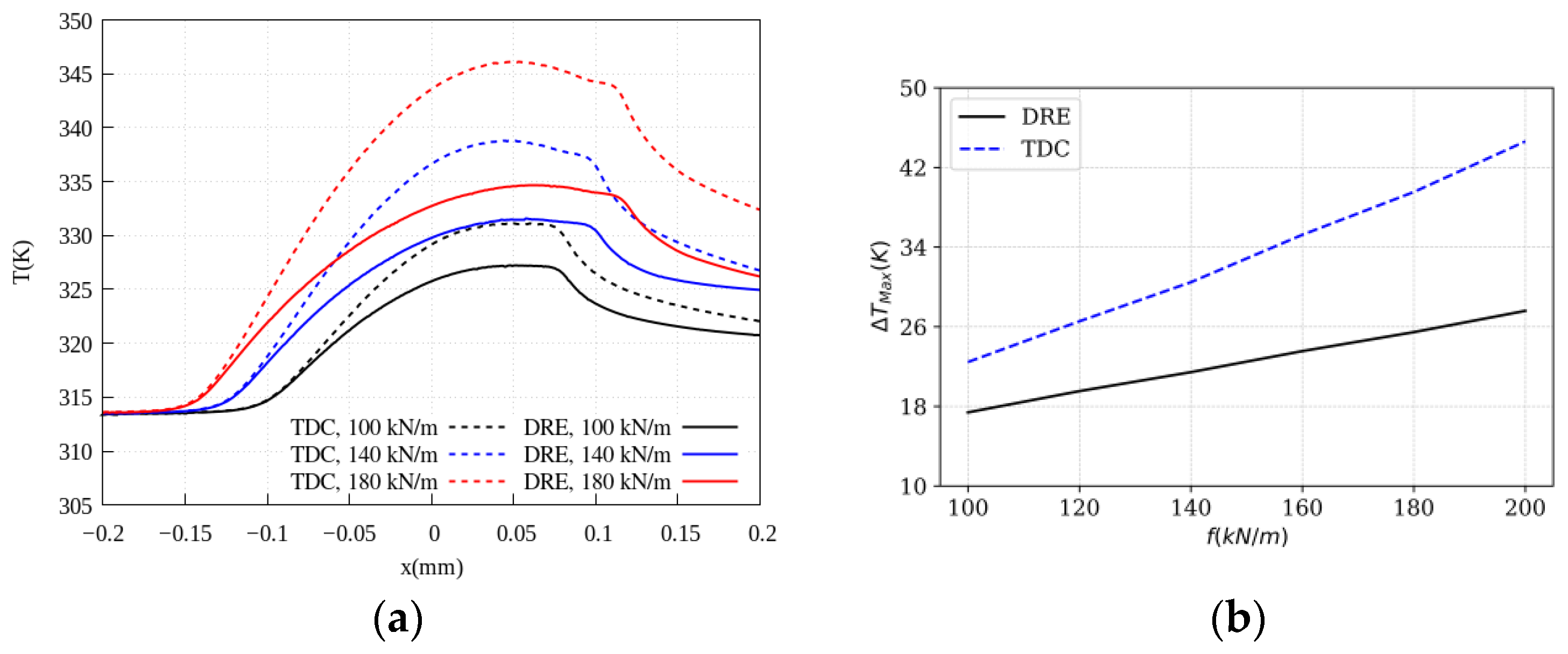
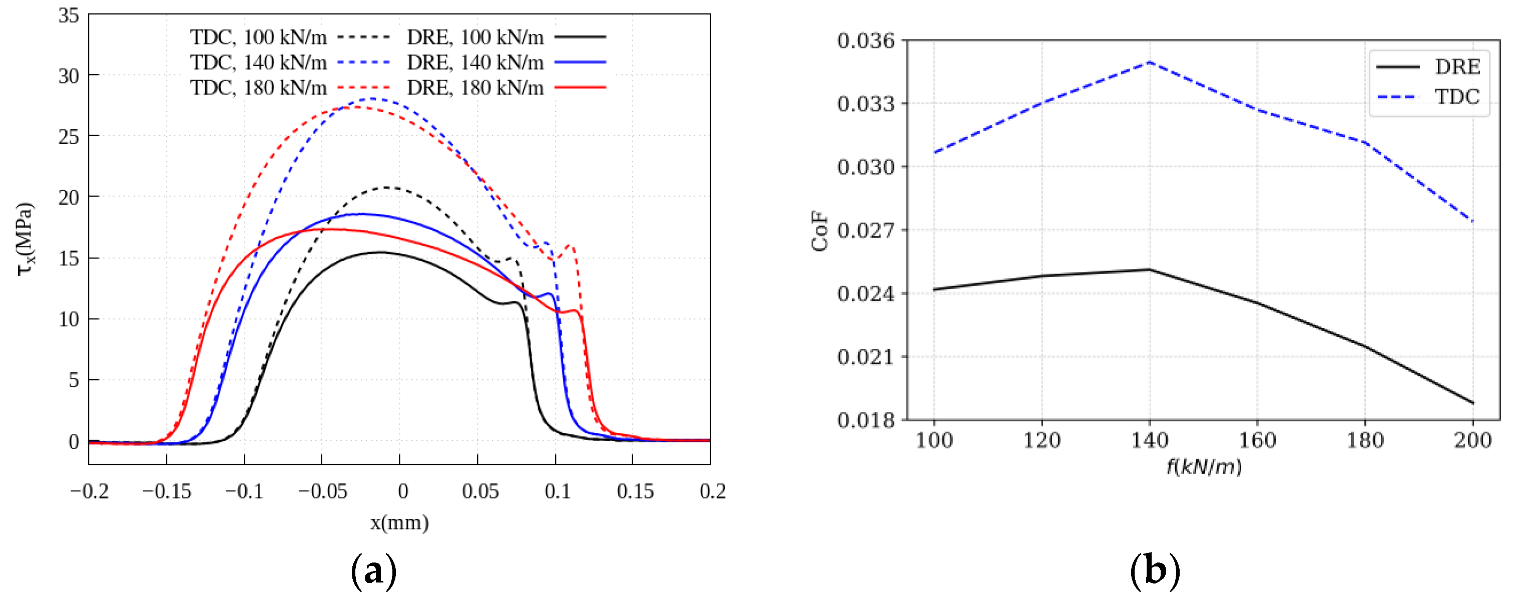
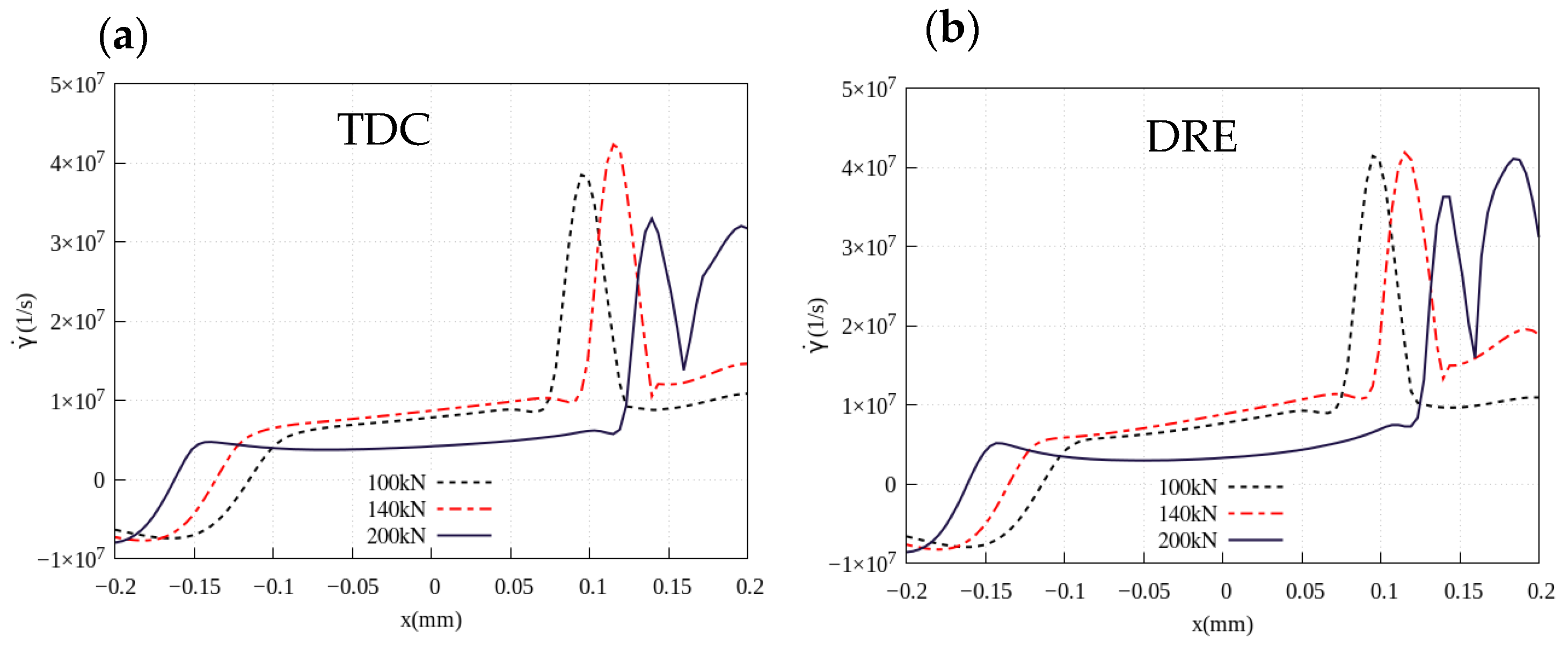
In this paper, the authors aim to compare the film thickness, lubricant temperature, and traction curve of the aforementioned two groups of well-known constitutive models, commonly used together, under different operating conditions. Thereto the CFD-FSI approach is used to avoid effects of film thickness averaging of lubricant properties. The first group includes the Dowson model for the density and the Roelands and Eyring models for viscosity. The second group includes the Tait model for density combined with the Doolittle and Carreau models for viscosity. A homogeneous equilibrium model (HEM) is used to describe cavitation, and the above-mentioned advanced constitutive models are implemented and applied. Moreover, a linear elastic solver in combination with a temperature equation is employed to describe deformation and heat conduction through the solid materials. The numerical results will fundamentally be evaluated to provide a clear picture for comparing these models. Moreover, the deviations between predicted contact variables, e.g., film thickness, temperature, coefficient of friction, etc., will be quantified for these well-known lubricant constitutive equations under a wide range of operating conditions.

2. 2D TEHL CFD-FSI Model

We consider a 2D line contact formed by a cylinder and a rigid flat plate, as presented in Figure 1. The lubricant is entrained and pressurized in the converging zone, generating a high pressure at the contact region and separating both surfaces while taking up the load. Note that due to recirculation at the inlet, a shear heating phenomenon is observed there, increasing heat transfer between contact and inlet region, which can be captured precisely by means of CFD modelling [31]. By contrast, at the outlet region, the pressure drops suddenly, and cavitation occurs.

2.1. Fluid Equations of Motion

To precisely incorporate the compressibility and phase change of lubricant at the outlet region, a combination of a Homogeneous Equilibrium Model (HEM) with a barotropic Equation of State (EoS) has been employed [32]. All governing equations for fluid motion are listed in

Table 1. Fluid equations of motion.

Description	Equation
Mass conservation	$\frac{\partial \rho }{\partial t}+\nabla \cdot (\rho \overrightarrow{u})=0$	(1)
Momentum equation	$\frac{\partial (\rho \overrightarrow{u})}{\partial t}+\nabla \cdot (\rho \overrightarrow{u}\overrightarrow{u})-\nabla \cdot \tau =-\nabla \cdot p$	(2)
Viscous stress tensor	$\tau =\mu (\nabla \overrightarrow{u}+{(\nabla \overrightarrow{u})}^T)-\mu \frac{2}{3}I\nabla \cdot \overrightarrow{u}$	(3)
Energy equation	$\rho C_p\frac{DT}{Dt}+\frac{D{\alpha }_v}{Dt}({\rho }_v{h}_v-{\rho }_l{h}_l)=\nabla \cdot (k_{eff} \nabla T)-\tau :\nabla \overrightarrow{u}+{\alpha }_v\frac{DP}{Dt}+{\alpha }_l\beta T\frac{DP}{Dt}$	(4)
Mixture density	$\rho =\psi (p-p_{sat})+{\alpha }_l{\rho }_{l,0}+({\alpha }_v{\psi }_v+{\alpha }_l{\psi }_{l,M})p_{sat}$	(5)
Vapor volume fraction	${\alpha }_v=\frac{\rho -{\rho }_{l,sat}}{{\rho }_{v,sat}-{\rho }_{l,sat}}$	(6)
Mixture compressibility	$\psi ={\alpha }_v{\psi }_v+{\alpha }_l{\psi }_{l,M}$	(7)
Vapor density	${\rho }_v={\psi }_{v}p$	(8)
Liquid density	${\rho }_l={\rho }_{l,0}+{\psi }_{l,M}p$	(9)
Liquid average compressibility	${\psi }_{l,M}(p,T)=\frac{1}{p-p_{sat}}{{\displaystyle \int }}_{p_{sat}}^p{\psi }_l(p^{\prime },T)d{p}^{\prime }=\frac{1}{p-p_{sat}}{{\displaystyle \int }}_{p_{sat}}^p{(\frac{\partial {\rho }_l}{\partial p^{\prime }})}_{s}d{p}^{\prime }$	(10)

, including the conservation of mass, momentum, and energy. It should be pointed out that the mixture dynamic viscosity, heat capacity, and compressibility is assumed to be a linearly weighted average of both phase fractions. Although the phase change is primarily governed by a decrease in pressure, despite the name barotropic EoS, temperature effects are included in phase density; hence, the density depends on both pressure and temperature. Regarding the energy equation, Equation (4) has been used for the mixture temperature based on the studies of Hartinger et al. [27,28,33] and Hajishafiee [29,34].

2.2. Solid Equations

In order to calculate stresses and deformation in a solid body, the well-known Navier–Cauchy equation for moderate stresses and strains is used, which is provided in

Table 2. Solid equations [34].

Description	Equation
Navier–Cauchy equation	${\rho }_s\frac{{\partial }^2(\overrightarrow{v})}{\partial t^2}-\nabla \cdot \left[{\mu }_s\nabla \overrightarrow{v}+{\mu }_s{(\nabla \overrightarrow{v})}^T+{\lambda }_{s}I(tr(\nabla \overrightarrow{v}))\right]={\rho }_s\overrightarrow{f_b}$	(11)
Lame coefficients	${\mu }_s=\frac{E}{2(1+\vartheta )}$	(12)
	${\lambda }_s=\frac{\vartheta E}{(1+\vartheta )(1-2\vartheta )}$	(13)
Heat conduction in the moving solid	${\rho }_s{C}_s\frac{\partial T}{\partial t}+\dot{\overrightarrow{v}.}\nabla T=\nabla \cdot (k_s \nabla T)$	(14)

. Note that heat conduction in the moving solid materials is presented in Equation (14), which is solved along with the fluid energy conservation equation to obtain the solid temperature field.

The external load ($f_{ext}$) exerted on the contact pair should be balanced by the hydrodynamic load resulting from the generated pressure in the lubricant film, which is calculated by integrating the pressure over the roller surface ($f={\displaystyle \int }p.\overrightarrow{e_n}dA)$. To ensure that the load balance is satisfied, the proper rigid displacement of the rigid plate is calculated iteratively using Equation (15).

$$\Delta h_d=\left({\left|v\right|}_{max}-{\left|v\right|}_{min}\right)\frac{f_{ext}-f}{f_{ext}} \frac{\Delta t}{t_d} r_d$$

(15)

where $\Delta h_d$ is the increment in rigid displacement calculated in each iteration, $t_d=\raisebox{1ex}{$R$}\!\left/ \!\raisebox{-1ex}{$a_s$}\right.$ is a characteristic deformation time, $a_s$ is the sonic velocity in the solid material, $r_d$ is an under-relaxation factor, and ${\left|v\right|}_{max}$ and ${\left|v\right|}_{min}$ are the maximum and minimum deformation in the solid body, respectively [29,34].

2.3. Boundary Conditions

For the rigid wall sliding over the contact, the Carslaw–Jaeger temperature boundary condition is used, which has been suggested for TEHL contacts [35,36]. It has been derived for a moving point heat source for a semi-infinite body. In a 2D line contact, the temperature is

$$T_{Cars}=\sqrt{\frac{1}{\pi {\rho }_s{c}_s{k}_s{u}_s}}{{\displaystyle \int }}_{-\infty }^x{q}_f\left(\widehat{x}\right)\frac{d\widehat{x}}{\sqrt{x-\widehat{x}}}$$

(16)

This boundary can be used for Peclet number greater than 5, $Pe=\frac{L_{ch}{u}_s}{{\alpha }_T}>5$, which is fully satisfied in this study. Note that $L_{ch}$ is the characteristic length of contact, and ${\alpha }_T=\frac{k_s}{{\rho }_s{c}_s}$ is the thermal diffusivity coefficient in solid materials.

In this work, the energy equation has been solved for the equivalent deformable body. However, it becomes computationally more expensive for the rigid plate to solve the heat conduction equation. Hence, the Carslaw–Jaeger boundary condition is preferred for the rigid plate. It is worth noting that the calculated Peclet number for the studied cases falls between 18 and 35.

The fluid and structural solvers have been developed in the OpenFOAM-extend framework to simulate the hydrodynamic and thermal behaviour of 2D and 3D TEHL contacts. The solids4Foam toolbox developed by Cardiff et al. [37] has also been used to benefit from existing fluid–structure interaction models. Furthermore, all partial differential equations were discretized by the Finite Volume Method (FVM).

A partitioned approach has been applied to couple the fluid and solid solvers, in which the interface displacement is determined using an Aitken algorithm [37]. In this two-way FSI coupling, the displacement is transferred from the solid to the fluid domain using Aitken relaxation, whereas the pressure and shear forces are transferred from the fluid to the solid domain without modification. A brief overview of the interface coupling procedure is presented in Algorithm 1. We emphasize that this algorithm works perfectly for TEHL simulation, and it only requires between 3 to 8 FSI coupling iterations to achieve convergence up to 10⁻⁸. Moreover, the temperature and heat flux are transferred between regions properly to guarantee a continuous temperature field across the interface.

Algorithm 1 CFD-FSI Algorithm

Initialize all fluid and solid fields from the previous time step

Update load balance and rigid plate location

While $\parallel r^k{\parallel }_2>{\epsilon }_0$ do          ⊳ r is displacement residual, and ε0 is the tolerance

Calculate interface relaxation factor using the Aitken algorithm (ωk)

Adjust displacement ($x_f^{k+1}=x_f^k+$ ωkrk)  ⊳ xf is the displacement of the interface at the fluid domain

Update fluid geometry

Solve flow equations

Transfer pressure and traction forces from fluid to solid

Solve structural equations ($x_s^{k+1}$)      ⊳ xs is the calculated solid displacement at the interface

Update displacement residual (rk+1 = $x_s^{k+1}-x_f^{k+1}$)

End while

Go to the next time step

3. Constitutive Modelling of the Lubricant

As a lubricant, Squalane (SQL) is used in this study because its constitutive behaviour has been reported in a wide range of pressure, temperature, and shear rate. The density and viscosity of SQL have been measured in different laboratories and are available in the literature [4,37,38] with maximum uncertainties of $5\%$. In the following sections, we discuss the existing models used in the literature for modelling the rheological behaviour of SQL.

The current study targets to evaluate the effects of two groups of constitutive models, which are commonly used, on different variables of interest in the TEHL contact. The first group—further denoted as TDC—consists of

• Tait equation of state [7]
• Doolittle Newtonian viscosity model (P, T dependency) [20]
• Carreau shear thinning model (shear rate dependency) [7]

And the second group—denoted as DRE—includes:

• Dowson equation of state [1]
• Roelands–Houpert Newtonian viscosity model (P, T dependency) [27,29]
• Eyring shear thinning model (shear rate dependency) [28]

The chosen constitutive models have been widely used by different research groups, and our choice to include them in our study was based on their prevalence in the literature. The first group of equations is presented in

Table 3. First group of constitutive equations (TDC).

Description	Equation
Tait equation of state [7].	${\rho }_{Tait}={\rho }_R(\frac{1}{\raisebox{1ex}{$V_0$}\!\left/ \!\raisebox{-1ex}{$V_R$}\right.}\times \frac{1}{\raisebox{1ex}{$V$}\!\left/ \!\raisebox{-1ex}{$V_0$}\right.})$	(17)
Ratio of the fluid volume at pressure $P$ relative to the volume at ambient pressure	$\frac{V}{V_0}=1-\frac{1}{1+\acute{K_0}}ln\left[1+\frac{P}{K_0}(1+\acute{K_0})\right]$	(18)
Bulk modulus at ambient pressure	$K_0=$ $K_{00}ex{p}^{-\beta KT}$	(19)
The volume of the liquid at ambient pressure relative to the volume at the reference state	$\frac{V_0}{V_R}=1+{\mathrm{a}}_V(T-T_R)$	(20)
Doolittle viscosity model for pressure and temperature dependency [20]	${\mu }_{Doolittle}={\mu }_R\exp (B R_0(\frac{\frac{V_{\infty }}{V_{\infty ,R}}}{\frac{V}{V_R}-R_0\frac{V_{\infty }}{V_{\infty ,R}}}-\frac{1}{1-R_0}))$	(21)
Relative occupied volume	$\frac{V_{\infty }}{V_{\infty ,R}}=1+\mathsf{\epsilon }(T-T_R)$	(22)
Shifted Carreau shear thinning model [7].	${\eta }_{Shifted-Carreau}(T, P, \dot{\gamma })={\mu }_{Doolittle}{\left[1+{(\frac{\dot{\gamma } {\mu }_{Doolittle}}{G})}^2\right]}^{\raisebox{1ex}{$(n-1)$}\!\left/ \!\raisebox{-1ex}{$2$}\right.}$	(23)
Shear modulus	$G=G_R\frac{T}{T_R}\frac{V_R}{V}$	(24)
Limiting shear stress model	${\tau }_L=\mathsf{\Lambda }p$	(25)
Lubricant shear stress	$\tau =\{\begin{array}{c}{\tau }_L \mathrm{if} \dot{\gamma }\eta >\mathsf{\Lambda }\mathrm{p} \\ \dot{\gamma }\eta \mathrm{if} \dot{\gamma }\eta <\mathsf{\Lambda }\mathrm{p} \end{array}$	(26)

, and the second group is listed in

Table 4. Second group of constitutive equations (DRE).

Description	Equation
Dowson–Higginson equation [1]	${\rho }_{Dowson}={\rho }_R(\frac{C_1+C_{2}P}{C_3+C_{4}P})\left[1-\epsilon (T-T_R)\right]$	(27)
	$C_1=C_3=5.9\times {10}^{8}Pa,$ $C_2=1.34$$\mathrm{and}{C}_4=1$
Roelands viscosity model [27,29]	${\mu }_{Roelands}={\mu }_R\ast \exp \left\{(ln({\eta }_R)+9.67)({\left[1+\frac{p}{p_{r,0}}\right]}^Z-1){(\frac{T-138}{T_R-138})}^{-\frac{\beta (T_R-138)}{ln({\eta }_R)+9.67}}\right\}$	(28)
Modification by Houpert	${\mu }_{Roelands-Houpert}={\mu }_{Roelands}\ast \exp (-{\beta }^{\ast }(T-T_0))$	(29)
	$Z=\frac{\alpha }{5.1\times {10}^{-9}(ln({\mu }_0)+9.67)}$	(30)
	${\beta }^{\ast }={(1+\frac{p}{p_{r,0}})}^Z\beta$	(31)
Eyring shear thinning model	${\eta }_{Eyring}(T, P, \dot{\gamma })=\frac{{\tau }_0}{\dot{\gamma }}{sinh}^{-1}(\frac{{\mu }_{Roelands-Houpert}\dot{\gamma }}{{\tau }_0})$	(32)

. More details about these models can be found in the provided references. All fine-tuned parameters related to these models have been found in the literature, which will be explained later. Note that in these equations, $\rho , \mu ,$ and $\eta$ are density, dynamic viscosity of Newtonian fluid, and dynamic viscosity of the non-Newtonian fluid, respectively.

Moreover, at a pressure in the order of $\mathrm{GPa}$, the thermal properties are not constant; hence, Equations (33)–(36) include pressure and temperature influences on heat conductivity and heat capacity of the lubricant [22,38]. The thermal properties models are listed in

Table 5. Thermal properties models.

Description	Equation
Thermal conductivity	$\kappa =\frac{V}{V_R}(1+A(\frac{T}{T_R}){(\frac{V}{V_R})}^3)$	(33)
	$k=C+B{\kappa }^{-s}$	(34)
Heat capacity	$\chi =(\frac{T}{T_R}){(\frac{V}{V_R})}^{-4}$	(35)
	$\rho C_P=C_0+m\chi$	(36)

.

The fine-tuned parameters for TDC models are suggested in [5,39,40] and listed in

Table 6. TDC parameters for constitutive models.

	Parameter	Value	Dimension
Tait [5]	Liquid density at ambient pressure	${\rho }_R=794.6$	$\mathrm{kg}/{\mathrm{m}}^3$
	Vapour density at saturation pressure	${\rho }_{v, sat}=0.0288$	$\mathrm{kg}/{\mathrm{m}}^3$
	Saturation pressure	$p_{sat}=5000$	$\mathrm{Pa}$
	Rate of change of isothermal bulk modulus at zero pressure	$\acute{K_0}=11.74$	-
	Thermal expansion defined in the volume ratio	$a_V=8.36\times {10}^{-4}$	${\mathrm{K}}^{-1}$
	K0 at zero absolute temperature	$K_{00}=8.658$	$\mathrm{GPa}$
	Temperature coefficient of $K_0$	${\beta }_k=6.332\times {10}^{-3}$	${\mathrm{K}}^{-1}$
	Inlet temperature	$T_0=313.15$	$\mathrm{K}$
	Reference temperature	TR = 313.15	$\mathrm{K}$
Doolittle [5]	Dynamic viscosity of liquid at $T_R$ and ambient pressure	${\mu }_R=0.0156$	$\mathrm{Pa}·\mathrm{s}$
	Dynamic viscosity of vapor	${\mu }_v=8.97\times {10}^{-6}$	$\mathrm{Pa}·\mathrm{s}$
	Doolittle parameter	$B=4.71$	-
	Occupied volume fraction at reference state, $T_R$, $p=0$	$R_0=0.6568$	-
	Occupied volume thermal expansivity	$\epsilon =-7.273\times {10}^{-4}$	${\mathrm{K}}^{-1}$
Carreau [39]	Shear modulus of lubricant	$G_R=6.94$	$\mathrm{MPa}$
	Power law exponent	$n=0.463$	-
	Limiting shear stress pressure coefficient	$\mathsf{\Lambda }=0.075$	-

, and the constants in DRE models are provided in

Table 7. DRE parameters for constitutive models.

	Parameter	Value	Dimension
Dowson [17]	Liquid density at ambient pressure	${\rho }_R=794.6$	$\mathrm{kg}/{\mathrm{m}}^3$
	Pressure dependency constants	$C_1=C_3=5.9\times {10}^8$	$\mathrm{Pa}$
		$C_2=1.34$$\mathrm{and}{C}_4=1$	$-$
	Thermal expansion defined in the volume ratio	$\epsilon =8.36\times {10}^{-4}$	${\mathrm{K}}^{-1}$
	Reference temperature	$T_R=313.15$	$\mathrm{K}$
Roelands-Houpert [41]	Dynamic viscosity of liquid at $T_R$ and ambient pressure	${\mu }_R=0.0156$	$\mathrm{Pa}·\mathrm{s}$
	Thermo-viscous constant	$p_{r,0}=1.98\times {10}^8$	$\mathrm{Pa}$
	Temperature–viscosity coefficient at $T_R$	$\beta =0.038$	${\mathrm{K}}^{-1}$
	Roelands pressure–viscosity index	$Z=0.6442$	-
Eyring [14]	Eyring stress	${\tau }_0=5.5$	$\mathrm{MPa}$

for SQL. Note that these parameters are listed for an inlet temperature of 313.15 K. The dynamic viscosity of liquid at ambient pressure for different temperatures can also be found in [5], and the pressure–viscosity and temperature–viscosity coefficient can be extracted from the data available in [41]. It is worth noting that the Eyring stress was chosen based on the curve fitting to the experimental data. The authors have properly fitted the experimental data of reference [42] by using Eyring stress of 5.5 MPa, which is consistent with previous studies as noted in reference [14]. In practice, the DRE model set is almost exclusively used in conjunction with direct measurements of EHL parameters, such as traction curves and optical film thickness measurements, rather than calibrating it to measurements obtained from high-pressure viscometers and rheometers. The TDC model set, on the other hand, is almost exclusively used in combination with high-pressure rheometer data. Typically, laboratories which have high-pressure viscometers available do not use DRE models to correlate their data.

However, to assess the intrinsic accuracy and its impact on TEHL parameters, the authors believe both constitutive model sets should be properly calibrated to the same experimental datasets. Here, we opted to use publicly available high-pressure rheometer data for calibration because we believe it is a more rigorous approach to match the material properties directly to the measurements than to determine the constitutive properties by matching secondary variables (e.g., traction curves, film thicknesses) via inverse engineering approaches. The latter inevitably rely on intermediate models (e.g., CFD-FSI, Reynolds–Boussinesq). However, we note that the selected approach assumes the availability and reliability of high-pressure rheometer data for Squalane, which are unfortunately not always available for the majority of commercial lubricants.

We should emphasize that these parameters have been chosen according to the numerical studies that used SQL with previously mentioned models. For example, the Dowson EoS with generalized constants has been used, while these constants could be calibrated for SQL. The authors have used common models with suggested constants from the literature to show the deviation and sensitivity of the TEHL solution to the selected models; therefore, no calibration has been performed.

Furthermore, the fine-tuned parameters for thermal properties are provided in

Table 8. Lubricant thermal properties.

	Parameter	Value	Dimension
Thermal [39]	Parameter in the heat capacity function	$m=0.62\times {10}^6$	$\mathrm{J}/{\mathrm{m}}^3\mathrm{K}$
	Parameter in the heat capacity function	$C_0=0.94\times {10}^6$	$\mathrm{J}/{\mathrm{m}}^3\mathrm{K}$
	Coefficient in the conductivity equation	$A=-0.115$	-
	Parameter in the conductivity function	$C_k=0.074$	$\mathrm{W}/\mathrm{mK}$
	Exponent in the conductivity model	$s=4.5$	-
	Coefficient in the conductivity equation	$q=2$	-

. Note that the same thermal properties models have been used for comparison between DRE and TDC groups. In addition, the steel material with the properties listed in

Table 9. Solid properties.

	Parameter	Value	Dimension
Solid [29]	Elasticity modulus	$E=200$	$\mathrm{GPa}$
	Poisson ratio	$\vartheta =0.3$	-
	Density	${\rho }_s=8750$	$\mathrm{kg}/{\mathrm{m}}^3$
	Equivalent curvature	$R_e=10$	mm
	Specific heat capacity	$c_s=450$	$\mathrm{J}/\mathrm{kg}\mathrm{K}$
	Thermal conductivity	$k_{ s}=47$	$\mathrm{W}/\mathrm{mK}$

was used in this study.

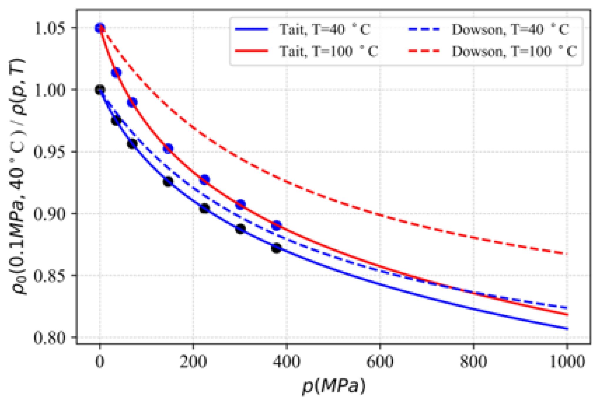
The relative volume has also been plotted for Tait and Dowson equations of state in Figure 2. The data is limited to $400 \mathrm{MPa}$ pressure, whereas the deviation becomes larger at higher pressure, which can be considered the difference in the extrapolation of data using Tait and Dowson equations. In the Dowson EoS, the temperature dependence has been accounted for by multiplying a linear lubricant temperature function with the original model, such that the density of the lubricant can be expressed as the product of two separate density functions: ${\rho }_{Dowson}\left(p,T\right)={\rho }_1\left(p\right)\times {\rho }_2\left(T\right)$. Although this shows correct behaviour at ambient pressure, the influence of temperature at higher pressure has not been taken into account properly. A better fit could be obtained if the constants in Equation (27) depend on temperature. However, such an approach is typically not followed in the literature. Hence, this motivates our choice to use the proposed constants of Dowson as commonly used in the literature.

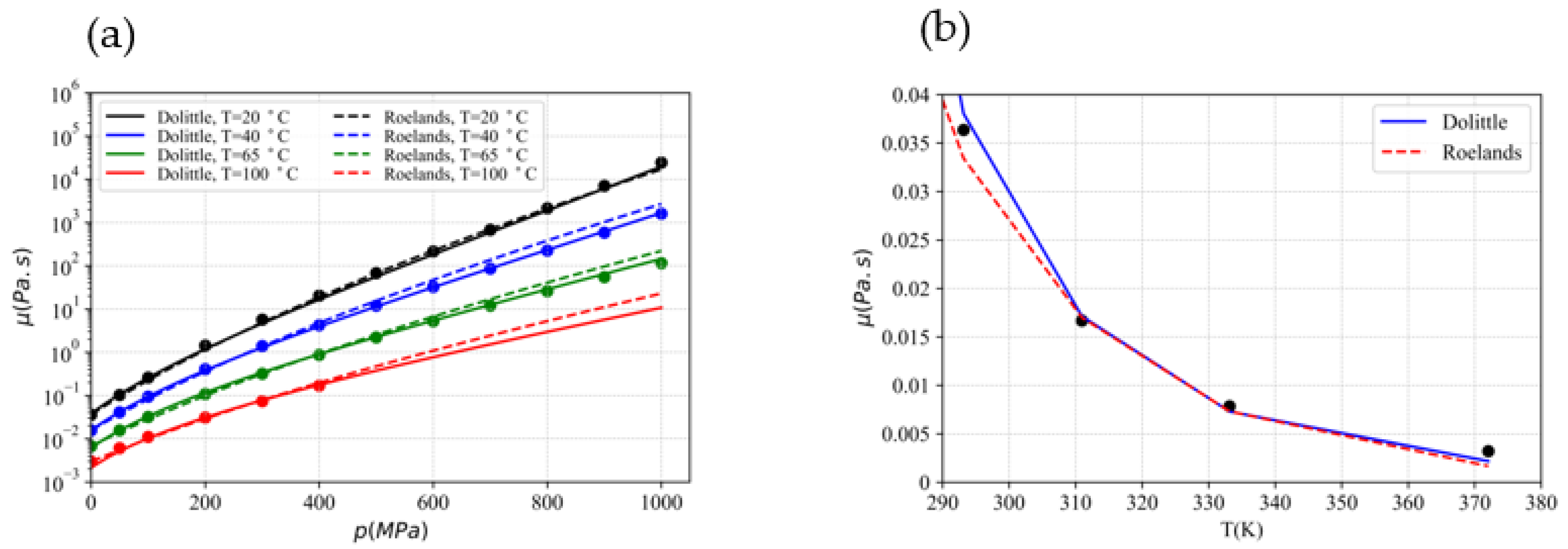
The viscosity is plotted against the pressure for four different temperatures at a zero shear rate in Figure 3a. The point data are experimental data presented in [5,43] for Squalane. A deviation between the predicted Newtonian viscosity by the Roelands–Houpert and Doolittle models can be identified as the pressure and temperature increase. This deviation can be related to the pressure and temperature dependencies of viscosity, $\alpha$ and $\beta$ (please see Equations (28)–(31)). Note that $\alpha$ and $\beta$ are assumed constants and their values have been tuned for each temperature according to the available measured coefficient in [41] to obtain the best-fit curve. It is worth noting that, according to experimental measurement, $\beta$ decreases with an increase in temperature and pressure, whereas $\alpha$ is decreased with temperature and increases with pressure.

Typically, $\alpha$ and β are determined according to the temperature of the lubricant at the inlet. However, the lubricant temperature can go significantly higher than the inlet value, implying that the fixed values of α and β are not consistent anymore in the contact. As a result, considering constant values for the pressure and temperature dependency of viscosity can affect the accuracy of the Roelands Newtonian model. For example, assuming an inlet temperature of $313\mathrm{K}$, using a constant value for $\beta$ according to this temperature leads to a lower viscosity value for lubricant temperature above $313\mathrm{K}$ than what is presented in Figure 3a.

It is worth emphasizing once again that the authors follow the common approach in the literature, in which $\alpha$ and $\beta$ are constant and selected based on the inlet condition, whereas the authors are aware that these parameters should be temperature- and pressure- dependent.

Additionally, the temperature dependency of viscosity at atmospheric pressure is shown in Figure 3b, in which both models have a slight deviation in comparison to experimental data. This plot contains a limited amount of data, whereas more data on a broader temperature range would be beneficial to evaluate the Doolittle versus Roelands models.

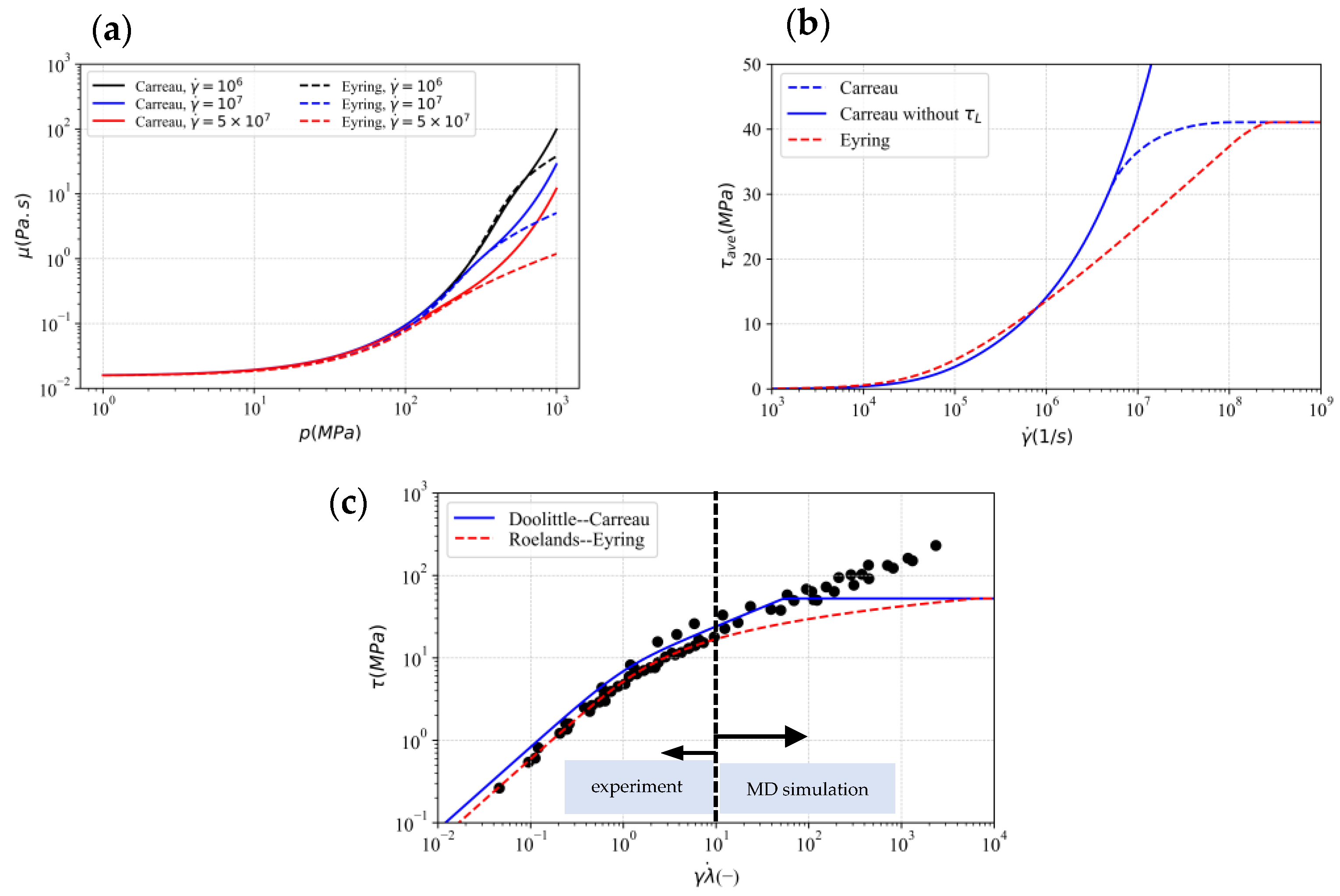
Finally, the shear dependency of viscosity models is illustrated in Figure 4a. The viscosity at different shear rates is plotted against the pressure. In brief, the deviation between models becomes more significant as the pressure and shear rate increase, and the Carreau model predicts a higher viscosity value than Eyring. Figure 4b displays the mean shear stress as a function of the shear rate for a maximum contact pressure of $0.7 \mathrm{GPa}$ and an inlet temperature of $313 \mathrm{K}$. The mean shear stress profiles of the Eyring and Carreau models are clearly different at high shear rates. The mean shear stress, predicted by the Carreau model, requires limiting shear stress in order to prevent a continuous rise of the shear stress. Additionally, the limiting shear stress has been incorporated into the Eyring model. The master curve is also presented in Figure 4c, indicating a deviation between Eyring and Carreau shear thinning models in the log–log scale. The point data for $\dot{\gamma }\lambda <10$ are experimental data [7], and the other part of data are extracted from non-equilibrium Molecular Dynamic (MD) simulations [44,45]. The MD results at high shear stress cannot be perfectly fitted by any of these models. Furthermore, MD simulation cannot describe the limiting shear stress. Even so, Carreau and Eyring can be compared with the master curve.

4. Results

In the following sections, the simulation results obtained with both constitutive groups will be compared in detail. According to what we previously explained, the parameters for the density and viscosity models are set based on the inlet temperature ($T=313 \mathrm{K}$). The lubrication of steel materials exposed to an external load of 100$\mathrm{kN}/\mathrm{m}$is investigated. The equivalent radius of curvature is $10 \mathrm{mm}$, and the entrainment velocity of $2.5 \mathrm{m}/\mathrm{s}$ with a slide-to-roll ratio of SRR = 1, except for the cases mentioned in the text.

Note that the $\mathrm{SRR}$ is defined as

$$SRR=\frac{u_1-u_2}{\frac{u_1+u_2}{2}}$$

(37)

where $u_1$ and $u_2$ are the speeds of the rigid plate and equivalent roller, respectively. Note that the speed of the rigid plate is always equal to or greater than the equivalent roller. In the case of $\mathrm{SRR}=2$, the equivalent body is stationary.

Additionally, CoF is calculated by considering the sum of shear forces acting on the rigid plate in the flow or tangential direction. Accordingly, the CoF calculated in this study is as follows:

$$CoF=\frac{f_{\tau }}{f}=\frac{{\displaystyle \int }\overrightarrow{{\tau }_w}.\overrightarrow{e_t}dA}{{\displaystyle \int }p.\overrightarrow{e_n}dA}$$

(38)

4.1. Shear Rate Modelling Effects

To investigate the role of the shear thinning model, numerical simulations are performed for different SRRs varying from 0 to 2. The film thickness, shear rate, and temperature field will be analyzed to provide more insight into the sensitivity of the numerical solution to the constitutive laws. As the sliding velocity increases, the shear stress and frictional forces rise, resulting in a more pronounced shear thinning and viscosity reduction. At the same time, the increased shear stresses lead to a reduction in shear heating, which further decreases the viscosity. Obviously, because of viscosity reduction, the film thickness has to decrease, as shown in Figure 5. It can be seen that the TDC group predicts a thicker film, which can be attributed to the higher viscosity value calculated by the combination of the Doolittle and Carreau models. The central film thickness deviates by up to 7% under the investigated conditions. Here, the central film thickness is reported at $x=0$, although there is some variation in film thickness around this point.

Furthermore, a slight variation in film thickness is noted for the case of $\mathrm{SRR}=0$, where a constant film thickness is expected due to the surfaces entraining the lubricant at the same speed into the contact region. Two possible reasons could account for this variation: firstly, the EHL pressure profile itself is not symmetrical around the centre of contact, which could contribute to the observed variation. Secondly, using an equivalent body and half-space approach in this study can introduce further deviations from the idealized symmetrical geometry, which could also contribute to the variation in film thickness.

Figure 6 shows the viscosity profile over the equivalent roller only at SRR = 0 for the sake of simplicity. This study found that the Roelands and Doolittle models show different viscosity variations at the inlet region. Furthermore, while the DRE group has a higher viscosity at the contact point, it has a lower viscosity value at the inlet. It might seem less important at first glance, but it can also have a significant impact on the central film thickness. The lubricant film is thinner for DRE, despite its higher viscosity at the centre of contact than for TDC, because the inlet viscosity is lower. In other words, if the reciprocal asymptotic isoviscous pressure coefficient (${\alpha }^{\ast }=\frac{1}{{{\displaystyle \int }}_0^{\infty } \frac{\mu \left(p=0\right)}{\mu \left(p\right)}dp}$) is calculated for the Roelands and Doolittle models [46], the former has $16.4 {\mathrm{GPa}}^{-1}$ and the latter has $17.8 {\mathrm{GPa}}^{-1}$. This implies that using the Roelands model results in a thinner film.

Additionally, from Figure 5a, one can observe small differences in the contact width, with the DRE group predicting a slightly wider contact. A similar trend was also observed in [17], although not discussed in detail. The study results indicate that the low-pressure behaviour of the viscosity model is a contributing factor to the aforementioned phenomenon. Specifically, the pressure–viscosity dependency at the low pressure region (inlet region) can have a significant impact on both the central film thickness and the contact width.

In Figure 7, temperature distributions are shown on the roller surface as a function of the SRR for both TDC (dash lines) and DRE (solid lines) constitutive model groups. It is clear that the temperature distribution is noticeably affected by the particular choice of the constitutive model group. Although the trend of changes is similar, the temperature is predicted to be higher by the TDC group. At low SRR ($0<\mathrm{SRR}<0.2$), temperature effects are limited; therefore, the differences between the results of both groups are attributed to the differences in the approximations of the piezoviscous and shear behaviour at low shear rates. At higher shear rates ($\mathrm{SRR}>0.2$), deviations between models are not only due to shear thinning models but also due to the temperature dependency of Newtonian viscosity models. Since constant pressure/temperature–viscosity coefficients have been used for the Roelands model, the obtained viscosity will be underestimated as the temperature and pressure rise up in the contact region.

The lubricant temperature rise depends on shear stress and velocity difference of surfaces ($\overline{\tau }.\Delta u$) [47]. A significant increase in shear stress is observed when SRR is less than 0.2, and then there is no noticeable change (a discussion of this will take place later). Accordingly, as shown in Figure 7d, temperature rise initially increases non-linearly but then almost linearly. Regarding the comparison between the two groups, the maximum temperature of the lubricant varies by as much as $28\%$.

Figure 8 presents viscosity, shear rate, and shear stress profiles as a function of SRR. The viscosity varies significantly across the lubricant film in the DRE group, which can also influence the flow pattern (velocity vectors). Moreover, the shear rate reveals some minor deviations, especially in the middle of the lubricant film. As the SRR increases, the deviations in shear rate, reported as an average on the centre of contact, become larger. It appears that DRE predicts a higher shear rate. Even though the deviations can be traced back to the viscosity models themselves, the higher shear rates observed in the DRE group will also amplify the film thickness reduction, resulting in a further increase in the shear rate. Thus, lubricant behaviour and contact conditions are intimately related.

The shear stress and viscosity are predicted to be lower by the DRE group under the investigated condition. According to Figure 4b, the Eyring model predicts a significantly lower mean shear stress, which can also be observed in the numerical results of Figure 8f. The lower estimated viscosity and mean shear stress by the Eyring model at high pressures and shear rates can also describe the thinner film thickness for the DRE solution of the TEHL contacts.

Figure 9 illustrates the average viscosity of the contact region. The high viscosity value due to the piezoviscous effects is reduced by two different effects: thermal and shear thinning. In addition to the non-Newtonian viscosity ($\mu \left(p,T,\dot{\gamma }\right)$), two other viscosity values have been presented: Newtonian, temperature-dependent viscosity ($\mu \left(p,T,\dot{\gamma }=0\right)$), and iso-thermal non-Newtonian viscosity ($\mu \left(p,T=T_0,\dot{\gamma }\right)$). The former indicates how temperature can reduce viscosity, whereas the latter shows the contribution of shear rate in viscosity reduction. By comparing these curves, we can gain insight into how thermal effects and shear thinning compete for viscosity reduction. Note that the aforementioned viscosity values have been calculated with obtained pressure, temperature, and shear rate fields from the TEHL solution performed before for non-Newtonian fluids, including thermal effects. Hence, isothermal calculation and TEHL simulations for non-Newtonian fluid have not been conducted. It has been observed that $\mu \left(p,T=T_0,\dot{\gamma }\right)$ decreases sharply and further than $\mu \left(p,T,\dot{\gamma }=0\right)$ for approximately $\mathrm{SRR}<1.5$, implying that the shear thinning contributes further to the viscosity reduction in this range of SRR. It appears that these contributions increase as SRR increases, and they are comparable at higher SRRs ($\mathrm{SRR}>1.5$). When comparing the two well-known sets of constitutive equations, the TDC group calculates up to $36\%$ higher average Newtonian viscosity ($\mu \left(p,T,\dot{\gamma }=0\right)$) as well as up to 26% higher average non-Newtonian viscosity under an isothermal condition ($\mu \left(p,T=T_0,\dot{\gamma }\right)$). Consequently, the average non-Newtonian viscosity differs by $27\%$.

Figure 10 compares the CoF for both previously mentioned models. At $\mathrm{SRR}<0.2$, the DRE group predicts slightly a higher friction, while it has a $20 \%$ lower value for higher SRR. The reported deviations in viscosity directly affect the calculation of shear forces and coefficients of friction. As a result, there is a greater deviation in CoF than in film thickness.

4.2. Piezoviscous Modelling Effects

Besides shear dependency, the piezoviscous effect can meaningfully impact the TEHL calculation. The viscosity varies nearly exponentially with pressure, and it increases to a very high value of the order of magnitude of $\mathrm{Pa}.\mathrm{s}$ when the contact pressure is in the order of $\mathrm{GPa}$. Because of the higher pressure gradients in the contact in case of larger pressure–viscosity coefficients, higher shear rates are induced, promoting shear thinning indirectly. Figure 11 shows the average viscosity in the contact as a function of the load for an $\mathrm{SRR}=1$. In order to evaluate the contribution of pressure, temperature, and shear rate to the calculated viscosity, the latter has been decomposed into three contributions, in analogy with the dual decomposition of viscosity in Figure 9. The piezoviscous effect is studied by evaluating viscosity with constant temperature and a zero shear rate denoted as $\mu \left(p,T=T_0,\dot{\gamma }=0\right)$. Evaluating these terms indicates that, except for piezoviscous effects, each contribution is given a higher value when the Doolittle and Carreau models are combined. Hence, a higher non-Newtonian value is calculated under a thermal condition for TDC. Roelands estimates piezoviscous effects $37\%$ higher than Doolittle at a load of $100\mathrm{kN}/\mathrm{m}$, and the deviation between them increases up to $60\%$ at a load of $200\mathrm{kN}/\mathrm{m}$. However, when the temperature effect is taken into account, Roelands predicts almost a $26\%$ lower average viscosity value. Finally, using the DRE group shows up to a $33\%$ deviation in comparison to the TDC group.

In Figure 12, the central film thickness has been plotted for a load varying from $100\mathrm{kN}/\mathrm{m}$ to $200\mathrm{kN}/\mathrm{m}$. As the load increases, the film thickness becomes thinner, and a further shear heating and higher contact temperature are expected. Although the overall trend and shape of the contact are very similar, quantitative deviations between the TEHL solution using TDC and DRE groups are evident. The TDC predicts a higher viscosity value at the inlet and contact region, leading to an approximately $8\%$ thicker film for the TEHL solution using this group under an external load of $140\mathrm{kN}/\mathrm{m}$. The deviation in central film thickness can rise up to $10\%$ at a load of $200\mathrm{kN}/\mathrm{m}$. According to Figure 3a, the Roelands model should predict a higher viscosity value at $40{}^{\mathrm{o}}\mathrm{C}$, while the DRE group has a lower viscosity value, as shown in Figure 11a. This is mainly because of temperature–viscosity dependency. The temperature can increase up to $80{}^{\mathrm{o}}\mathrm{C}$ under investigated condition, and the Roelands model then predicts a lower viscosity value. These deviations can be reduced by including temperature and pressure effects on the pressure/temperature–viscosity coefficients in the Roelands viscosity model. In brief, the deviation between Doolittle and Roelands models becomes more prominent at higher temperatures, which is more evident at high loads.

Figure 13 illustrates the temperature profile on the roller surface for three chosen loads for the TEHL solution using TDC (dash lines) and DRE (solid lines) groups. The temperature profiles show a wide deviation not only at the contact region but also at the outlet region. In studied cases, the temperature is higher when using the TDC group for the TEHL problem. The TDC calculates the maximum lubricant temperature to be up to 38% higher than DRE. This higher temperature is explained by higher predicted viscosity at surfaces and the contact region. Although shear heating is by far the most dominant mechanism for temperature variation, the compression work of the liquid also has a minor role in temperature variation [9]. Evaluating numerical results indicates that both shear heating and compression work are also higher in the TDC group because of the higher calculated density and viscosity of the lubricant.

On the other hand, in both groups, the maximum shear stress is not increased as the load rises from $140$kN/m to $180$kN/m. Similarly, although the viscosity continuously increases with load, the shear forces and CoF are reduced for $f>140 \mathrm{kN}/\mathrm{m},$ as shown in Figure 14. The numerical results have been investigated carefully to find the main reason for the observed variation in a more elaborate way. It has been concluded that the drop in CoF is because of changes in the shear rate at the walls. The shear rate at the equivalent roller surface is presented in Figure 15. It becomes evident that the shear rate has a reduction as the load increases from $140 \mathrm{kN}/\mathrm{m}$ to $200 \mathrm{kN}/\mathrm{m}$. In conclusion, the flow pattern and shear forces are influenced by higher loads, leading to a change in the CoF trend for TEHL line contacts. It should be noted that if the load increases further, the lubrication regime can be shifted to the mixed lubrication region, and the CoF should increase because of the asperities’ contact.

In Figure 14b, the CoF curves for both groups show similar variations. Quantitative differences do exist, however. The numerical results reveal up to 31% deviation in this variable. The CoF in the TDC group is estimated to be higher due to the deviations in lubricant properties previously discussed.

5. Conclusions

In this paper, the authors compared two groups of well-known constitutive models, commonly used together, in terms of film thickness, lubricant temperature, and traction curve under different operating conditions. The first group included the Dowson density model and Roelands and Eyring viscosity models. The second group incorporated the Tait model for density along with the Doolittle and Carreau models for viscosity. To avoid the effects of lubricant property averaging, the CFD-FSI approach was employed. A homogeneous equilibrium model was employed to account for cavitation, as well as a linear elastic solver and a heat conduction equation to describe material deformation and temperature in solid materials. The deviations in TEHL solution using these sets of constitutive equations for Squalane lubricant were quantified for a wide range of operating conditions. The research findings led to the following main conclusions:

• Using a constant viscosity–temperature coefficient as typically performed in the literature, the Roelands model is observed to underestimate the temperature effects on EHL parameters.
• It has been observed that shear thinning has a more noticeable impact on viscosity calculation than the temperature in the cases studied. Comparing TDC and DRE revealed that the Eyring model calculates a lower viscosity value than the Carreau model. This can be attributed to the fundamental nature of the Eyring equation. The lower viscosity value, calculated by combining the Roelands and Eyring models, resulted in a thinner film, lower lubricant temperature, and lower CoF for TEHL contacts.
• The results indicated that depending on the constitutive model used, the central film thickness could change by up to $10\%$, the CoF can vary up to $31\%$, and the maximum lubricant temperature can differ by up to $38\%$ when the load is $100\mathrm{kN}/\mathrm{m}$ to $200\mathrm{kN}/\mathrm{m}$ and the SRR is between $0$ and $2$.
• As lubricant temperature and CoF are directly linked to viscosity, the observed deviation in viscosity can have a substantial impact on them. Consequently, deviations in the CoF and temperature are more significant than those in, e.g., the central film thickness, as the latter is governed by the viscosity rise in the low-pressure inlet region rather than that in the centre of the contact.

References

1. Dowson, D.; Higginson, G.R. Elasto-Hydrodynamic Lubrication: International Series on Materials Science and Technology; Elsevier: Amsterdam, The Netherlands, 2014; ISBN 1483181898. [Google Scholar]
2. Macdonald, J.R. Some Simple Isothermal Equations of State. Rev. Mod. Phys. 1966, 38, 669. [Google Scholar] [CrossRef]
3. Roelands, C.J.A.; Vlugter, J.C.; Waterman, H.I. The Viscosity-Temperature-Pressure Relationship of Lubricating Oils and Its Correlation With Chemical Constitution. J. Basic Eng. 1963, 85, 601–607. [Google Scholar] [CrossRef]
4. Doolittle, A.K. Studies in Newtonian Flow. II. Depend. Viscosity Liq. Free-Space. J. Appl. Phys. 1951, 22, 1471–1475. [Google Scholar]
5. Bair, S. Reference Liquids for Quantitative Elastohydrodynamics: Selection and Rheological Characterization. Tribol. Lett. 2006, 22, 197–206. [Google Scholar] [CrossRef]
6. Bair, S. Actual Eyring Models for Thixotropy and Shear-Thinning: Experimental Validation and Application to EHD. J. Tribol. 2004, 126, 728–732. [Google Scholar] [CrossRef]
7. Bair, S.S. High Pressure Rheology for Quantitative Elastohydrodynamics; Elsevier: Amsterdam, The Netherlands, 2019; ISBN 0128163100. [Google Scholar]
8. Johnson, K.L.; Tevaarwerk, J.L. Shear Behaviour of Elastohydrodynamic Oil Films. Proc. R. Soc. Lond. A Math. Phys. Sci. 1977, 356, 215–236. [Google Scholar]
9. Habchi, W.; Vergne, P. On the Compressive Heating/Cooling Mechanism in Thermal Elastohydrodynamic Lubricated Contacts. Tribol. Int. 2015, 88, 143–152. [Google Scholar] [CrossRef]
10. Hultqvist, T.; Vrcek, A.; Marklund, P.; Prakash, B.; Larsson, R. Transient Analysis of Surface Roughness Features in Thermal Elastohydrodynamic Contacts. Tribol. Int. 2020, 141, 105915. [Google Scholar] [CrossRef]
11. Kumar, P.; Khonsari, M.M. Traction in EHL Line Contacts Using Free-Volume Pressure-Viscosity Relationship With Thermal and Shear-Thinning Effects. J. Tribol. 2008, 131. [Google Scholar] [CrossRef]
12. Conry, T.F. Thermal Effects on Traction in EHD Lubrication. J. Lubr. Technol. 1981, 103, 533–538. [Google Scholar] [CrossRef]
13. Bair, S. A Traction (Friction) Curve Is Not a Flow Curve. Lubricants 2022, 10, 221. [Google Scholar] [CrossRef]
14. Spikes, H.; Jie, Z. History, Origins and Prediction of Elastohydrodynamic Friction. Tribol. Lett. 2014, 56, 1–25. [Google Scholar] [CrossRef] [Green Version]
15. Bair, S.; Vergne, P.; Kumar, P.; Poll, G.; Krupka, I.; Hartl, M.; Habchi, W.; Larsson, R. Comment on “History, Origins and Prediction of Elastohydrodynamic Friction” by Spikes and Jie. Tribol. Lett. 2015, 58, 16. [Google Scholar] [CrossRef]
16. Kumar, P.; Khonsari, M.M. On the Role of Lubricant Rheology and Piezo-Viscous Properties in Line and Point Contact EHL. Tribol. Int. 2009, 42, 1522–1530. [Google Scholar] [CrossRef]
17. Tošić, M.; Larsson, R.; Jovanović, J.; Lohner, T.; Björling, M.; Stahl, K. A Computational Fluid Dynamics Study on Shearing Mechanisms in Thermal Elastohydrodynamic Line Contacts. Lubricants 2019, 7, 69. [Google Scholar] [CrossRef] [Green Version]
18. Bair, S.; Yamaguchi, T. The Equation of State and the Temperature, Pressure, and Shear Dependence of Viscosity for a Highly Viscous Reference Liquid, Dipentaerythritol Hexaisononanoate. J. Tribol. 2017, 139, 011801. [Google Scholar] [CrossRef]
19. Bair, S.; Mary, C.; Bouscharain, N.; Vergne, P. An Improved Yasutomi Correlation for Viscosity at High Pressure. Proc. Inst. Mech. Eng. Part J J. Eng. Tribol. 2013, 227, 1056–1060. [Google Scholar] [CrossRef]
20. Bair, S.; Liu, Y.; Wang, Q.J. The Pressure-Viscosity Coefficient for Newtonian EHL Film Thickness With General Piezoviscous Response. J. Tribol. 2006, 128, 624–631. [Google Scholar] [CrossRef]
21. Bair, S.; Martinie, L.; Vergne, P. Classical EHL versus Quantitative EHL: A Perspective Part II—Super-Arrhenius Piezoviscosity, an Essential Component of Elastohydrodynamic Friction Missing from Classical EHL. Tribol. Lett. 2016, 63, 37. [Google Scholar] [CrossRef] [Green Version]
22. Habchi, W.; Vergne, P.; Bair, S.; Andersson, O.; Eyheramendy, D.; Morales-Espejel, G.E. Influence of Pressure and Temperature Dependence of Thermal Properties of a Lubricant on the Behaviour of Circular TEHD Contacts. Tribol. Int. 2010, 43, 1842–1850. [Google Scholar] [CrossRef]
23. Habchi, W.; Bair, S. The Role of the Thermal Conductivity of Steel in Quantitative Elastohydrodynamic Friction. Tribol. Int. 2020, 142, 105970. [Google Scholar] [CrossRef]
24. Habchi, W.; Bair, S. Quantitative Compressibility Effects in Thermal Elastohydrodynamic Circular Contacts. J. Tribol. 2012, 135, 011502. [Google Scholar] [CrossRef]
25. Bruyere, V.; Fillot, N.; Morales-Espejel, G.E.; Vergne, P. Computational Fluid Dynamics and Full Elasticity Model for Sliding Line Thermal Elastohydrodynamic Contacts. Tribol. Int. 2012, 46, 3–13. [Google Scholar] [CrossRef]
26. Almqvist, T.; Larsson, R. The Navier–Stokes Approach for Thermal EHL Line Contact Solutions. Tribol. Int. 2002, 35, 163–170. [Google Scholar] [CrossRef]
27. Hartinger, M.; Dumont, M.-L.; Ioannides, S.; Gosman, D.; Spikes, H. CFD Modeling of a Thermal and Shear-Thinning Elastohydrodynamic Line Contact. J. Tribol. 2008, 130, 41503. [Google Scholar] [CrossRef]
28. Hartinger, M.; Reddyhoff, T. CFD Modeling Compared to Temperature and Friction Measurements of an EHL Line Contact. Tribol. Int. 2018, 126, 144–152. [Google Scholar] [CrossRef]
29. Hajishafiee, A.; Kadiric, A.; Ioannides, S.; Dini, D. A Coupled Finite-Volume CFD Solver for Two-Dimensional Elasto-Hydrodynamic Lubrication Problems with Particular Application to Rolling Element Bearings. Tribol. Int. 2017, 109, 258–273. [Google Scholar] [CrossRef] [Green Version]
30. Scurria, L.; Tamarozzi, T.; Voronkov, O.; Fauconnier, D. Quantitative Analysis of Reynolds and Navier–Stokes Based Modeling Approaches for Isothermal Newtonian Elastohydrodynamic Lubrication. J. Tribol. 2021, 143, 121601. [Google Scholar] [CrossRef]
31. Hao, L.; Meng, Y. Comparisons of TEHL Simulations of Newtonian Fluids in Line Contacts between the 3D FEM and the Reynolds Equation–Based Approaches*. Tribol. Trans. 2016, 59, 641–654. [Google Scholar] [CrossRef]
32. Weller, H.; Nordin, N. Modelling Injector Flow Including Cavitation Effects for Diesel Applications. In Proceedings of the ASME/JSME 2007 5th Joint Fluids Engineering Conference, San Diego, CA, USA, 30 July 2007; American Society of Mechanical Engineers Digital Collection: New York City, NY, USA, 2007; pp. 465–474. [Google Scholar]
33. Hartinger, M. CFD Modelling of Elastohydrodynamic Lubrication. Ph.D. Thesis, Imperial College London, London, UK, 2007. Available online: https://ethos.bl.uk/OrderDetails.do?uin=uk.bl.ethos.444143 (accessed on 1 March 2023).
34. Hajishafiee, A. Finite-Volume CFD Modelling of Fluid-Solid Interaction in EHL Contacts; Imperial College London: London, UK, 2013; Volume C. [Google Scholar]
35. Kim, H.J.; Ehret, P.; Dowson, D.; Taylor, C.M. Thermal Elastohydrodynamic Analysis of Circular Contacts Part 2: Non-Newtonian Model. Proc. Inst. Mech. Eng. Part J J. Eng. Tribol. 2001, 215, 353–362. [Google Scholar] [CrossRef]
36. Kim, H.J.; Ehret, P.; Dowson, D.; Taylor, C.M. Thermal Elastohydrodynamic Analysis of Circular Contacts Part 1: Newtonian Model. Proc. Inst. Mech. Eng. Part J J. Eng. Tribol. 2001, 215, 339–352. [Google Scholar] [CrossRef]
37. Cardiff, P.; Karač, A.; De Jaeger, P.; Jasak, H.; Nagy, J.; Ivanković, A.; Tuković, Ž. An Open-Source Finite Volume Toolbox for Solid Mechanics and Fluid-Solid Interaction Simulations. arXiv 2018, arXiv:1808.10736. [Google Scholar]
38. Habchi, W. A Full-System Finite Element Approach to Elastohydrodynamic Lubrication Problems: Application to Ultra-Low-Viscosity Fluids; Univ. Lyon. Fr.: Lyon, France, 2008. [Google Scholar]
39. Björling, M.; Habchi, W.; Bair, S.; Larsson, R.; Marklund, P. Friction Reduction in Elastohydrodynamic Contacts by Thin-Layer Thermal Insulation. Tribol. Lett. 2014, 53, 477–486. [Google Scholar] [CrossRef] [Green Version]
40. Hultqvist, T.; Vrček, A.; Marklund, P.; Larsson, R. On Waviness and Two-Sided Surface Features in Thermal Elastohydrodynamically Lubricated Line Contacts. Lubricants 2020, 8, 64. [Google Scholar] [CrossRef]
41. Pensado, A.S.; Comuñas, M.J.P.; Lugo, L.; Fernández, J. High-Pressure Characterization of Dynamic Viscosity and Derived Properties for Squalane and Two Pentaerythritol Ester Lubricants: Pentaerythritol Tetra-2-Ethylhexanoate and Pentaerythritol Tetranonanoate. Ind. Eng. Chem. Res. 2006, 45, 2394–2404. [Google Scholar] [CrossRef]
42. Bair, S. The High Pressure Rheology of Some Simple Model Hydrocarbons. Proc. Inst. Mech. Eng. Part J J. Eng. Tribol. 2002, 216, 139–149. [Google Scholar] [CrossRef]
43. Comuñas, M.J.P.; Paredes, X.; Gaciño, F.M.; Fernández, J.; Bazile, J.-P.; Boned, C.; Daridon, J.-L.; Galliero, G.; Pauly, J.; Harris, K.R. Viscosity Measurements for Squalane at High Pressures to 350 MPa from T=(293.15 to 363.15) K. J. Chem. Thermodyn. 2014, 69, 201–208. [Google Scholar] [CrossRef]
44. Gupta, S.A.; Cochran, H.D.; Cummings, P.T. Shear Behavior of Squalane and Tetracosane under Extreme Confinement. III Eff. Confin. Viscosity J. Chem. Phys. 1997, 107, 10335–10343. [Google Scholar]
45. Moore, J.D.; Cui, S.T.; Cummings, P.T.; Cochran, H.D. Lubricant Characterization by Molecular Simulation. Am. Inst. Chem. Eng. AIChE J. 1997, 43, 3260. [Google Scholar] [CrossRef]
46. Spikes, H. Basics of EHL for Practical Application. Lubr. Sci. 2015, 27, 45–67. [Google Scholar] [CrossRef] [Green Version]
47. Archard, J.F. The Temperature of Rubbing Surfaces. Wear 1959, 2, 438–455. [Google Scholar] [CrossRef]
Figure 1. A schematic view of the 2D geometry.
Lubricants 11 00151 g001
Figure 2. Density ratio against pressure at two different temperatures.
Lubricants 11 00151 g002
Figure 3. (a) Viscosity against pressure for the different temperatures at zero shear rate, (b) viscosity at ambient pressure and zero shear rates for different temperatures.
Lubricants 11 00151 g003
Figure 4. (a) Viscosity against pressure for the different shear rates at T = 313   K , (b) mean shear stress against shear rate for a maximum contact pressure of 0.7   GPa and T = 313   K , (c) master flow curve at a maximum contact pressure of 0.7   GPa and inlet temperature of T = 313   K . On the x axis,   λ = μ N e w t o n i a n / G represents the rotational relaxation time.
Lubricants 11 00151 g004
Figure 5. (a) Film thickness profile and (b) central film thickness as a function of SRR.
Lubricants 11 00151 g005
Figure 6. Viscosity profile on roller surface for SRR = 0 .
Lubricants 11 00151 g006
Figure 7. (a) Temperature distribution for (a) TDC and (b) DRE groups for SRR = 1 , (c) temperature profile over equivalent roller surface, (d) maximum temperature rise as a function of SRR.
Lubricants 11 00151 g007
Figure 8. Viscosity distribution for (a) TDC and (b) DRE, shear rate distribution for (c) TDC and (d) DRE group for SRR = 1 , (e) average shear rate at the centre of contact, (f) shear stress profile over equivalent roller surface as a function of SRR.
Lubricants 11 00151 g008
Figure 9. (a) Average viscosity at the contact as a function of SRR, (b) average viscosity in the thermal condition with a zero shear rate (Newtonian viscosity), and average viscosity in the iso-thermal condition as a function of SRR.
Lubricants 11 00151 g009
Figure 10. CoF as a function of SRR.
Lubricants 11 00151 g010
Figure 11. Average non-Newtonian viscosity in thermal conditions and iso-thermal conditions, Newtonian viscosity in thermal conditions and iso-thermal conditions for (a) TDC and (b) DRE as a function of load at SRR = 1 .
Lubricants 11 00151 g011
Figure 12. (a) Film thickness profile, (b) central film thickness, as a function of load at SRR = 1 .
Lubricants 11 00151 g012
Figure 13. (a) Temperature profile over equivalent roller surface, (b) maximum temperature rise as a function of load at SRR = 1 .
Lubricants 11 00151 g013
Figure 14. (a) Shear stress profile over equivalent roller surface, (b) CoF as a function of load at SRR = 1 .
Lubricants 11 00151 g014
Figure 15. Shear rate on equivalent roller surface as a function of load at SRR = 1 for (a) TDC group and (b) DRE group.
Lubricants 11 00151 g015