1. Introduction
Many experts in the field of musculoskeletal system biomechanics believe that synovial joints can be classified as “smart” friction pairs, which, in a healthy human body, self-adjust so that they form an optimal tribological structure in relation to the function performed [
1,
2,
3]. This authoritative point of view leads to many questions about the natural organization and practical implementation of the self-adjustment and control processes of the joints’ functioning. In this regard, such branches of science as anatomy, physiology, and biomechanics of joints have a long history and continue to develop. However, up to the present time, there is no complete understanding of the joints’ operation and their adjustment to perform a specific function.
Theoretical and experimental studies of synovial joints and their elements are performed at different levels: chemical, biological, biochemical, biomechanical, etc. As a result, a huge amount of information has been accumulated, which makes it possible to predict various events that accompany the joints’ operation with a certain probability. However, under in vivo conditions, events are often observed that differ greatly from those predicted theoretically. So, for example, up to the present time in natural experiments, it has not possible to obtain the coefficient of friction in the synovial joint as in in vivo conditions; there is no complete understanding the degeneration and restoration processes of articular cartilage, etc. In this regard, to obtain theoretical estimates and solve actual applied problems, phenomenological models of the synovial joints’ functioning are often used. From this point of view, taking into consideration the extremely important role of joints in the implementation of human movements, models of their lubrication are of great interest; a significant contribution to the development of which was made by D. Dowson et al. [
4,
5,
6,
7,
8,
9,
10]. There are also many works by other authors who have paid great attention to this topic of research. At the same time, it should be noted that, despite the hypothetical foundations on which most phenomenological models are built, in most cases they allow us to evaluate tribological processes in the joints and find their optimal parameters with sufficient accuracy for practice. To a large extent, this is facilitated by a new understanding of the biological lubrication processes of synovial joints at the molecular level, of which much progress has been made to date [
11]. In fact, studies of synovial joints at the biochemical level allow us to make fairly reasonable assumptions about the cellular and chemical processes occurring in the elements of the joints under various conditions. Based on these assumptions, approximate biomechanical mathematical models are constructed, in which cellular and chemical processes are indirectly taken into consideration. Thus, it becomes possible to study the biomechanical features of such “smart” friction pairs as synovial joints, using relatively simple models. Paradoxical as it may seem, in practice this approach often leads to better results than in the study of complex models with many heterogeneous parameters, even in cases where we are not talking about the so-called the “curse of dimensionality” effect. Thus, it can be argued that mathematical modeling and in silico studies of synovial joints and their elements are powerful tools used to solve complex applied problems, which has been especially pronounced in recent decades due to the rapid development of computer technology and computing environments. One of these tasks is to determine the optimal conditions for the restoration of articular cartilage (AC) defects with various etiological factors and, above all, at various stages of osteoarthritis.
Osteoarthritis (OA) is a degenerative-dystrophic joint disease caused by degradation of the articular surface cartilage tissue [
12], which, according to World Health Organization experts, is one of the main causes of disability, especially for the elderly [
13]. AC degradation and development of OA can result from trauma, disease, or chronic mechanical stress and is classified into three main types: superficial destruction, in which the extracellular matrix (ECM) of the tissue is damaged; defects in the incomplete thickness of the AC that do not extend to subchondral bone; and full-thickness defects, penetrating deep into the subchondral bone [
14]. Only with superficial destruction can viable cartilage tissue cells cluster together and potentially be capable of independently synthesizing a new ECM. With deep-seated defects of all types, self-healing of AC is practically excluded; therefore, for the purpose of their therapeutic or surgical restoration, a number of strategies have been developed, which in most cases, however, do not guarantee positive results either [
15,
16,
17]. Therefore, the task of developing efficient technologies and methods for repairing AC defects at all stages of OA development is relevant. One of the most significant problems that arises on the way to the creation of such technologies lies in the features of AC as a biological tissue, which are well studied and described in great detail in the literature.
AC is a biological tissue composed of basic chondrocyte cells surrounded by abundant ECM, including water, type II collagen, proteoglycans rich in glycosaminoglycans, and a small amount of non-collagenous proteins and glycoproteins. The most important difference between AC and bone and most other tissue types is the absence of nerves and blood vessels within it. Its main function is to absorb and distribute the external load acting on the joint and provide low friction to facilitate smooth movement in the joint. The AC of the synovial joint is surrounded on one side by the joint fluid produced by the adjacent synovial membrane, and on the other side it borders the subchondral bone plate. When a compressive load is applied to the AC, pressure instantly rises in the ECM, which leads to a relatively slow extrusion of interstitial fluid from it, which overcomes the high frictional resistance due to the low permeability of the medium. After the compressive load is removed, the interstitial fluid flows back into the ECM. This process is explained on the basis of a two-phase AC model represented by a mixture of an ideal interstitial fluid and a poroelastic homogeneous isotropic incompressible matrix [
1]. In the context of this study, such a model plays an important role, since at the same time, it allows us to explain the implementation of various lubrication regimes and the viability of AC cells, which is ensured by the supply of nutrients from the synovial fluid to the tissue. A detailed description of the structure and function of AC can be found in many sources in the literature, for example, in [
18].
Thus, the avascular structure of AC and chondrocyte metabolism determine cartilage homeostasis, which depends mainly on the diffusion into the ECM of nutrients, oxygen, and other regulatory factors from the synovial fluid located in the joint cavity. Nutrients entering the AC through the blood vessels from the subchondral bone are consumed primarily to maintain the viability of young cartilage tissue. Taking into account these features of AC, a number of strategies have been developed aimed at improving the effectiveness of OA treatment and repairing AC defects [
19].
Because chondrocytes located in the ECM are regularly exposed to various kinds of external loads, they respond to them to maintain the function of the joint. Many studies are known, as a result of which it was confirmed that mechanical stimulation of the tissue, causing it to be adequately stressed, can promote chondrogenesis during fetal development or maintain cartilage tissue homeostasis in adults [
20]. At the same time, strong mechanical stress disrupts the metabolic activity of chondrocytes and, consequently, cartilage homeostasis [
21]. Other pathways have also been shown to play a role in the regulation of mechanotransduction in chondrocytes [
22]. Thus, it is possible to potentially increase the regenerative capacity of AC by using mechanical tissue stimulation both in the process of cell culture propagation and preparation of explants in vitro to mimic the natural environment of AC, and at the stage of cell therapy in vivo.
Relatively recently, it has been found that mechanical stress can enhance the chondrogenesis of mesenchymal stem cells (MSCs), which is presumably associated with increased chondrogenic signaling mediated by TGF-β [
22,
23]. In addition, it has been shown that adequate mechanical loading of MSCs increases angiogenic capacity [
24], improves collagen formation, cell viability, and fiber organization in tissue engineering constructs [
25,
26]. The features of MSCs noted above, including their ability to differentiate into chondrocytes, as well as the fact that they are easy to harvest with minimal trauma to the donor site, formed the basis of one of the promising strategies for the OA treatment and the repair of AC defects, called “Articular Stem Cell Implantation Technology” (ASIT). The MSCs required for ASIT implementation are obtained from various autologous tissues, including bone marrow, adipose tissue, and peripheral blood [
27] and, depending on the specific pathology, are either surgically implanted into the defect or injected into the joint. Despite the obvious potential prospects for ASIT, postoperative analysis shows that the effectiveness of this technology according to the International Cartilage Repair Society standards is still not high enough, and it needs to be improved [
28].
Another strategy developed to treat certain symptomatic synovial articular cartilage defects using autologous chondrocytes has been called Autologous Chondrocyte Implantation Technology (ACIT). Usually, its implementation involves three stages [
29,
30,
31]. At the first of these, arthroscopy of the patient’s joint is performed with a sampling of 200–300 m of cartilage, usually from the least loaded area. ECM is enzymatically removed from the harvested tissue and chondrocytes are isolated. At the second stage, these cells are grown in a specialized bioreactor under in vitro conditions until their number is sufficient for implantation into the defect area, which takes approximately 1.0–1.5 months. In recent years, ACIT has been improved, and at this stage, they began to use modern biodegradable scaffolds or hydrogels, which contribute to the accelerated formation of three-dimensional ECM tissue. This modification of ACIT, called “Matrix-Induced Autologous Chondrocyte Implantation Technology” (MACIT), is becoming increasingly popular due to its cost-effectiveness compared to first-generation ACIT, as well as better cell maturation in vitro and better cell growth in vivo [
31]. Finally, at the third stage, the cells grown in the bioreactor are implanted into the defect area, adapt to the new environment, and form a new cartilage. It should be noted that, like ASIT, this technology also needs to be improved.
The strategies described above are in line with the state of the art in regenerative medicine and have only limited success in OA treatment and repairing AC defects. However, the improvement of cellular technologies, the development of new biomaterials for the manufacture of scaffolds, and the use of optimal modes for being regenerated tissue mechanical stimulation can provide a basis for the development of more effective technologies for OA treatment. One of the problems to be solved in this case in the near future is to suppress the activation and proliferation of fibrogenic cells, excessive secretion, and deposition of ECM proteins, which can contribute to the formation of fibrocartilage [
32,
33]. In addition, there is the problem of determining the optimal number of cells recruited to the area of the AC defect in order to prevent the formation of fibrocartilage [
34,
35] and a number of others. Thus, at present, the task of developing new technologies to achieve full AC recovery in the area of the defect, while preventing fibrosis of the hyaline cartilage and promoting hyalinization of the fibrocartilage, is currently relevant [
36]. In recent years, a number of optimistic results have been obtained, indicating the potential possibility of solving it through the parallel use of the regenerative and rehabilitation medicine methods, which led to the creation of a new direction in medical science: regenerative rehabilitation [
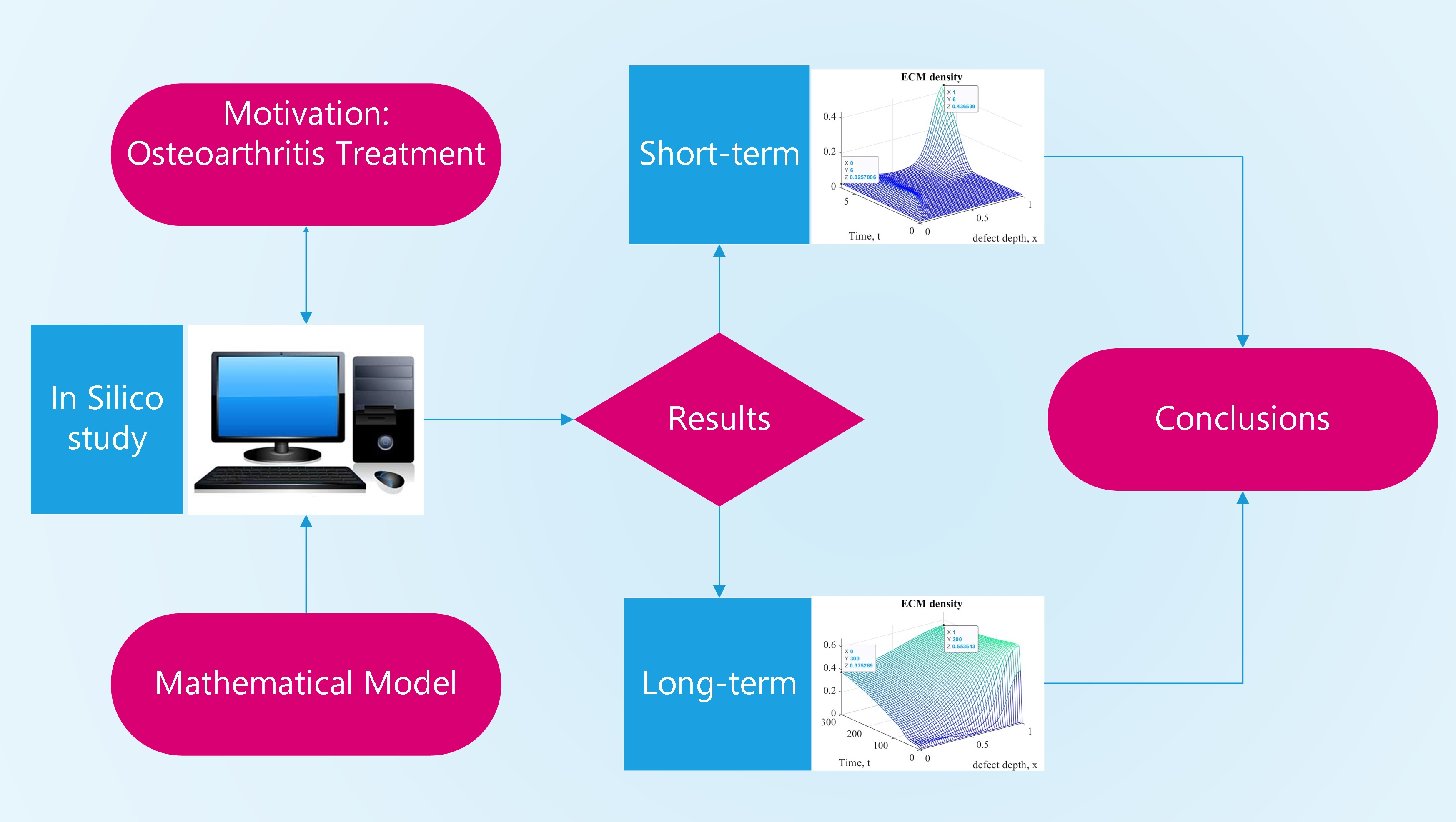
1]. However, for the practical implementation of regenerative and rehabilitation procedures in OA treatment, it is necessary to solve a number of related problems, which are primarily related to the optimization of regenerative and rehabilitation processes without violating their synergistic unity. Such processes obviously depend on many factors, including the biophysical state of the tissue being restored and the characteristics of its interaction with surrounding tissues. The study of these processes under in vivo conditions is limited not only by modern technological means but also by ethical considerations. In this regard, the best approach to studying the process of AC regenerative rehabilitation is to study its mathematical model in silico and compare the obtained results with the results of the tissue restoration experimental studies. The main goal of this work is to predict in silico short-term and long-term results of AC regenerative rehabilitation based on a mathematical model that takes into account the diffusion of cells and nutrients into the defect area during ASIT/ACIT implementation under mechanical stimulation of explants in vivo.
D. Balding and D. McElwain were the first to use a mathematical model of the “diffusion-response” type in 1985 to simulate the dynamics of tumor-induced angiogenesis [
37], modifying the approach previously used by L. Edelstein to describe the growth of fungi [
38]. Somewhat later (in 1990), J. Sherratt and J. Murray developed a model of epidermal wound healing that takes into consideration the interaction between endothelial cells (ECs) and chemoattractant [
39], which assumed that cells randomly move, multiply, and die, while the chemoattractant is produced by cells, diffuses, and undergoes natural decay. The predictions made on the basis of this model were in good agreement with the experimental data, despite the fact that it did not take into account the migration of Ecs up the chemical gradient, and chemotaxis is an important process in wound healing [
40]. In 1993, M. Chaplain and A. Stuart developed a model of the chemotactic response of ECs to tumor angiogenesis factor [
41], and in 1995, H. Byrne and M. Chaplain refined it by including the development of blood vessels in response to tumor angiogenesis factor [
42].
In 1996, M. Chaplain M. and H. Byrne established an important connection between the mathematical simulation of tumor-induced angiogenesis and angiogenesis of wound healing [
43], which contributed to the development of a whole family of mathematical models of angiogenesis in wound healing, among which it is important to note the models developed by G. Pettet et al. [
44,
45]. It is these models that have inspired many authors to study this process in detail ([
46,
47,
48,
49], etc.).
Many mathematical models of bone fracture healing also have a diffusion–response structure. For example, such a model, which takes into consideration the effect of growth factors in fracture healing, was developed by A. Bailo’n-Plaza and M. Van Der Meulen [
50]. There are also mathematical models that simulate the growth of artificial cartilage in vitro [
50,
51,
52,
53], in which, along with cell growth, the consumption of nutrients (mainly oxygen) necessary for their growth and reproduction is considered. One-dimensional diffusion–response models of nutrient transport were developed to predict the profile of oxygen tension in the AC depending on its thickness and cell density, and the parameters used in them, which determine the oxygen concentration gradient in the AC in the direction of the subchondral bone, were experimentally determined and modeled by S. Zhou et al. [
54,
55].
M. Lutianov et al., based on the models developed by L. Olsen et al. [
56] for wound healing and A. Bailo´n-Plaza and M. Van Der Meulen [
50] for fracture healing, developed a mathematical model of AC regeneration after cell therapy, which focused on the production of ECM through migration and proliferation of chondrocytes/MSCs, as well as on the differentiation of MSCs into chondrocytes [
57]. In this model, cell proliferation and differentiation are modulated by available nutrients, and migration, proliferation, cell differentiation, diffusion and nutrient depletion, and ECM synthesis and degradation are modulated and modeled at the defect site both spatially and temporally. In fact, this model made it possible for the first time to evaluate the process of cartilage tissue regeneration under conditions of cell therapy. Later, it was used by K. Campbell et al. to study AC regeneration processes, taking into account the influence of growth factors [
58], and under conditions of cell implantation according to ACIT/ASIT [
59], as well as by V. Popov et al. to assess the effect of mechanical stimulation [
60]. In this paper, this model is taken as the basis for studying the process of AC regenerative rehabilitation with delayed rehabilitation procedures.
2. Materials and Methods
Given the fact that ASIT/ACIT implies the use of MSCs and autologous chondrocytes implanted in the area of the defect in the process of AC regenerative rehabilitation, differential equations of the “diffusion-response” type, simulating changes in their densities (
and
, respectively), are presented in the following form [
57]:
where
is the Laplace operator;
;
are the diffusion coefficients of MSCs and chondrocytes, respectively;
is a concentration of nutrients that provide tissue homeostasis (
are the threshold and critical concentrations, respectively);
are the coefficients that determine proliferation, differentiation and death of MSCs, and
are the coefficients of proliferation and death of chondrocytes, respectively; and
are the Heaviside step functions.
Here and below, we use the designations of the parameters and state variables for the model adopted earlier by K. Campbell et al. in [
58,
59].
It follows from Equation (1) that the change in the defect region is determined by four terms on the right side, which describe the processes of diffusion, proliferation, differentiation, and death of MSCs. At the same time, the increase in cell density depends on the number of MSCs implanted in the defect area and their entry into this area as a result of diffusion from the subchondral bone. If the concentration of nutrients in the defect area is greater than the critical one (), MSCs proliferate, which also leads to an increase in their density. Otherwise, due to a lack of nutrients (), a certain number of MSCs die, which leads to a decrease in their density. In addition, the decrease in occurs due to the fact that, when the threshold density is exceeded, some MSCs differentiate into chondrocytes as a result of commitment.
Formula (2) similarly represents the change in the density of autologous chondrocytes in the area of the defect. Its fundamental difference from Formula (1) is that the differentiation of MSCs leads to a decrease and, at the same time, to an increase in .
Taking into consideration the meaning of the equations’ structure elements (1) and (2), the mathematical model of the change in the concentration of nutrients can be represented as follows:
where
is the coefficient of nutrients diffusion into the defect area from the synovial cavity, and
are the nutrient consumption constants of MSCs and chondrocytes, respectively.
Thus, it is assumed that the nutrients that enter the defect as a result of diffusion through the AC surface are spent on maintaining the viability of MSCs and chondrocytes.
The change in the density of ECM
m, considering the diffusion of its elements through the subchondral plate and secretion by chondrocytes, can be represented by the equation:
given that
, where
is the diffusion coefficient of ECM elements;
is the ECM secretion rate; and
is the maximum ECM density.
Finally, taking into consideration the fact that growth factors play an important role in maintaining the equilibrium state and regeneration of AC, the change in their concentration in the defect area is simulated by the following equations:
where
are the concentrations of growth factors FGF-1 and BMP-2, respectively, and
are the diffusion coefficients, constant secretion, and degradation of growth factors FGF-1 and BMP-2, respectively.
The set of Equations (1)–(6) is a mathematical model of AC regeneration, previously used by K. Campbell et al., under the condition of ASIT/ACIT implementation. However, rehabilitation procedures provided for in regenerative rehabilitation protocols and including mechanical stimulation of the tissue being restored are usually applied with a certain time delay in order to achieve the best results, which, as shown, for example, in [
61], is highly desirable because it allows the maximum effect of tissue restoration to be achieved. Therefore, in the mathematical model of regenerative rehabilitation with the same delay, changes in the parameter values determined by the nature of mechanical stimulation should be taken into consideration.
If we assume that stimulation of the explant populated with chondrogenic cells according to the ASIT/ACIT protocols and placed at the site of a local AC defect begins at time
, then Equations (1) and (2) can be represented as follows:
where
is the Heaviside step function.
Thus, the mathematical model of the regenerative rehabilitation for a local defect in the AC is represented by a system of differential equations in partial derivatives (7), (8) and (3)–(6). In general, it can be used to study state variables that change over time in three-dimensional space. However, due to the fact that the main goal of this research is to assess the cartilage tissue formation at the early and late stages of the regenerative rehabilitation process, it is sufficient to study a one-dimensional model that allows studying the change in state variables only in terms of defect depth h. This limitation is also admissible from a geometric point of view, if the dimensions of the defect (h and b) are small compared to the dimensions of the articular surface, and its curvature in the defect area tends to zero.
The mathematical model studied in this work takes into consideration the use of ASIT/ACIT, which involves the implantation of tissue-engineered constructs into the defect area, including scaffolds seeded with MSCs or chondrocytes. One of the tissue-engineered construct functions is to hold the cells together in order to provide a suitable microenvironment, the proper level of hydration, and, if possible, to further stimulate their proliferation and metabolic activity. Therefore, the scaffold underlying it must meet the above requirements, which is ensured by the proper selection of its structure and material. In particular, such a property of the scaffold as porosity is of particular importance, on which the provision of cells with a medium for diffusion and convection of nutrients depends. With this in mind, it was assumed that the scaffold porosity should be 50–60% with a pore size of 40–50 µm. This, firstly, does not contradict the nutrient diffusion coefficient adopted in numerical experiments [
54], and secondly, it ensures good proliferation of chondrocytes, production of type II collagen and aggrecans, and expression of the MSCs differentiation marker into chondrocytes SOX-9, which is confirmed by experiments [
62]. Thus, in numerical experiments, the initial cartilage porosity in the area of the defect was assumed to be equal to the porosity of the explant (60%) with a pore size of ~40 µm. Subsequently, its change has not been considered under the assumption that in the long term the scaffold biodegrades, and, instead of it, an ECM will form in the defect area, which has a structure close to the native one.
A number of the mathematical model limitations are determined by the interaction nature between subchondral bone, chondrogenic cells, nutrients, growth factors, and ECM. In this study, it is assumed that the subchondral bone is permeable and MSCs can diffuse from it through the subchondral plate into the defect area, the flow of which is given as a function of time . In practice, in order to increase the intensity of this flow, the subchondral bone is usually perforated and covered with a thin, permeable collagen sheet. In this regard, the function can be chosen arbitrarily, but so that the flow of MSCs decreases over time due to regeneration of the subchondral bone. At the same time, it is assumed here that the fluxes from the subchondral bone of growth factors, nutrients, and ECM elements are close to zero, and they are not taken into account in the mathematical model study. However, if necessary, the model allows you to set them as certain functions of time in the boundary conditions.
The plausible limitations of the model on the AC surface in the area of the repaired defect are formulated in a similar way. In this work, it is assumed that the fluxes of MSCs, chondrocytes, and ECM elements on the defect surface are equal to zero, nutrients with a constant concentration
enter the defect from the synovial fluid, and the fluxes of growth factors are proportional to their concentrations with proportionality coefficients
and
, respectively. These restrictions are quite plausible, because MSCs and chondrocytes are not present in the joint cavity, and AC is nourished by synovial fluid, the composition of which, presumably, does not change during tissue regenerative rehabilitation, and, therefore, the concentration of nutrients on the joint surface can be considered constant. In addition, we assumed that small flows of growth factors can diffuse from the defect area into the articular cavity and, as a first approximation, took them proportional to the concentrations of FGF-1 and BMP-2 with constant proportionality coefficients
and
, respectively, the numerical values of which were taken from [
58].
Thus, considering the above restrictions, the boundary conditions of the mathematical model are presented in the following form:
- (a)
On the collagen plate surface resting on the subchondral bone, i.e., for
:
- (b)
On the defect surface, geometrically coinciding with the surface of the articular cartilage in the defect area, i.e., for
:
The initial mathematical model conditions are formulated in accordance with the technology of cell therapy used in the regenerative rehabilitation process. For example, when implementing the ASIT strategy, it is assumed that MSCs are implanted into a defect, and the cells are located according to a certain law along the defect height
. In cases where ASIT/ACIT technology codes require the use of a tissue-engineering construct in the form of a scaffold populated with chondrogenic cells, the initial ECM density is assumed to be
, where
is the initial ECM density, and
is the scaffold density. Therefore, given the nutrient density
and zero values of other state variables at the initial time, the initial mathematical model conditions are as follows:
where
is the initial MSC density.
Similarly, the initial conditions for the implementation of ACIT or the combination of ASIT + ACIT can be formulated.
In an explicit form, the mathematical model equations only to a small extent characterize the interrelations of the state variables, which manifest themselves in a detailed consideration of the variable parameters for the model. For example, it is assumed in the model that the diffusion coefficients of MSCs and chondrocytes depend linearly on the ECM density and are determined by the expressions:
where
is the intermediate ECM density, and
and
are the diffusion constants of MSCs and chondrocytes, calculated considering the maximum possible diffusion coefficients
and
. That is, at
, the diffusion coefficients
and
also tend to zero, and their maximum values
are reached at
.
The proliferation coefficients of MSCs
and chondrocytes
are functions of two and three state variables
and
, and
, and
, respectively:
where
and
are the proliferation constants of MSCs and chondrocytes;
is the degree of chondrocytes proliferation due to the growth factor FGF-1; and
is the reference concentration of FGF-1. In addition, the ECM synthesis rate
is assumed to depend on the density ECM
and is represented as a linear function:
where
is the ECM expression constant, and
is its degradation rate.
Formulas (14) and (15) take into consideration the fact that in the absence of growth factors at and , the values and , respectively, tend to zero and reach maxima at some intermediate ECM density . In addition, if we assume that the maximum possible cell densities decrease linearly with increasing and are represented by dependencies, and , where is the maximum possible ECM density, then these formulas correspond to the logistic growth model, according to which the cell proliferation rate decreases as their densities approach their maximum values, and . That is, the maximum space available for cell proliferation at any location is modulated by the ECM density at that location.
It should also be noted that the proliferation of MSCs and chondrocytes is possible only when the nutrient concentration becomes greater than the critical , which in Equations (7) and (8) is considered by introducing the Heaviside function . In contrast, at , MSCs and chondrocytes begin to die at rates of and , respectively.
The differentiation of MSCs into chondrocytes also does not occur constantly, but only under the following condition:
where
is the threshold density of MSCs, determined by the expression:
where
and
are the minimum and maximum boundaries of the MSCs density;
is the threshold stem cell density reduction factor [
63].
Condition (16) in Equations (7) and (8) is taken into account by introducing the Heaviside function .
To achieve the main goal of this study, it was taken into account that, in response to mechanical stimulation, the rates of proliferation , and differentiation of chondrogenic cells increase to a certain extent, as well as the rates of their death and decrease, which corresponds to an increase in viability. It was assumed that the diffusion coefficients of cells, nutrients, growth factors, and ECM elements depend indirectly on the nature of stimulation, since they are dependent on the state variables of the model and change in the regenerative rehabilitation process along with them.
Numerical experiments considered that the mechanical stimulation of the explant in the regenerative rehabilitation process begins after a certain period of time and ends at time During time , the values of parameters and reach the maximum, and and reach the minimum values; during time , they return to the minimum and maximum values, respectively. In the future, this process is repeated, and to a certain extent, it can be considered close to the process with some constant averaged values of the parameters: .
The study of a mathematical model represented by a system of nonlinear partial differential Equations (7), (8) and (3)–(6) is a serious mathematical problem that does not have an analytical solution. In this regard, to obtain approximate numerical solutions, a reliable finite element method (FEM) was used, the features of which are described in detail in many sources in the literature, for example, in [
64].
Numerical experiments by studying the mathematical model for regenerative rehabilitation of local articular cartilage defects (7), (8) and (3)–(6) taking into account the boundary conditions (9) and (10) and initial conditions (11) were performed in Matlab 2022 environment using the “pdepe” m-function, designed to solve systems of parabolic and elliptic partial differential equations with one space variable
x and time
t by the FEM. At the same time, the features of using FEM in solving this class of problems, as well as recommendations for its implementation in Matlab, presented in [
65,
66], were taken into consideration. All solutions for dimensionless state variables and model parameters were obtained on a 100 × 100 finite element spatiotemporal grid using a hybrid supercomputer cluster (x86/CUDA) of the Collective Use Center “Afalina” in Sevastopol State University. Numerical values of the model parameters (with the exception of
, taken with allowance for the supposed mechanical stimulation of the explant) were taken from [
56] and are given in
Appendix A.
3. Results and Discussion
To study the mathematical model for regenerative rehabilitation of a local AC defect, two series of numerical experiments were performed with the ASIT and ACIT models under conditions of mechanical stimulation delayed by
22 days (which corresponds to a dimensionless time of
). In the first of these series, estimates of the model state parameters in the initial period of regenerative rehabilitation (
were obtained, and, in the second, at a later time (
). The numerical values of the model parameters were taken from [
58] and are given in
Appendix A. Parameters
, taking into account the effect of mechanical stimulations, were taken as equal to
, and
were calculated by Formulas (11) and (12), respectively, considering
.
The analysis of the numerical experiments’ results was carried out on the basis of studying the graphs for changes in the state parameters of the mathematical model and their numerical values at characteristic points at certain times and the defect point coordinates .
The results of numerical experiments have shown that the regenerative rehabilitation processes for a local AC defect, presented within the framework of the mathematical model considered in this study, do not fundamentally differ from each other when simulating ASIT and ACIT. The numerical values of the model state parameters at the same points during the implementation of these technologies differ from each other, but the general view of their change graphs is almost the same. Considering this, the analysis of the numerical experiments results was performed only for the option of the regenerative rehabilitation process using ASIT under boundary conditions (9) and (10) and initial conditions: .
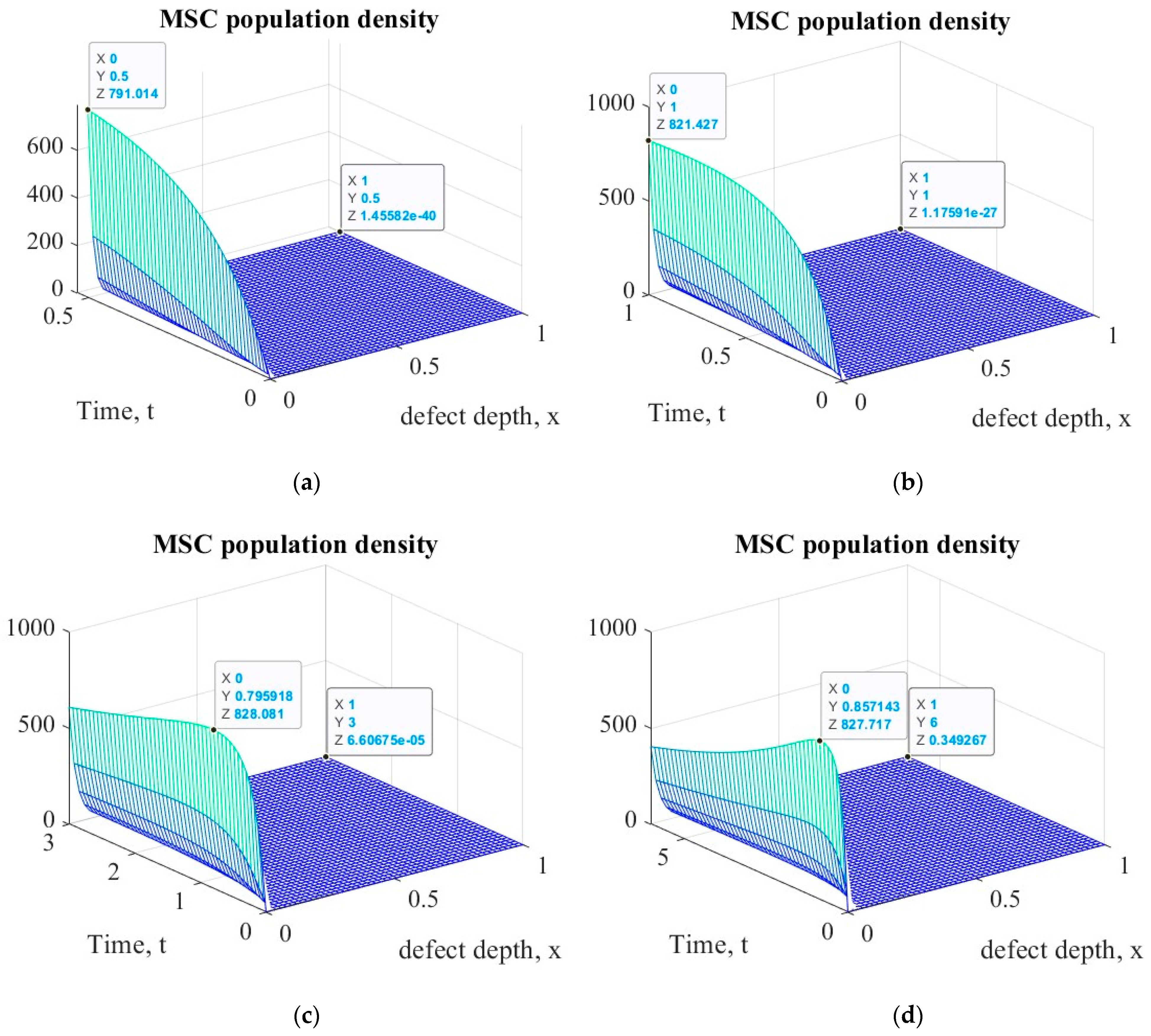
It is easy to see that ECM density () in the time interval increases nonlinearly over the entire defect depth . At the same time, and change nonlinearly both at point and at . Up to a certain point in time at point an increase in MSC population density ( occurs, after which it has a tendency to decrease. Chondrocyte population density ( changes similarly; however, its decrease at point begins to be observed a little later.
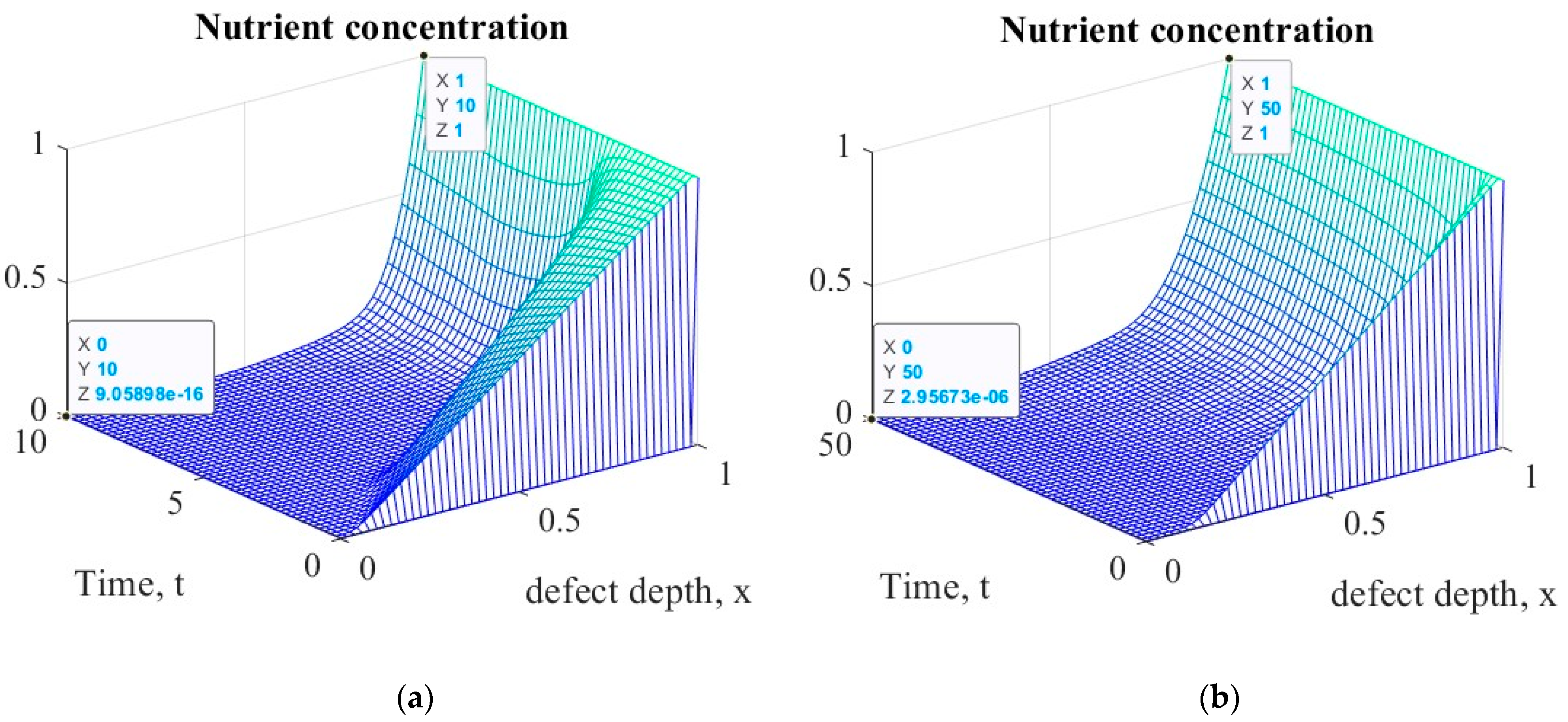
It is also necessary to note the implicit nonlinear nature of the change in the concentration of growth factors FGF-1 and BMP-2 in the considered period of time and a pronounced pattern of changes in the concentration of nutrients (
). The graphs of function
, presented in
Figure 4, indicate that, at the beginning of the regenerative rehabilitation process, nutrients are consumed in small quantities; however, from a certain point in time (in this case at
), their consumption becomes quite intense, starting from the defect surface, and they practically cease to reach the area close to the subchondral plate.
Analysis of the graphs presented in
Figure 7 and the data presented in
Table 2 allows us to note that, during a long period of AC regenerative rehabilitation, significant changes occur in the area of tissue being restored. The ECM formation occurs not only on the defect surface but also in the region of the subchondral bone. In this case, the ECM first begins to intensively form in the articular surface area, and later this process extends into the defect depth. At some point in time, the ECM density on the surface reaches a certain maximum value, after which it begins to decrease. At the same time, ECM density at the border with the subchondral plate increases constantly and, within the framework of the studied mathematical model, tends to equalize in depth over a long period of time. However, in reality, the AC density has a gradient structure similar in character to that shown in
Figure 7c,d.
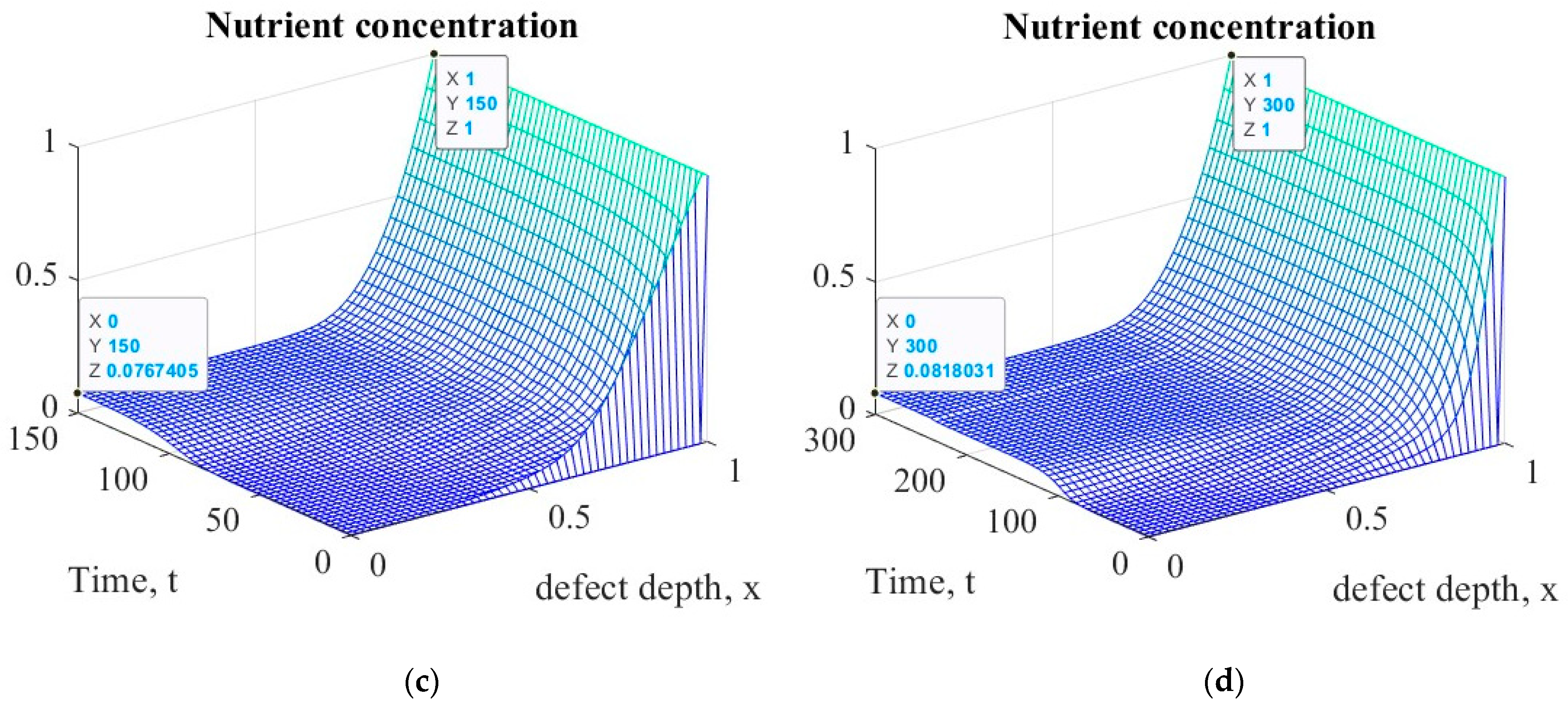
Analysis of the numerical experiment results to assess the long-term results of AC regenerative rehabilitation indicates that this process is supported by the supply of nutrients from the synovial fluid to the defect area. In this case, after the formation of ECM on the surface with a certain maximum density, its elements begin to diffuse into the depth of the defect along with the remaining nutrients. At some point in time, a sufficient amount of nutrients is concentrated in the subchondral plate area, which is necessary both for the formation of a new matrix and for supporting the viability of cells in the previously formed matrix. This is confirmed by the presence of a characteristic plateau in the graphs shown in
Figure 10c,d.
It should be noted that all the results in this series of numerical experiments were obtained taking into account the mechanical stimulation applied throughout the entire period of regenerative rehabilitation, applied at the initial stage to the explant, and subsequently to the tissue formed in the defect area. Since it is very difficult to imagine the constant use of rehabilitation procedures for a long period of time, it can be conditionally assumed that at the initial stage they are created artificially according to rehabilitation protocols and then applied in the process of the patient’s daily physical activity.
4. Conclusions
This study was carried out on the basis of a mathematical model for the AC regenerative regeneration, which is quite simple from the point of view of the structure but difficult for practical implementation even with the use of modern computer systems and software environments. The main problem to be solved was the presence in the nonlinear partial differential equations representing the model of Heaviside step functions, whose arguments, in turn, are functions of state variables. However, two series of solutions of such systems were obtained by the finite element method in the Matlab environment using the built-in m-function “pdepe” on a hybrid supercomputer cluster (x86/CUDA).
The mathematical model of the AC regenerative rehabilitation process provides for the possibility of implementing one of the technologies, i.e., ASIT, ACIT, or a combination of the two, as well as the possibility of using mechanical stimulation for the tissue being restored. In numerical experiments, all possible options were studied, and it was found that their nature is determined, first of all, by the model limitations and, therefore, practically does not depend on the type of technology being implemented. In this regard, this paper illustrates the results of a mathematical model study for only one option: ASIT under mechanical tissue stimulation. At the same time, it should be noted that each of these technologies allows for a different intensity of changes in the process state parameters, which can be evaluated in detail in future studies.
In this study, we focused mainly on short-term and long-term results of changes in ECM density in the regenerative rehabilitation process for a local AC defect. It was found that in the early stages of the process, the production of ECM is initiated in the subchondral plate region, due to the presence of a certain amount of chondrocytes in that region and the concentration of nutrients necessary for synthesis. Gradually, this process changes its direction, and the matrix begins to be produced more intensively near the defect surface. Nevertheless, the results of the experiments show that, at least for a month and a half, ECM is more actively produced in the depth of the defect. Then, within 1–2 months, the intensity of ECM formation in the depth and on the defect surface are approximately the same order with an increase trend in the surface zone, which can be explained by a limited amount of nutrients in the defect depth.
Furthermore, the process of ECM production depends on the diffusion of MSCs into the defect area, their proliferation, differentiation into chondrocytes, and death. Taking into account the fact that nutrients are constantly supplied to the defect area but in a limited amount, the intensity of ECM production in a certain area of space also turns out to be limited. In this regard, its density in different zones of the defect has different values. It is only after reaching the highest density value on the defect surface that the ECM formation front begins to shift into the depth of the defect, which is clearly seen in the graphs presented in
Figure 7. Finally, in the long term, the ECM density, according to the numerical experiments results, should acquire a steady-state gradient structure, the stability of which will be provided by the diffusion of nutrients from the subchondral bone of MSCs and from the synovial fluid.
In general, our results do not contradict those previously obtained by M. Lutianov et al. [
56], but, in our opinion, they are more informative. In addition, in this study, we modeled the effect of mechanical stimulation on the intensity of AC regeneration. As a result of numerical experiments, it was found that an increase in the proliferation rate of MSCs and chondrocytes, the rate of differentiation of MSCs into chondrocytes, and an increase in cell viability make it possible to intensify the regenerative process at early stages. The effects shown at the same time in the long term in this study could not be identified. However, presumably, these effects are objectively present and can be explained, at least, by an increase in the supply of nutrients to the AC during its periodic compression, both in clinical rehabilitation and in daily life. However, within the framework of the mathematical model used in this study, we were not able to reasonably explain the need to delay the start of mechanical stimulation, which is usually provided for in the protocols for performing the rehabilitation procedures.
The results of numerical experiments indicate that the regenerative rehabilitation of AC defects, even with the use of modern technologies, is a rather long process. So, for example, an elementary analysis of the graphs presented in
Figure 7d shows that, within the framework of the model we used, this process cannot be considered completed even after 9 years, since the optimal ECM gradient structure has not yet been fully formed during this time. That is, theoretically, this process can continue for some period of time. This shortcoming of the model, in principle, can be easily eliminated if certain temporal or quantitative restrictions are introduced on the parameters that determine the course of the process.
Thus, the results of the study presented in this paper allow us to draw the following generalized conclusions:
The mathematical model of regenerative rehabilitation studied in this work as a whole adequately reflects the course of AC regenerative processes in the implementation of cellular technologies with parallel physical stimulation of the formed tissue.
Estimates obtained using the study of such a model will allow more reasonable planning of the regenerative rehabilitation protocols, at least for experimental studies in vivo.
In order to increase the level of adequacy of the mathematical model, it is necessary, as a result of experimental studies in vitro and in vivo, to evaluate the rate of proliferation and differentiation of chondrogenic cells depending on the tissue microenvironment state, and on the type and intensity of stimulation.
In the refined mathematical model, it is necessary to provide for the possibility of fibrocartilage formation in the regenerative rehabilitation process, taking into consideration its possible hyalinization, as well as changes in ECM density, considering scaffold degradation.


