Abstract
Over half a century from the discovery of gamma-ray bursts (GRBs), the dominant radiation mechanism responsible for their bright and highly variable prompt emission remains poorly understood. Spectral information alone has proven insufficient for understanding the composition and main energy dissipation mechanism in GRB jets. High-sensitivity polarimetric observations from upcoming instruments in this decade may help answer such key questions in GRB physics. This article reviews the current status of prompt GRB polarization measurements and provides comprehensive predictions from theoretical models. A concise overview of the fundamental questions in prompt GRB physics is provided. Important developments in gamma-ray polarimetry including a critical overview of different past instruments are presented. Theoretical predictions for different radiation mechanisms and jet structures are confronted with time-integrated and time-resolved measurements. The current status and capabilities of upcoming instruments regarding the prompt emission are presented. The very complimentary information that can be obtained from polarimetry of X-ray flares as well as reverse-shock and early to late forward-shock (afterglow) emissions are highlighted. Finally, promising directions for overcoming the inherent difficulties in obtaining statistically significant prompt-GRB polarization measurements are discussed, along with prospects for improvements in the theoretical modeling, which may lead to significant advances in the field.
1. Introduction
Gamma-ray bursts (GRBs) are one of the most energetic, and electromagnetically the brightest, transient phenomena in the Universe. They are the ideal test beds for understanding nature at its extreme that involves an explosive release of energy over a short timescale, producing a burst of -rays with an isotropic-equivalent luminosity of . It is now well established that most GRBs are cosmological sources and that they are powered by ultrarelativistic (with bulk Lorentz factors ) bipolar beamed outflows driven by a central engine–a compact object. The identity of the central engine, which could be either a black hole (BH) or a millisecond magnetar, is not entirely clear as the highly variable emission is produced far away from it at a radial distance of cm. The most luminous phase of the burst, referred to as the “prompt” phase is short lived with a bimodal duration distribution, where the short GRBs have typical durations of s and the long GRBs typically last for s while the dividing line sits at s [1]. These two classes of GRBs are also distinct spectrally, with the short GRBs being spectrally harder as compared to the long GRBs that produce softer -rays. Other clues, e.g., the association of long-soft GRBs with star-forming regions [2] and type-Ib/c supernovae [3,4,5] and that of the short-hard GRBs with early type galaxies [6,7] lead to the identification of two distinct progenitors. The long-soft GRBs are associated with the core-collapse of massive () Wolf–Rayet stars [8], whereas the short-hard GRBs were theorized to originate in compact object mergers, namely, that of two neutron stars (NSs) or a NS-BH pair [9,10]. The unequivocal proof of the latter association had to wait until the gravitational wave (GW) detectors, LIGO and Virgo, became operational, which led to the coincident detection of GWs from the merger of two NSs and a short-hard GRB by Fermi-GBM and the INTEGRAL-ACS from GW 170817/GRB 170817A [11,12].
Although the global picture is fairly clear, the details of the energy dissipation process, the exact radiation mechanism, and the transfer of radiation in the highly dynamical flow remain poorly understood. All of these different processes combine to produce a non-thermal spectrum that is often well described by the Band function [13], an empirical fit to the spectrum featuring a smoothly broken power law. In space, which indicates the observed energy flux around the frequency with being the spectral flux density, this break manifests as a peak at the mean photon energy keV, which also represents the energy at which most of the energy of the burst is released, and the asymptotic power-law photon indices below and above the break energy have mean values of and , respectively [14,15]. After decades of spectral modeling of the prompt emission, the basic questions of GRB physics remain unanswered, and it is becoming challenging to advance our understanding with spectral modeling alone.
An exciting opportunity was presented by the claimed detection of high levels of linear polarization, with , in GRB 021206 [16]. Although this result had a detection significance of , further scrutiny by other works [17,18] cast irrevocable doubts and ultimately refuted the final result. Nevertheless, this one result initiated a vigorous theoretical effort to understand the polarization of prompt GRB emission with the expectation that highly sensitive measurements will be able to resolve many of the outstanding questions of GRB physics. Over the past several years, the number of prompt GRB polarization measurements (in some cases time-resolved) have grown; however, the main results remain inconclusive due to inherent difficulties in obtaining highly statistically significant measurements. Therefore, it is hoped that the next generation of -ray polarimeters that will be launched in this decade will provide further important clues.
The main objectives of this review were to provide a concise yet comprehensive overview of the current status of theoretical developments as well as observations in the field of prompt GRB polarization and also to highlight the need for developing more sensitive instruments and better analysis tools, which are hoped to yield statistically significant measurements in the coming decade. Many points presented here have also been covered in earlier reviews on the topic e.g., [19,20,21,22,23,24]. This review begins with a summary of the fundamental questions in GRB physics (Section 2) that can be addressed with measurements of linear polarization along with insights gained from prompt GRB spectral modeling. These include the outflow composition and dynamics (Section 2.1), energy dissipation mechanisms (Section 2.2), radiation mechanisms (Section 2.3), and the angular structure of the outflow (Section 2.4). An overview of -ray polarimetry is presented in Section 3, which includes the fundamental principles of -ray polarization measurement (Section 3.1) and a summary of the different detectors that have been used for GRB polarimetry (Section 3.3). The theory of GRB polarization is presented next in Section 4, which covers several topics, such as polarization from uniform (Section 4.1) and structured (Section 4.2) jets with different radiation mechanisms, temporal evolution of polarization (Section 4.3), polarization arising from multiple overlapping pulses (Section 4.4), the most likely polarization for a given radiation mechanism (Section 4.5), and the energy dependence of polarization (Section 4.6). The current status of prompt GRB polarization measurements is presented next, which includes time-integrated (Section 5.1), time-resolved (Section 5.2), and energy-resolved (Section 5.3) measurements. The importance of polarization measurements from the other phases of the burst, namely, X-ray flares, reverse-shock emission (optical flash and radio flare), and forward-shock emission, which also probe the properties of the GRB outflow, is emphasized in Section 6. Finally, Section 7 touches upon the outlook for this decade, which will see the launch of more sensitive instruments (Section 7.1). The predicted performance of some is compared in Section 7.2. This review concludes by offering some suggestions for improvements in the polarization data analysis (Section 7.3) and its theoretical modeling (Section 7.4).
2. Key Questions That Can Be Addressed with GRB Polarization
Measurements of the prompt GRB polarization may help shed light on many critical aspects of the relativistic outflow whose knowledge has evaded us so far. Below, we summarize key open questions in GRB physics, which can be probed with spectro-polarimetric observations. More detailed reviews and discussions of these topics can be found in other review articles (e.g., [25,26,27,28,29]). Theoretical modeling of prompt GRB polarization and comprehensive results are provided in Section 4.
2.1. What Are the Outflow Composition and Dynamics?
The main dissipation and radiation mechanisms that produce the GRB prompt emission are dictated by the composition of the outflow. The two most widely discussed scenarios invoke an outflow that is either kinetic-energy-dominated (KED) [30] or Poynting-flux-dominated (PFD) [31,32]. In the former, most of the energy is initially thermal (fireball) and is eventually transferred to the kinetic energy of the cold baryons, while in the latter the main energy reservoir is the (likely ordered) magnetic field that drives the expansion and acceleration of the flow. If the radiation mechanism is indeed synchrotron (see Section 2.3), then the level of polarization in both types of flows depends on the structure of the magnetic field that is either generated in situ, e.g., in internal shocks in a KED flow, or survives at large distances from the central engine, which could happen in both types of flows. Our theoretical understanding of the B-field structure in the emission region in a given type of flow is still limited and rather speculative. Any measurement of polarization will put strong constraints on the B-field structure. Therefore, in combination with polarization measurements, spectral and temporal (pulse profiles) modeling will allow us to constrain the composition.
The distinction between a KED and PFD flow can be conveniently parameterized using the magnetization parameter,
which is defined as the ratio of the comoving (all quantities measured in the comoving/fluid frame are primed) magnetic field enthalpy density, , to that of matter, or when it is cold (). Here is the magnetic field strength, and we assumed here for simplicity that the baryons dominate the total rest mass with density , where is the particle number density, is the proton mass, and c is the speed of light. The baryons were assumed to be cold with an adiabatic index ( for a relativistic fluid) and negligible pressure when compared with the particle inertia. A KED flow will have ; magnetic fields, if present, are weak and randomly oriented with short coherence length scales and are unimportant in governing the dynamics of the outflow. On the other hand, a PFD flow will have , and the magnetic field is much more ordered where it is responsible for accelerating the flow.
A prime example of a KED flow is the standard “fireball” scenario [33,34], in which total energy E is released close to the central engine, launching a radiation-dominated and optically thick outflow, with Thomson optical depth . The temperature at the base of the flow is typically MeV, which leads to copious production of -pairs via -annihilation that further enhances the optical depth. The enormous radiation pressure causes the flow to expand adiabatically, thereby converting the radiation field energy to the kinetic energy of baryons, which are inefficient radiators due to their large Thomson cross-sections. The bulk Lorentz factor (LF) of the fireball grows linearly with the radius, , where is the launching radius, while its comoving temperature declines as . The amount of baryon loading, i.e., the amount of baryons with total mass entrained in the flow of given energy E, determines the terminal LF, , which is attained at the saturation radius at which point the growth in the bulk saturates and the flow simply coasts at . The kinetic energy of the baryons is tapped at a large distance () from the central engine via internal shocks (see below).
In a PFD flow, large-scale magnetic fields propagate outwards from the central engine with an angular coherence scale , where represents the characteristic angular scale over which the flow is causally connected and, as discussed later, also the angular scale into which the emitted radiation is beamed towards the observer from a relativistic flow. While the fireball scenario is well agreed upon and has enjoyed many successes since it is fairly robust, no such standard model exists for a magnetized outflow to explain GRB properties. In several works (e.g., [35,36,37,38,39]), ideal-MHD models for a steady-state, axisymmetric, and non-dissipative outflow have been developed in which the flow expands adiabatically due to magnetic stresses. The flow is launched highly magnetized near the light cylinder radius, , with and bulk LF . As the flow expands, its magnetization declines with radius, and in the case of a radial wind (i.e., unconfined, with a negligible external pressure) the flow is limited to a terminal LF of where the corresponding magnetization of the flow is [40]. For weak external confinement (an external pressure profile with , where is the distance from the central source along the jet’s symmetry axis and is the cylindrical radius), the acceleration saturates at a terminal LF of and magnetization where is the jet’s asymptotic half-opening angle [41]. For strong external confinement ( with ), the jet maintains lateral causal contact and equilibrium, leading , which saturates at , , and . Since prompt GRB observations demand the dissipation region to be expanding ultrarelativistically with , to avoid the compactness problem [25,42], and afterglow observations suggest that typically , which implies in GRBs. This suggests that the weakly confined regime is most relevant for GRBs; however, it implies , which suppresses internal shocks. It has been pointed out [43,44] that the sharp drop in the surrounding (lateral) pressure as the jet exits the progenitor star in long GRBs can lead to along with a more modest asymptotic magnetization , but even then internal shocks remain inefficient.
When the steady-state assumption is relaxed, alternative models that consider an impulsive and highly variable flow yield a much larger terminal LF with and may achieve or even under certain conditions [45,46]. In this scenario, a thin shell of initial width is accelerated due to magnetic pressure gradients that causes its bulk LF to grow as , where , while its magnetization drops as . The bulk LF of the shell saturates at at which point its and . For , the magnetization continues to drop further as as the shell starts to spread radially. For a large number of shells initially separated by , the radial expansion is limited as neighboring shells collide and one expects an asymptotic mean magnetization of . This scenario offers the dual possibility of magnetic energy dissipation via MHD instabilities when at as well as kinetic energy dissipation via internal shocks when at .
Similar outflow dynamics were obtained in a popular model that makes the magnetohydrodynamic (MHD) approximation and features a striped-wind magnetic field structure [47,48,49,50,51], in which magnetic field lines reverse polarity over a characteristic length scale cm. Here, is the central engine’s angular frequency with P being its rotational period. Close to the central engine the flow may be accelerated by magneto-centrifugal, and to some extent, thermal acceleration. At distances larger than the Alfvén radius, where , these effects are negligible, and when collimation-induced acceleration is ineffective then the properties of the flow can be described using radial dynamics. If a reasonable fraction (the usual assumption is approximately half) of the dissipated energy in the flow goes towards its acceleration, conservation of the total specific energy, while ignoring any radiative losses, yields the relation for a cold flow, which simplifies to for . At the Alfvén radius, the four velocity of the flow is , which implies that and . The terminal LF is achieved at the saturation radius when , at which point . In this scenario, the saturation radius is given by cm, where is a measure of the reconnection rate where it quantifies the plasma inflow velocity into the reconnection layer in terms of the Alfvén speed. For magnetized flows, , which approaches the speed of light for . Beyond the Alfvén radius, the bulk LF grows as a power law in radius, with , while the magnetization declines as .
In the regime of high magnetization (), an alternative model that does not make the MHD approximation was considered by Lyutikov and Blandford [32] and Lyutikov [52].
2.2. How and Where Is the Energy Dissipated?
The composition of the outflow has a strong impact on the dominant energy dissipation channel. To produce the prompt GRB emission, the baryonic electrons as well as any -pairs, which are the primary radiators, cannot be cold, and they need to be accelerated or heated to raise their internal energy. The observed photon energy spectrum is not only shaped by the underlying radiation mechanism but also the radial location in the flow where energy is dissipated. If most of the energy is dissipated much below the photospheric radius, at , where the Thomson optical depth of the flow is and where the radiation field and particles are tightly coupled via Compton scattering (baryons are coupled with the leptons via Coulombic interactions) and assume a thermal distribution, the final outcome is a quasi-thermal spectrum [31,33,34]. The observed spectrum in this case is not a perfect blackbody, due to the observer seeing different parts of the jet with different Doppler boosts, but close to one with a low-energy (below the spectral peak energy) photon index , which is softer from expected for a Rayleigh–Jeans thermal spectrum [53,54]. If instead most of the energy is dissipated in the optically thin () parts of the flow, then a non-thermal spectrum emerges. When the flow is continuously heated across the photosphere, the final spectrum is a combination of two components: quasi-thermal and non-thermal.
If the flow is uniform (i.e., quasi-spherical with negligible angular dependence within angles of around the line of sight), then any thermal component will show negligible polarization as there is no preferred direction for the polarization vector to align with. Even if different parts of the flow may be significantly polarized at the photosphere [55], the net polarization averages out to zero after integrating over the GRB image on the sky. However, angular structure in the flow properties can lead to modest () polarization [24,56,57,58]. The polarization of the non-thermal spectral component ultimately depends on the radiation mechanism, discussed in Section 2.3.
In a KED flow, after an initial phase of rapid acceleration of the fireball when the bulk LF saturates, the particles are cold in the comoving frame with negligible pressure (). The energy of the flow is dominated by the kinetic energy of the baryons, which is very ordered. To produce any radiation, particle motion needs to be randomized. A simple and robust method to achieve that is via shocks. The canonical model of internal shocks [30,59,60,61] posits that the central engine accretes intermittently and ejects shells of matter that are initially separated by a typical length scale and have fluctuations in their bulk LFs of order , with being the mean bulk LF. Here, is the observed variability of the prompt emission lightcurve, and z is the redshift of the source. Typically, cm and so that the acceleration saturates at cm. For , faster-moving shells catch up from behind with slower ones and collide to dissipate their kinetic energy at internal shocks occurring at the dissipation radius of cm.
When the shells collide, a double-shock structure forms with a forward shock going into the slower shell and accelerating it while a reverse shock goes into the faster shell and decelerates it. These shocks heat a fraction of the electrons into a power-law energy distribution, with for , where these electrons hold a fraction of the total internal energy density behind the shock. The LF of the minimal energy electrons, (for ), depends on the relative bulk LF, , of the upstream to downstream matter across the relevant shock. A fraction of the internal energy density behind the shock is held by the shock-generated magnetic field of strength G. More generally, one can express the comoving magnetic field in terms of the radius and outflow Lorentz factor and magnetization at that radius, as well as the observed isotropic equivalent -ray luminosity, , and the -ray emission efficiency, (i.e., fraction of the total outflow energy channeled into gamma-rays), G. The exact structure of the magnetic field is still an open question, but it has been argued that streaming instabilities [62,63,64,65,66], e.g., the relativistic two-stream and/or Weibel (filamentation) instability, are responsible for generating a small-scale field with coherence scale on the order of the electron and/or proton skin depth, where is the plasma frequency, which depends on the particle number density ; mass m is the particle mass; and e is the elementary charge. Since the coherence length of the shock-generated field is much smaller than the angular size of the beaming cone (), the net polarization is limited to .
Alternatively, interactions of the shock with density inhomogeneities in the upstream can cause macroscopic turbulence in the downstream (e.g., excited by the Richtmyer–Meshkov instability), which can in turn amplify a shock-compressed large-scale upstream magnetic field to near-equipartition with the downstream turbulent motions [67,68,69,70,71,72]. The dynamo-amplified magnetic field is expected to form multiple mutually incoherent patches (with angular sizes up to a fraction of the visible region) in which the field is largely ordered. The expected polarization, after averaging over such patches in the observed region, is typically expected to be small, with [69].
As mentioned earlier, in a PFD flow, the main dissipation channel is magnetic reconnection and /or MHD instabilities. Both of these are non-ideal effects that cannot be treated in an ideal MHD formalism. Magnetic field energy is dissipated when opposite polarity field lines reconnect, which leads to acceleration of electrons that then cool by either emitting synchrotron radiation outside of the reconnection sites or inverse-Compton scattering of either synchrotron photons or a pre-existing radiation field advected with the flow. Exactly where dissipation commences depends on the initial magnetic field geometry in the flow as the field lines expand outward from the central engine to larger distances [73]. If the flow is axisymmetric and is not permeated by polarity-switching field lines, magnetic energy can still be dissipated due to current-driven instabilities, e.g., the kink instability [74,75,76,77]. Such an instability may also occur at the interface between the jet and the confining medium, e.g., the stellar interior of a Wolf–Rayet star in long-soft GRBs [78] and the dynamically ejected wind during a binary neutron star merger in short-hard GRBs. Magnetic field lines that reverse polarity on some characteristic length scale can be embedded into the outflow in a variety of ways [79]. These can indeed be injected at the base of the flow where field polarity reversals are obtained in the accretion disk due to the magnetorotational instability, as demonstrated in several shearing-box numerical MHD simulations [80] as well as in global simulations of black hole accretion [81]. Depending on how particles are heated/accelerated when magnetic energy is dissipated, as the flow becomes optically-thin, as discussed in the next section, the polarization will be energy dependent and can be if synchrotron emission dominates and the B-field angular coherence length near the line of sight is .
In the striped-wind model [49,50,82], magnetic dissipation commences beyond the Alfvén radius and becomes the dominant contributor towards flow acceleration. Below the Alfvén radius the flow is accelerated due to magneto-centrifugual effects as well as collimation provided by the confining medium [39,83]. If the confining medium has a sharp outer boundary (e.g., the edge of the massive star progenitor for a long GRB), then as the jet breaks out of the confining medium, the flow becomes conical and expands ballistically. The sudden loss of pressure also leads to some further acceleration via the mechanism of rarefaction acceleration [44] that operates in PFD relativistic jets. While these ideal MHD processes may continue to operate at length scales relevant for prompt GRB emission, magnetic reconnection in a striped wind provides a source for gradual acceleration out to the saturation radius . Beyond this radius magnetic reconnection subsides, and therefore acceleration ceases and the flow starts to coast. When the prompt emission is produced in an accelerating flow, the degree of polarization is not affected. Instead, the duration of the pulses becomes shorter in comparison to that obtained in a coasting flow—see, e.g., [84].
Other variants of the PFD model, as presented above, include the internal-collision-induced magnetic reconnection and turbulent (ICMART) model [85], in which high- shells are intermittently ejected by the central engine that dissipate their energy at cm, where collision-induced magnetic reconnection and turbulence radiates away the magnetic energy and reduces the initially high magnetization of the ejecta to order unity. The expected polarization from an ICMART event has been presented in Deng et al. [86] using 3D numerical MHD simulations where they also find a change in polarization angle.
2.3. What Radiation Mechanism Produces the Band-like GRB Spectrum?
Few radiation mechanisms have been proposed to explain the Band-like spectrum of prompt emission, the most popular being synchrotron and inverse-Compton. Below, we present a concise summary of the different proposed mechanisms and show the expected polarization in Figure 1.
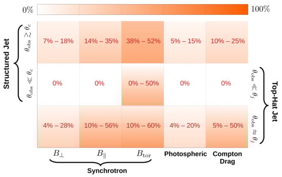
Figure 1.
Approximate degree of polarization for different radiation mechanisms and jet structures [24]. If the emission is synchrotron then polarization for different B-field configurations is given (assuming ). For each jet structure, a distinction is made between two cases: (i) when the observer’s viewing angle () is much smaller than the half-opening angle () of a top-hat jet or, in the case of a structured jet, if it is much smaller than the core angle () and (ii) when is close to , i.e., the edge of the jet. For a structured jet, can exceed by an order unity factor before the fluence starts to drop significantly. When , the minimum value of polarization can be zero in all cases, except for , for a pulse with a given , where is the ratio of the angular sizes of the jet and of the beaming cone. Different pulses may have slightly different (typically with a similar but different ), which on average would yield a finite polarization. The quoted lower range reflects this mean value (see [24] for more details). For the case, when due to symmetry and otherwise, while at .
2.3.1. Optically-Thin Synchrotron Emission
Relativistic electrons gyrating around magnetic field lines cool by emitting synchrotron photons. When the energy distribution of these electrons is described by a power law, e.g., that obtained at collisionless internal shocks due to Fermi acceleration, the emerging synchrotron spectrum is described by multiple power-law segments that join at characteristic break energies [87,88]. These correspond to the synchrotron frequency, , of minimal-energy electrons with LF and the cooling frequency, , of electrons that are cooling at the dynamical time, . Here, is the comoving magnetic field, and is the Thomson cross-section. The high radiative efficiency of prompt emission demands that the electrons be in the fast-cooling regime for which and the spectrum peaks at . In this case, the spectrum below the peak energy has a photon index for and for . Above the peak energy, the photon index is where p is the power-law index of the electron distribution.
While synchrotron emission is still regarded as the default emission mechanism, the basic “vanilla” model has been argued to be not as robust as previously thought. First, its predictions have been challenged by a small fraction of GRBs that showed harder low-energy () spectral slopes with [89,90,91,92], often identified as the synchrotron line of death. Some possible alternatives that have been suggested to resolve this discrepancy include anisotropic electron pitch angle distribution and synchrotron self-absorption [93], jitter radiation [94], and photospheric emission [95]. The line-of-death violation is generally derived by fitting the empirical Band-function to the observed spectrum. When synthetic synchrotron spectra (after having convolved with the energy response of a detector) are fit with the Band-function, an even softer is found due to the detector’s limited energy range (e.g., Fermi/GBM [96]), which does not quite probe the asymptotic value of . Since a significant fraction of GRBs show low-energy spectral indices that are harder than this value, it might indicate that another spectral component is possibly contributing at low energies and offsetting the spectral slope. Second, the spectral peak energy in the cosmological rest-frame of the source is given by , which depends on a combination of , , and to yield the measured peak energy in the range MeV [97] with a possible peak around [98]. Given that all of these quantities can vary substantially between different bursts, the synchrotron model does not offer any characteristic energy scale at which most of the energy is radiated in the event that the distribution indeed narrowly peaks around [99]. Third, the synchrotron model predicts wider spectral peaks than that obtained by fitting the Band-function to observations [100]. This issue has now been demonstrated for a large sample of GRBs where the spectral widths obtained with the simplest synchrotron model yielding the narrowest spectral peak, e.g., a slow-cooling Maxwellian distribution of electrons, is inconsistent with most of the GRBs [101,102]. Moreover, it is rather easy to get a wider spectral peak by having, e.g., fast-cooling particles, variable magnetic fields, etc., but it is much harder to obtain narrower peaks.
Several works that find the synchrotron model to be inconsistent with observations invariably use empirical models, e.g., the Band-function, a smoothly-broken power law, to determine low-energy spectral slopes and peak widths. This may become a problem in instances where such models are unable to capture the intrinsic complexity of the underlying data. Therefore, an arguably better approach is to directly fit physical models to the raw data to derive spectral parameters and remove any bias [103,104,105,106]. Such an approach has led to alleviating some of the issues encountered by the optically thin synchrotron model, where it was shown that direct spectral fits (in count space rather than energy space) with synchrotron emission from cooling power-law electrons can explain the low-energy spectral slopes as well as the spectral width of the peak [107].
Magnetic Field Structure
If the coherence length of the magnetic field is larger than the gyroradius of particles, the structure of the magnetic field in the dissipation region does not affect the spectrum or the pulse profile. However, it significantly affects the level of polarization. Therefore, spectro-polarimetric observations that strongly indicate synchrotron emission as the underlying radiation mechanism can be used to also determine the magnetic field structure. At least four physically motivated axisymmetric magnetic field structures, and the emergent synchrotron polarization, have been discussed in the literature [108,109,110,111]:
- : An ordered magnetic field with angular coherence length , where is the angular size of the beaming cone. It is envisioned that the jet surface is filled with several small radiating patches of angular size much smaller than the jet aperture and that these are pervaded by mutually incoherent ordered magnetic fields. In this way, such a field configuration as a whole remains axisymmetric in a statistical sense (despite having a local preferred direction for a given line of sight, namely, the ordered field direction at that line of sight) and also different from a globally ordered B-field. This type of field structure was motivated by the high-polarization claim of [16] in GRB 021206 and by the notion that the local synchrotron polarization can be very high with . Magnetic fields with sufficiently large coherence lengths that are not globally ordered can be advected with the flow from the central engine where their length scale is altered en route to the emission site due to hydromagnetic effects.
- : A random magnetic field (i.e., with ) confined to the plane transverse to the local velocity vector of the fluid element in the flow. In many cases, the flow is assumed to be expanding radially, which is a good approximation when the prompt emission is generated since no significant lateral motion is expected at that time. This field structure is motivated by the theoretical predictions of small-scale magnetic fields generated by streaming instabilities at collisionless shocks [62,63,64,65,66].
- : An ordered field aligned along the local velocity vector of the outflow. This field structure presents the opposite extreme of , and in reality the shock-generated field may likely be (at least its emissivity-weighted mean value over the emitting region downstream of the shock) more isotropic than anisotropic whereby it would be a distribution in the parameter space (see, e.g., [109,112] in the context of afterglow collisionless shocks).
- : A globally ordered toroidal field symmetric around the jet symmetry axis. Such a field configuration naturally arises in a high magnetization flow in which the dynamically dominant field is anchored either to the rotating central engine or in the accretion disk. The azimuthal motion of the magnetic footpoints tightly winds up the field around the axis of rotation, which is also the direction along which the relativistic jet is launched. Due to magnetic flux conservation, the poloidal component declines () more rapidly as compared to the toroidal component () as the flow expands. Therefore, at large distances from the central engine the toroidal field component dominates.
2.3.2. Inverse-Compton Emission
If the energy density of the (isotropic) radiation field (, where is the isotropic-equivalent luminosity) advected with the flow is much larger than that of the magnetic field (), relativistic particles with LF cool predominantly by inverse-Compton upscattering softer seed photons, with energy , to higher energies with a mean value (for an isotropic seed photon field in the comoving frame), . When the Thomson optical depth of the flow is , these seed photons undergo multiple Compton scatterings, where the process is usually referred to as Comptonization, until they are able to stream freely when . Comptonization has been argued as a promising alternative to optically thin synchrotron emission where it is able to explain a broader range of low-energy spectral slopes, provide a characteristic energy scale for the peak of the emission, and yield narrower spectral peaks [99,113] It is the main radiation mechanism in a general class of models known as photospheric emission models in which the outflow is heated across the photosphere due to some internal dissipation.
At the base of the flow, where , the radiation field is thermalized and assumes a Planck spectrum. If the outflow remains non-dissipative the Planck spectrum is simply advected with the flow, cooled due to adiabatic expansion, and then released at the photosphere [33,34]. However, only a few GRBs show a clearly thermally dominated narrow spectral peak [114], whereas most have a broadened non-thermal spectrum with a low-energy photon index () softer than that obtained for the Planck spectrum (). In many cases, a sub-dominant thermal component in addition to the usual Band function has been identified [115,116]. These observations imply that photospheric emission plays an important role [117], but the pure thermal spectrum must be modified by dissipation across the photosphere [54,95,118,119,120]. Several theoretical works tried to understand the thermalization efficiency of different radiative process, e.g., Bremmstrahlung, cyclo-synchrotron, and double Compton, below the photosphere to explain the location of the spectral peak and the origin of the low-energy spectral slope e.g., [121,122,123].
While sub-photospheric dissipation and Comptonization is able to yield the typical low-energy slope, further dissipation near and above the photosphere is needed to generate the high-energy spectrum above the thermal spectral peak. This can be achieved by inverse-Compton scattering of the thermal peak photons by mildly relativistic electrons [24,100,124,125,126,127]. If the flow is uniform, the net polarization of the Comptonized spectrum is negligible due to random orientations of the polarization vector at each point of the flow, which, upon averaging over the visible part, adds up to zero polarization. Alternatively, if the flow has an angular structure, particularly in the bulk- profile, then net polarization as large as can be obtained [24,57].
2.3.3. Dissipative Jet: Hybrid Spectrum
If the jet is dissipative across the photosphere, a hybrid spectrum can emerge where the spectral peak is dominated by a quasi-thermal component but- the low and high-energy wings are dominated by non-thermal emission either from synchrotron or Comptonization. The final outcome depends on the nature of the dissipation and how that leads to particle acceleration/heating. Gill et al. [128], who carried out numerical simulations, and Beniamini and Giannios [129], who performed semi-analytic calculations, considered a steady PFD striped wind outflow, which is heated due to magnetic dissipation commencing at radii when the flow is optically thick to Thomson scattering with initial . At higher , and equivalently lower radii, the flow maintains thermal equilibrium while it is being accelerated due to gradual magnetic dissipation. Localized reconnecting layers accelerate the baryonic electrons, as well as any produced -pairs, into a relativistic power-law distribution. In this instance, since the flow is strongly magnetized with , the relativistic particles are predominantly cooled by synchrotron emission. The development of the spectrum as the flow expands is shown in the left panel of Figure 2 as a function of the total . The final observed spectrum is indeed Band-like, but it is different from the optically thin synchrotron spectrum even though by the end of the radially extended dissipation the total spectrum (energetically) is synchrotron dominated.
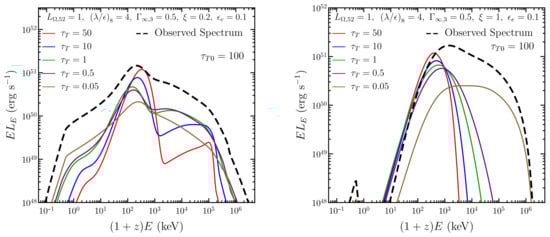
Figure 2.
Spectral evolution in a dissipative steady PFD striped wind flow, shown as a function of the Thomson optical depth as the jet is heated accross the photosphere. The spectra are shown for two different particle heating scenarios: (Left)—relativistic power-law particles produced by magnetic reconnection, and (Right)—mildly relativistic particles forming an almost mono-energetic distribution due to distributed heating and Compton cooling. The flow was evolved from initial until the total optical depth of baryonic electrons plus produced -pairs was much less than unity. The observed spectrum is effectively a sum over the optically thin spectra. See [128] for more details.
Alternatively, particle heating can occur in a distributed manner [31,124,126,130,131] throughout the whole causal region due to MHD instabilities. In this case, particles remain only mildly relativistic. Their mean energy is governed by a balance between (gradual and continuous) heating and Compton cooling, which leads to a mono-energetic distribution. The spectral evolution as the flow expands is shown in the right panel of Figure 2. In this case the high-energy spectrum is again Band-like, but unlike the previous case it is completely formed through Comptonization [124,126,131]. The mildly relativistic particles do produce some synchrotron emission but only at energies keV.
Both particle energization mechanims can give rise to a Band-like spectra; however, they can produce completely different energy-dependent polarization. In both, if the jet is uniform and can be approximated as part of a spherical flow (i.e., away from the jet edge in a top-hat jet), then no polarization is expected near the spectral peak, as it is dominated by the quasi-thermal component. In such a scenario, away from the peak, where the spectrum is dominated by non-thermal emission, it is possible to measure high polarization () if the emission is synchrotron and the flow has a large scale ordered magnetic field, e.g., a field. Other field configurations, namely, and , will yield vanishingly small net polarization. Alternatively, if the non-thermal component is produced by Comptonization, then the expected polarization is again almost zero. On the other hand, if the LOS passes near the sharp edge of a top-hat jet or the edge of the almost uniform core in a structured jet, then the entire spectrum with non-thermal emission from Comptonization can produce . Similarly, the non-thermal wings coming from synchrotron emission can now yield significant polarization with for and for , while again yields higher levels with .
2.3.4. Other Proposed Mechanisms
- (a)
- Compton Drag
This model envisions the propagation of the relativistic outflow in a dense bath of seed photons with energy that provide the drag for the expanding outflow whereby cold electrons in the outflow Compton upscatter soft photons [132,133]. The seed photons can be provided either by radiation from the associated supernova remnant that exploded a time few hours before the outflow is launched, or if is negligibly small then by the walls of the funnel that has been cleared in the massive star progenitor’s envelope by the jet-driven bow shock post core-collapse. These requirements limit the applicability of this model to only long-soft GRBs and do not explain how such an emission would arise in short-hard GRBs. This scenario presents an entirely non-dissipative flow, which is insensitive to the magnetization but yields a high () radiative efficiency. To produce the variability, the flow is required to be unsteady. The required in this model may make it difficult to produce prompt high-energy emission due to opacity to pair production.
When the prompt GRB emission originates inside the funnel, it is assumed that the funnel is pervaded by a blackbody radiation field emitted by the funnel walls. The spectral peak of the observed prompt emission is then simply the inverse-Compton scattered peak at energy , where is the bulk LF of the outflow. Inhomogeneity in the funnel temperature and bulk- of subsequent shells, which could also collide to produce internal shocks, gives rise to a Band-like broadened spectrum. The local polarization, i.e., from a given point on the outflow surface, can be as high as ; however, the net observable polarization, e.g., in a top-hat jet, is reduced to for a jet with [24]. If the jet is narrower than this with , then the net polarization can be much higher with [134]. However, such high polarization requires highly idealized assumptions that are hard to meet in reality.
- (b)
- Jitter Radiation
If the magnetic field coherence length is much smaller than the gyroradius of particles, then synchrotron radiation is not the correct description of the radiative mechanism by which relativistic electrons cool, as it assumes homogeneous fields. In this case, the particles experience small pitch-angle scattering where their motion is deflected by magnetic field inhomogeneities by angles that are smaller than the beaming cone of the emitted radiation (). This scenario has been proposed as a viable alternative to synchrotron radiation [94], where it has been shown to yield harder spectral slopes that cannot be obtained in optically-thin synchrotron emission. In addition, it can produce sharper spectral peaks as compared to synchrotron radiation, which agrees better with observations. The small-scale magnetic fields needed in this scenario may potentially be produced in relativistic collisionless shocks via the Weibel instability (although this may not be easy to achieve in practice; see e.g., [135]). The polarization when this small-scale field is confined to a slab normal to the local fluid velocity is calculated in [136,137], where it is shown that the maximum degree of polarization is obtained only at large viewing angles when the slab is viewed almost edge-on. For small viewing angles that apply to distant GRBs, the polarization is indeed very weak.
- (c)
- Synchrotron Self-Compton
Synchrotron self-Compton (SSC) emission has been considered in some works as a mechanism that could yield low-energy spectral slopes with photon indices as hard as , a change of over the synchrotron line of death [138]. This is facilitated by the fact that for typical values of the model parameters in the internal shock scenario, optically thin synchrotron emission peaks at much lower energies (at a few eV when the SSC peak is at ∼100 keV) and is mostly self-absorbed. One of the major drawbacks of this radiation mechanism is that it requires the synchrotron emission in the optical, which is the seed for the harder inverse-Compton emission, to be much (by a factor of ≳10) brighter than observed (or upper limits [139]). Otherwise, it requires the Compton-y parameter to exceed unity by the same factor, which is hard to accommodate while not strongly violating the total energy budget of the burst [140,141]. The energy-dependent local polarization for SSC in an ultrarelativistic spherical flow for two different ordered B-field configurations, one parallel and the other transverse to the local velocity vector, is calculated in [142], where they found that the local polarization can be as high as under simplifying assumptions.
2.4. What’s the Angular Structure of the Outflow?
The angular structure of the relativistic outflow in GRBs affects a number of important observables, such as prompt GRB pulse structure [84], polarization [24], afterglow lightcurve [143], and the detectability of distant GRBs [144,145]. Outflows in GRBs are collimated into narrowly beamed bipolar jets that have an angular scale , where in the simplest model of a uniform conical jet, also referred to as a top-hat Jet, represents a sharp edge. The notion of narrowly collimated jets in GRBs was first proposed by Rhoads [146], and it was later verified by observations of achromatic jet-breaks in the afterglow lightcurve that yielded (e.g., [147,148,149,150]). Since during the prompt emission phase and assuming that remains approximately the same, this yields . This geometric beaming futher implies that the true radiated energy of these bursts is much smaller [149] with erg, where is the geometric beaming fraction with the last equality valid for , erg is the isotropic-equivalent radiated energy, [] is the burst fluence, and is the luminosity distance. Since is much smaller than , the solid angle into which radiation from a spherical source is emitted, only observers whose line-of-sight (LOS) intersects the surface of the jet or passes very close to the jet edge can detect the GRB, which implies that the true rate of GRBs is enhanced by [149] over the observed rate.
A top-hat jet is clearly an idealization even though it is able to explain several features of the afterglow lightcurve. Numerical simulations of jets breaking out of the progenitor star for the long-soft GRBs [151,152,153,154,155] and that from the dynamical ejecta for the short-hard GRBs [155,156,157,158,159,160] find that these jets naturally develop angular structures by virtue of their interaction with the confining medium. If the true energy reservoir lies in a narrow range and the scatter in is instead caused by different viewing angles, then either the jet half-opening angle of a top-hat jet must be different in different GRBs or the jets are not uniform and must have an underlying angular profile for both the energy per unit solid angle, , and the (initial) bulk LF, . Such jets are commonly referred to as structured jets [161,162,163,164] and can be parameterized quite generally as a power law with and where with being the core angle. A constant true jet energy among a sample of GRBs implies that , a model referred to as a universal structured jet (USJ) [161,165,166,167], where it corresponds to equal energy per decade in and therefore reproduces jet breaks similar to those for a top-hat jet with (top-hat). This angular profile was used as an alternative model to the top-hat jet to explain the correlation [149] for the afterglow emission where is the jet-break time [161,167]. Other useful parameterizations of a structured jet include a Gaussian jet with , which is a slightly smoother (around the edges) and more realistic version of the top-hat jet.
The large distances of GRBs have precluded direct confirmation and constraints of the outflow’s angular structure. The main difficulty being the rather severe drop in fluence when they are observed outside of the almost uniform core. This changed recently with the afterglow observations of GRB170817A [12], the first-ever short-hard GRB detected coincidentally with GWs (GW 170817; [11]) from the merger of two neutron stars. Helped by its nearby distance of Mpc and an impressive broadband (from radio to X-rays) observational campaign (e.g., [168,169,170]), the afterglow observations led to the first direct and significant constraint on the angular structure of the relativistic jet (e.g., [170,171,172,173,174,175,176,177]). The afterglow from this source showed a peculiar shallow rise () to the lightcurve peak at days, after which point it declined steeply (). Several useful lessons were learned. First, it was shown that a top-hat jet can only explain the afterglow lightcurve near and after the lightcurve peak [177] and not the shallow rise for which a structured jet is needed. Second, both power-law- and Gaussian-structured jets can explain the afterglow of GW 170817, where for a power-law jet the angular structure profile requires and to explain all the observations [178].
While power-law- and Gaussian-structured jets remain most popular, a few other angular profiles have received some attention. Among them is the two-component jet model [150,179,180,181,182,183] that features a narrow uniform core with initial bulk LF surrounded by a wider uniform jet with . Nothing really guarantees or demands the outflow to be axisymmetric and uniform, in which case an outflow with small variations on small (≪1/) angular scales can be envisioned in the form of a “patchy shell” [184] or an outflow consisting for “mini-jets” [185], with the caveat that significant variations on such causally connected angular scales are rather easily washed out and hard to maintain. In case such variations do indeed persist, it could have important consequences for the time-resolved polarization and PA. For example, patches or mini-jets can have different polarization and/or PA due to mutually incoherent B-field configurations, which can lead to smaller net polarization and PA evolution.
3. Gamma-Ray Polarimetry
Despite the wealth of information that can be obtained from prompt GRB polarization, only a few measurements with modest statistical significance exist. Moreover, many of the results presented in the past were refuted by follow-up studies. A detailed overview of many of these measurements and their respective issues is provided in [186]. The two most recent measurements, by POLAR [187] and Astrosat CZT [188], furthermore appear to be incompatible with one another, indicating probable issues in at least one of these results as well. The lack of detailed measurements, and the many issues with them, result from both the difficulty in measuring -ray polarization as well as challenging data analysis at these energies. Below, we discus first the measurement principle, which causes many of the encountered issues. This is followed by a description of the different instruments that have been able to perform measurements to date.
3.1. Measurement Principles
The polarization of X-ray or -ray photons can be measured by studying the properties of the particles created during their interaction within the detector. For all the three possible interaction mechanisms, namely, the photo-electric effect, Compton scattering, and pair production, a dependency exists of the orientation of the outgoing products on the polarization vector of the incoming photon. This is illustrated in Figure 3 for the three processes. For the photo-electric effect, it is the azimuthal direction of the outgoing electron that shows a dependency on the polarization vector of the incoming photon; for Compton scattering, it is the azimuthal scattering angle of the photon; and for pair-production, it is the plane defined by the electron-positron pair.
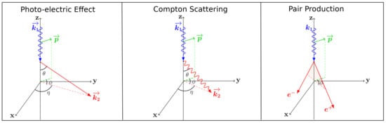
Figure 3.
Illustration of the angular dependency of the interaction product on the polarization vector of the incoming photon for the three interaction mechanisms: photo-electric effect (left), Compton scattering (middle), and pair production (right). The incoming photon is shown in blue, its polarization vector in green, and the secondary product(s) in red. The angle (as used in Equations (2) and (3)) is defined as the angle between the incoming photon direction and its secondary product. The angle (again as used in Equations (2) and (3)) is defined as the angle between the projections of the polarization vector and the momentum vector of the secondary product(s) onto the x-y plane. The angle is the azimuthal angle between the x-axis and the projection of the momentum vector of the secondary particle onto the x–y plane. The and angles can be directly measured in a detector, while is measured indirectly.
The differential cross section for photo-absorption (via the photo-electric effect) has a dependency on , which is defined as the azimuthal angle between the polarization vector of the incoming photon , as shown in Figure 3, and the projection of the velocity vector of the final state electron (where ) on to the plane normal to the momentum vector of the photon,
where is the unit solid angle, and the polar angle is given by . Similarly, for the differential cross section of Compton scattering the dependence on , here the angle between the polarization vector of the incoming photon and the projection of the momentum vector of the outgoing photon on to the plane normal to the momentum vector of the incoming photon, where as in Equation (2), is
Here, is the classical electron radius with e being the elementary charge, E is the initial photon energy, the final photon energy, and is the polar scattering angle.
Finally, for pair production the differential cross section is , where A is the polarization asymmetry of the conversion process (which has dependencies on the photon energy and properties of the target), and is the angle between the polarization vector of the incoming photon and the plane defined by the momentum vectors of the electron–positron pair, .
The general concept for polarimetry in the three energy regimes where these cross sections dominate is therefore similar: one needs to detect the interaction itself and subsequently track the secondary particle, be it an electron, photon, or electron–positron pair. This requirement indicates the first difficulty in polarimetry: simply absorbing the incoming photon flux, as is the case in, for example, standard spectrometry, is not sufficient. The requirement to track the secondary product significantly reduces the efficiency of the detector.
After measuring the properties of the secondary particles, a histogram of can be made, which shows a sinusoidal variation with a period of referred to as a modulation curve. The amplitude of this is proportional to the polarization degree (PD) and the phase related to the polarization angle (PA). As can be derived from, for example, the Compton scattering cross section, the amplitude for a polarized beam will depend on the energy of the incoming photons as well as on the polar scattering angle. Whereas the energy depends on the source, the polar scattering angle is indirectly influenced by the instrument design. For example, using a detector with a thin large surface perpendicular to the incoming flux, it is more likely to detect photons scattering with a polar angle of , which have a larger sensitivity to polarization than those scattering forward or backward. The relative amplitude, meaning the ratio of the amplitude of the sinusoidal over its mean, is directly proportional to the PD. The relative amplitude one detects for a polarized beam is known as the , and it depends on the source spectrum, source location in the sky, the instrument design, and the analysis. Although for specific circumstances the can be measured on the ground using, for example, mono-energetic beams with a specific incoming angle w.r.t the detector, its dependency on the energy, incoming angle, and instrument conditions, such as its temperature, implies that the required in the analysis of real sources can only be achieved using simulations. The large dependency on simulations provides a source for potential systematic errors in the analysis, which can easily dominate the statistical error in the measurements.
Additionally, it should be noted that in practice retrieving the polarization is significantly more complicated as both instrumental and geometrical effects (such as the incoming angle of the photons w.r.t. the detector and the presence and orientation of materials around the detector) are added to the polarization-induced signal in the modulation curve. In order to retrieve the polarization signal one can, for example, divide it by a simulated modulation curve for an unpolarized signal as illustrated in the first column of Figure 4. This method is often used, for example in [188]. A second option is to model these effects together with the signal and fit the uncorrected curve with this simulated response, as was for example done in [189]. In either case, it requires a highly detailed understanding of the instrument.
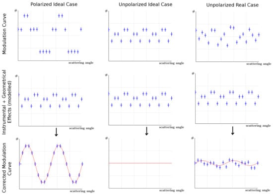
Figure 4.
Illustration of recovering the polarization signal from a raw modulation curve. The left column illustrates the ideal case with a high PD value, with a raw measured modulation curve (top), abd the perfectly simulated instrumental and geometrical effects (middle), which pollute the raw modulation curve. The (bottom) panel shows the modulation curve after correction from the instrumental and geometrical effects, which results in a perfect harmonic function. The middle column illustrates the same but for an unpolarized signal resulting in a flat distribution. The right column shows the same for an unpolarized signal; however, random small errors were added to the instrumental and geometrical effects, thereby simulating a non-perfect understanding of the instrument. The result is a non-flat distribution, which, when fitted, shows a low level of polarization.
In polarization analysis, any imperfections in modelling the instrument will likely result in an overestimation of the polarization. As illustrated in Figure 4, for a modulation curve resulting from an unpolarized flux, removing any instrumental effects from the modulation curve should result in a perfectly flat distribution. This is illustrated in the middle column of this figure. Any error in the model of the instrumental or geometrical effects will, however, result in a non-flat distribution, which, when fitted with a harmonic function, will result in some level of polarization to be detected. It is therefore in practice impossible to measure a PD of as it would require both an infinite amount of statistics, and more importantly, a perfect modelling of all the instrumental effects. On the other extreme, for a PD of , imperfections in the modelling can result in a lower amplitude, but can still also increase it further resulting in measuring a nonphysical PD. Overall, due to the nature of the measurement, both statistical and systematic errors tend to inflate the PD rather than decrease it. Since it is not possible to test the modelling of the instruments when in orbit, as there are no polarization calibration sources, this issue exists for all measurements and can only be minimized by extensive testing of the instrument both on the ground and in-orbit.
A final figure of merit often used in polarimetry is the minimal detectable polarization (MDP) [190]. For GRBs the MDP is best expressed as
Here, is the confidence level, is the number of signal events, and the number of background events. The MDP expresses the minimum level of polarization of the source that can be distinguished from being unpolarized for a given confidence level. It can therefore be seen as a sensitivity of a given polarimeter for a given observation. Whereas this is highly useful for polarimeters observing point sources, for GRB polarimeters, there is an issue related to the . For wide-field-of-view instruments, such as polarimeters designed for GRB observations, the value of can start to depend on the PA of the source. For example, in POLAR, the was found to depend on the PA for GRBs with a large off-axis incoming angle [187]. This is a result of only being able to resolve two dimensions of the scattering interactions in the detector, making it insensitive (so ) to certain values of PA when the -ray photons enter the detector perpendicular to the readout plane [187]. As in such cases the MDP becomes dependent on PA, it loses its use as a figure of merit. However, as the MDP remains highly used in the community and remains the best measure of sensitvity for polarimeters, we used it here in this work as well, although with a small adaptation. In order to remove the PA dependence, we used the mean MDP where the is averaged over all possible values of the a priori unknown PA.
3.2. Detection Principles
To date, the only GRB polarization measurements performed have made use of Compton scattering in the detector. The majority of these measurements were performed by making use of a segmented detector concept, for example a detector consisting of many relatively small scintillators, e.g., for GAP [191] and POLAR [192], or a segmented semiconductor, such as INTEGRAL-SPI [193] and AstroSAT CZT [194]. In either design, the Compton scattering interaction can be detected in one segment of the detector while an additional interaction of the photon in a second segment can be used to reconstruct the azimuthal Compton scattering angle. This concept is illustrated in Figure 5.
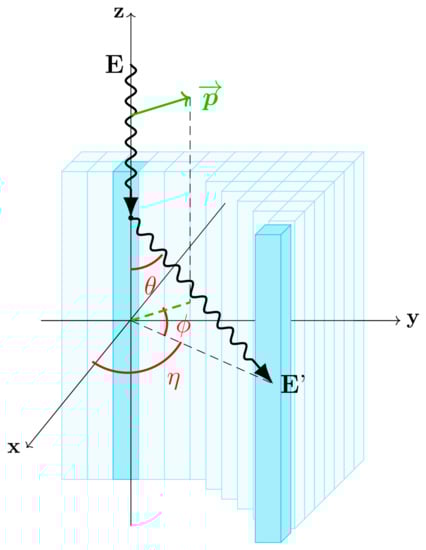
Figure 5.
Illustration of the measurement principle of a polarimeter using Compton scattering. The incoming -ray Compton scatters in one of the detector segments followed by a photo-absorption (or second Compton scattering) interaction in a different segment. Using the relative position of the two detector segments, the Compton scattering angle can be calculated from which, in turn, the polarization angle can be deduced.
At energies below approximately keV the cross section for photo-absorption dominates. Although no successful GRB polarization measurements have been performed using the photo-electric effect, the detection method has been successfully used recently to perform polarization measurements of the Crab Nebula in the 3–4.5 keV energy range using the PolarLight cubesat [195]. Several large-scale polarimeter ideas have been developed in the past, such as the Low-energy Polarimeter, which was part of the proposed POET mission, which was dedicated to GRBs [196]. Currently, several missions that use the same concept are currently under development [197,198]. In these X-ray polarimeters, the photo-absorption takes place in a thin gas detector. As the produced electron travels through the gas it releases secondary electrons as it ionizes the gas. These secondary electrons can be detected using finely segmented pixel detectors in order to track the path of the electron released in the photo-absorption interaction, allowing to reconstruct its emission angle.
Polarimetry in the pair-production regime is arguably the most challenging as the photon flux is low, and the detection method requires highly precise trackers capable of separating the tracks of the electron and the positron. In spectrometry, the low photon flux is often compensated by using large detectors with a high stopping power. For example, by combining tungsten layers with silicon detectors. Here, the silicon serves to measure the tracks while the tungsten is used to enforce pair production in the detector. However, the use of high Z (atomic number) materials, like tungsten, significantly increases multiple scattering of the electron and positron. Multiple scatterings quickly change the momentum of both products, thereby making it challenging to reconstruct their original emission direction. To overcome this issue, detectors that use silicon both for conversion and detection, have been proposed in the past such as PANGU [199]. Although technically possible, the large number of silicon detectors required to achieve a high sensitivity, with minimal structural material and a potential magnet, which helps to separate the electron–positron pair, make such detectors both costly and challenging to develop for space. A second option is to use gas-based detectors, such as in the HARPO design [200]. This detector, which was successfully tested on the ground [201], allows for precise tracking but has a low stopping power for the incoming -rays and therefore a low detection efficiency. This can be compensated with a large volume. However, as the gas volume obviously needs to be pressurized, producing and launching such an instrument for use in space is highly challenging. Despite these challenges, several projects that follow this design are still ongoing, such as the potential future space mission AdEPT [202], which aims to use a time projection chamber to measure polarization in the 5–200 energy range as well as the balloon borne SMILE missions [203].
Although no dedicated pair–production polarimeters are currently in orbit, it should be noted that both the Fermi-LAT [204] and the AMS-02 [205] instruments could, in theory, be used to perform polarization measurements in this energy range. For Fermi-LAT, which is a dedicated -ray spectrometer, consisting of silicon strip detectors combined with tungsten conversion layers, the aforementioned multiple scattering induced distortion is again a challenge [206]. The polarization capabilities of Fermi-LAT, which has detected many GRBs to this day, has been studied [206], but no results from actual data have been published to date. For AMS-02, which does not suffer from the use of tungsten layers and additionally contains a magnet which separates the pairs, measurements could be easier. However, as the instrument is designed as a charged particle detector, it remains non-optimized for this purpose, and so far no results have been published by this collaboration.
3.3. GRB Polarimeters
In this section, we aim to provide a summary of the different instruments that have performed GRB polarization to date. For a detailed overview of each individual measurement (up to 2016), the reader is referred to [186].
As mentioned earlier, all polarization measurements of the prompt GRB emission have been performed by making use of Compton scattering. While in the majority of cases the Compton scattering takes place in the detector, there is one exception. The attempts at performing polarization measurements with data from the BATSE detector made use of Compton scattering from the Earth’s atmosphere [207,208]. The BATSE detector consisted of several scintillator-based detectors and by itself had no capability to directly perform polarimetry [209]. Instead, it used several detectors pointing towards the Earth, each at different relative angles, to measure the relative intensity of photons scattering off different parts of the Earth’s atmosphere. As the probability for photons to scatter off the atmosphere towards different detectors depends on their polarization properties, such a measurement is possible for any detector with an Earth-facing sensitive surface. It does however require a highly detailed modelling of the Earth’s atmosphere, software capable of simulating the scattering effects properly, and detailed understanding of the detector response as well as the location and spectra of the GRB. The large number of sources for systematic errors resulted in inconclusive measurements of GRB 930131 [208]. Despite the initial lack of success, improvements have been made since then regarding Compton-scattering models in software such as Geant4 [210]. Furthermore, instruments such as Fermi-GBM have measured 1000 s of GRBs over the last decade, and similar studies using this data could prove to be successful in the future.
Systematic errors are a major issue not only for the creative polarization measurement solution used in BATSE but in all GRB polarization results published thus far from different instruments. It is especially important for measurements performed using detectors not originally designed to perform polarimetry such as RHESSI [211] and the SPI and IBIS detectors on board INTEGRAL. Both RHESSI and SPI make use of a segmented detector consisting of germanium detectors and thereby allow to study Compton scattering events by looking for coincident events between different detectors. The IBIS instrument [212] uses two separate sub-detectors instead, namely, the ISGRI detector consisting of 16384 CdTe detectors and the Pixellated Imaging CsI Telescope (PICsIT), an array of 4096 CsI scintillator detectors. Since, similar to RHESSI and SPI, IBIS was not originally designed to perform polarization measurements, the trigger logic in the instrument was not setup to keep coincidence events in the PICsIT or ISGRI alone. Rather, only coincidence events between the PICsIT and the ISGRI are kept, which although lowering the statistics for polarization measurements, still allows for such measurements [213].
Since all three instruments were not designed as polarimeters, one immediate downside of using them as such is the lack of sensitivity. A clear example of this is the non-optimized trigger logic of IBIS. In the case of RHESSI, different analyses of the same GRB [16] resulted in vastly different results, in part due to the difficulty in selecting valid coincident events between different germanium detector channels, again a result of a non-optimized online event selection. The relatively imprecise time measurement of each event prompted a large coincidence window to be set in one of the analyses, which resulted in chance coincidence events induced by different photons or background particles instead of the Compton scattering event [17,18]. If the instrument had been designed and tested on the ground as a polarimeter, the coincidence trigger logic and time measurement would likely have been optimized and event selection methods tested during the calibration phase.
The lack of on-ground calibration for polarization additionally makes verification of the detector response models difficult and prone to errors—for example, dead material around the detector can affect the polarization of the incoming flux when it interacts with it. While such issues are important in spectrometers as well, it can be argued that it is more important in a polarimeter. Imperfect modelling of certain detector channels for a spectral measurement can cause issues. However, if on average the channels are modelled correctly, having a few badly modelled channels will not greatly affect the final flux or spectral result, as over- and under-performing channels can cancel each other out. In a polarimeter it is the difference in the number of events between the detector channels that provides the final measurement and not, as in a simple spectrometer, the average of all the channels. For a polarimeter, however, one single over-performing detector channel would see a larger number of scattering events than expected, causing certain scattering angles to be favoured and thereby faking a polarization signal.
Similarly, dead material in front of the detector channels can easily obscure certain channels more than others causing a similar effect. Understanding all these issues during on-ground calibration is therefore crucial to reduce systematic errors. As a result of such difficulties, the polarization results published by the SPI collaboration clearly mention the possibility of significant systematic errors not taken into account in the analysis, which can affect the results [214,215].
In order to overcome such issues, more recent instruments, such as GAP [191] and POLAR [192], employ small coincidence windows and trigger logics optimized for polarization measurements. Most importantly, such detectors were calibrated prior to launch with polarized photons in different configurations, such as different photon energies and incoming angles [191,216,217]. GAP was the first dedicated GRB polarimeter. It made use of plastic scintillators used to detect Compton scattering photons together with 12 CsI scintillators used to detect the photon after scattering. The instrument flew for several years on the IKAROS solar sail mission during which it detected a few GRBs for which polarization measurements were possible. The POLAR detector also uses plastic scintillators, 1600 in total, to detect the Compton scattering interaction but uses the same scintillators to detect the secondary interaction. As a result, the instrument is less efficient for detecting the secondary interaction and has a poorer energy resolution. However, it allows for a larger scalable effective area as well as a larger field of view, which in the case of GAP is restricted by the CsI detectors that shield the plastic scintillators from a far off-axis source. The POLAR detector took data for six months on board the Tiangong-2 space laboratory, which resulted in the publication of 14 GRB polarization measurements [187].
Two other detectors, which although not fully optimized for polarimetry, were calibrated on the ground for such measurements. They are COSI [218] and the CZTI on Astrosat [194]. The balloon-borne COSI detector uses two layers of germanium double-sided strip detectors allowing for precise measurements of the interaction locations in the instrument. During its long-duration balloon flight in 2017, COSI saw one bright GRB for which a polarization measurement could be performed [219]. The CZT Imager on board the AstroSAT satellite uses, as the name suggests, a CZT semiconducter detector. As this detector is segmented, it allows to look for Compton scattering events. The detector was calibrated with polarized beams prior to launch to study the instrument response to on-axis sources [194]. AstroSAT CZTI has detected a large number of GRBs since its launch and has published polarization measurements of 13 of these to date while it continues to be operational.
4. Theoretical Models of Prompt GRB Polarization
The focus of this section is to present polarization predictions for the popular prompt GRB emission mechanisms, as highlighted in Section 2. Since GRBs are cosmological sources (of modest physical size in astrophysical standards), they remain spatially unresolved. Consequently, the measured polarization is the effective average value over the entire image of the burst on the plane of the sky. Therefore, the obtained polarization is affected by several effects, such as the intrinsic level of polarization at every point on the observed part of the outflow; the geometry of the outflow; i.e., the angular profile of the emissivity and bulk ; and the observer’s LOS. Even though GRBs are intrinsically very luminous, their large distances drastically reduce the observed flux, making them photon starved. This forces observers to integrate either over the entire pulse or large temporal segments of a given emission episode to increase the photon count. This causes additional averaging—time averaging over the instantaneous polarization from the whole source, which in many cases significantly evolves even within a single spike in the prompt GRB lightcurve.
Before presenting the model predictions for time-resolved polarization in Section 4.3, pulse-integrated polarization is discussed first. In the latter, any radial dependence of the flow properties is ignored for simplicity (but without affecting the accuracy of the calculation). As a result, pulse-integrated polarization ultimately amounts to integrating over a single pulse emitted at a fixed radius, where it is not important what that radius is as it does not enter any of the calculations.
Polarization is most conveniently expressed using the Stokes parameters , where I is the total intensity, Q and U are the polarized intensities that measure linear polarization, and V measures the level of circular polarization. In GRB prompt emission, the circular polarization is typically expected to be negligible compared to the linear polarization (; this is usually expected to hold also for the reverse shock and afterglow emission) and therefore we concentrated here on the linear polarization. The local linear polarization (all local quantities are shown with a “bar”) from a given fluid element on the emitting surface of the flow is given by e.g., [220]
where
and is the local polarization position angle (PA). When moving from the comoving frame of the jet to the observer frame, both the Stokes parameters and the direction of the polarization unit vector (, where and are the unit vectors in the comoving frame pointing along the observer’s LOS and direction of the local B-field, respectively) undergo a Lorentz transformation (e.g., Equation (13) of Gill et al. [24]). The degree of polarization (magnitude of the polarization vector), however, remains invariant (since ). The local polarization is different from the global one, (all global parameters are denoted without a bar), which is derived from the global Stokes parameters. It is the global polarization that is ultimately measured for a spatially unresolved source. For an incoherent radiation field, meaning the emission from the different fluid elements is not in phase, which is also true for most astrophysical sources, the Stokes parameters are additive. Therefore, each global Stokes parameter is obtained by integration of the corresponding local Stokes parameter over the image of the GRB jet on the plane of the sky, such that
where is the flux contributed by a given fluid element, of observed solid angle and area on the plane of the sky, and is the angular distance to the distant source. We worked with the Stokes parameters per unit frequency for convenience, such as the specific intensity . For simplicity, we ignored the radial structure of the outflow and assumed that the emission originates from an infinitely “thin shell”. This approximation is valid if the time-scale over which particles cool and contribute to the observed radiation is much smaller than the dynamical time. It implies that the emission region is a thin cooling layer of width (in the lab-frame) . In this approximation, the differential flux density from each fluid element radiating in the direction , i.e., the direction of the observer, when the radiating shell is at radius R (radial dependence included here for the general expression) can be expressed as [221]
where z and are the redshift and luminosity distance of the source, respectively; is the comoving spectral luminosity of the fluid element; and is its solid angle; with the polar angle measured from the LOS; and is the azimuthal angle around the LOS. The Doppler factor of the fluid element moving with velocity is given by (where the second expression holds for a radial outflow where ). In order to calculate the Stokes parameters using the differential flux density, the angular structure of the outflow needs to be specified, as was done next.
4.1. Polarization from Uniform Jets
In uniform axisymmetric jets, the comoving spectral luminosity, and the bulk- do not vary with polar angle measured from the jet axis, e.g., in a top-hat jet,
It is further assumed that , , , and the spectrum (assumed here to be a power law) remain constant with the radius during emission of the prompt GRB (while can vary with the radius). Since the emission arises in an ultrarelativistic jet (), it is strongly beamed along the direction of motion primarily into a cone of angular size . Consequently, most of the observed radiation arrives from angles around the LOS. If the LOS intersects the jet surface and is more than a beaming cone away from the edge of the jet, i.e., if or equivalently if where , then the observer remains unaware of the jet’s edge (however, see Section 4.3), and the emission can be approximated as if arising from a spherical flow. In this instance, after averaging over the GRB image on the plane of the sky, a finite net polarization will only be obtained if the direction of polarization is not axisymmetric around the LOS. Hence, it becomes necessary to break this symmetry in order to obtain any net polarization. This naturally happens if the LOS lies near the edge of the jet. Therefore, in such cases a special alignment between the flow direction and the observer is needed. This and other effects that break the symmetry and yield finite net polarization are highlighted below.
4.1.1. Synchrotron Emission from Different Magnetic Field Structures
Synchrotron emission is generally partially linearly polarized. The local polarization emerging from a given point on the outflow depends on the geometry of the local B-field and distribution of the emitting electrons, both in energy, , and pitch angle, , where is a unit vector pointing in the direction of the electron velocity. In the case of power-law electrons, with distribution for , and with isotropic velocity distribution so that all pitch-angles are sampled during the emission, the maximum local polarization for a locally ordered B-field depends on the spectrum [108,220]
Here is the local spectral index, and is the effective power-law index of the electron distribution. Since the local value of (and therefore also of ) smoothly varies with , the maximum polarization, , also varies smoothly with across the spectral breaks of the synchrotron spectrum. The asymptotic spectral index is different for different power-law segments (PLSs) of the well-studied [87,88] broken power-law synchrotron spectrum. We have , , and for (fast cooling); , and for (slow cooling); , and for (either slow or fast cooling). For , there is no since emission in this PLS arises from all cooling electrons that are emitting below their typical (optically thin) synchrotron frequency. In this case, and , the lowest local polarization obtained from synchrotron emission. On the other hand, shock-acceleration theory suggests that , which means that the maximum local polarization in synchrotron is limited to .
When the magnetic fields are tangled or switch direction on angular scales , e.g., in the case, the local polarization must be averaged over different B-field orientations. This has been calculated for an infinitely thin ultrarelativistic shell, while assuming , for a tangled B-field [109,222,223]
where is the polar angle measured from the LOS in the comoving frame (this holds for a radial flow and more generally ). The level of anisotropy of the B-field is quantified by the parameter , which represents the ratio of the average energy densities in the two field orientations. The factor of two simply reflects the two independent directions of the component, such that for a field that is isotropic in three dimensions.
The polarization map over the GRB image on the plane of the sky is shown in Figure 6 for different B-field structures (for ). Only the area contained within the beaming cone, shown by the red circle, contributes dominantly to the emission. Outside of it, the intensity is strongly suppressed by relativistic beaming, which scales as a power of the Doppler factor. This effect is reflected by the decrease with the angle from the LOS (shown by the red “+” symbol) in the size of the black arrows, which correspond to the magnitude of the polarized intensity. When the jet possesses axial symmetry (and for synchrotron emission the same requirement holds also for the global magnetic field structure), then the image and polarization map are symmetric to reflection along the line connecting the jet symmetry axis to the LOS. Therefore, it is natural to choose a reference direction for measuring the local PA either along this line or transverse to it (in the figure, as well as are measured from the latter, i.e., the horizontal direction). For such a choice, i.e., the local Stokes parameter vanishes when integrated over the GRB jet image, and therefore the global polarized intensity is entirely given by Stokes Q, i.e., the integration of over the image, where the sign of for each fluid element depends on the local PA . The different B-field configurations produce completely different polarization maps, with distinct patterns of regions contributing predominantly either to polarization along the line connecting the jet symmetry axis to the LOS (orange–yellow, with local polarization ) or transverse to it (blue–white, with local polarization ), as shown by the color map. When averaged over the entire GRB image, these are the only two directions of polarization that can be obtained in an axisymmetric flow in which the magnetic field also possesses axial symmetry about the jet axis, such that it would represent a change of in the PA when the direction of polarization switches from one to the other.
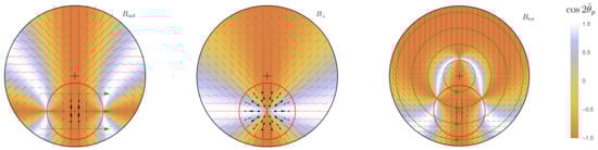
Figure 6.
Polarization map for different B-field configurations shown on the surface of a top-hat jet (for ). The jet symmetry axis marked with a black “+” symbol and the observer’s LOS is marked with a red “+” symbol. The region where the LOS is within the beaming cone of the local emission (i.e., from which the radiation is beamed towards us) is within the red circle, outside of which the the polarized intensity (as shown by the size of the black arrows) declines sharply. The red line segments show the direction and polarized intensity, now without the de-beaming suppression. Green lines show the orientation of the magnetic field lines (in the cases and where it is locally ordered). The color map shows , with being the local polarization angle measured counter-clockwise from the horizontal axis, which corresponds to the level at which each point is polarized either along the line connecting the LOS with the jet symmetry axis (orange-yellow dominated) or transverse to it (blue-white dominated).
An example of a B-field configuration that does not possess such axial symmetry is . When is not oriented along the line connecting the jet symmetry axis to the LOS or perpendicular to it, then this breaks the symmetry of the image polarization map, thereby enabling other directions of net global polarization to occur, and the corresponding PA can vary continuously with a finite [109].
The level of net polarization after averaging over the GRB image depends on the level of symmetry of the polarization map around the LOS. In the case of , and likewise for , the polarization map is symmetric around the LOS and therefore averaging over the GRB image would yield zero net polarization () due to complete cancellation for a spherical flow (or well within a top-hat jet, ). This symmetry is naturally broken in and where the local B-field is ordered and provides a particular direction (transverse to the local B-field direction and to the propagation direction of the photon) along which the polarization vector aligns. Another way to break the symmetry is by having the LOS close to the edge of the jet, with (), so that some part of the beaming cone lies outside of the jet surface. The missing emission, which would otherwise contribute towards cancellation, leads to only partial cancellation and yields a net finite polarization, . The sign of net polarization is decided by whichever region, either blue–white or orange–yellow, makes the dominant contribution to the polarized flux. In Figure 6, for both and , whereas for .
Pulse-integrated polarization as a function of q is shown in Figure 7 for different B-field configurations and different , where the latter describes how wide or narrow the jet aperture is compared to the beaming cone. The polarization curves look very different for the three different field configurations, but there are some features that are worth pointing out. The polarization vanishes when the observer is looking down the jet axis, i.e., when (), in all cases due to complete cancellation (such a cancellation would not occur for , which is not shown in Figure 7). For , polarization grows rapidly for (for which it saturates at ) but slowly for both and . It reaches a local maxima when the LOS is close to the jet edge, i.e., as before, when , and declines sharply for and when the LOS exceeds one beaming cone outside of the jet, i.e., (). The case yields a different behavior where becomes maximal when the jet is viewed from outside its edge. In all cases, when the fluence drops off very sharply for a top-hat jet. So, even though a large is expected for , it will be challenging to detect. Finally, a change in the PA by occurs when () for and , at which point .
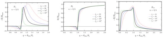
Figure 7.
Pulse-integrated polarization of synchrotron emission for different B-field configurations shown for different LOSs (q) and size of the beaming cone w.r.t to the jet aperture (). The spectral index was fixed to , where a larger produced a larger . Figure adapted from [24] but originally produced in [108].
It is clear from Figure 7 that only the case, an ordered field scenario, yields high levels of polarization when the LOS passes within the aperture of the jet. Since all distant GRBs must be viewed with , otherwise they will be too dim to detect, a measurement of will strongly indicate the presence of an ordered field component. On the other hand, if the B-field configuration is more like or , then most GRBs will show negligible polarization.
4.1.2. Photospheric Emission from a Uniform Jet
A photospheric spectral component can arise and even dominate the spectral peak in scenarios where energy is dissipated below the photosphere. At the photosphere, radiation decouples from matter and is able to stream freely towards the observer. However, in a matter-dominated flow in which the baryon rest mass energy density, , is much larger than that of the radiation field, , the radiation field becomes highly anisotropic at the photosphere [55]. At the last scattering surface, this produces significant local polarization at each point of the observed part of the flow. Nevertheless, upon averaging over the GRB image the net polarization is expected to be negligible in an axisymmetric uniform flow since there is no preferred direction for the polarization vector. To obtain finite net polarization, an inhomogeneous outflow with gradients in bulk- (and to a lesser extent in comoving emissivity ) across the beaming cone are needed. This scenario is discussed in Section 4.2.
Alternatively, if the flow is radiation-dominated, i.e., , as shown by Beloborodov [55], the comoving angular distribution of the radiation field is preserved in the ultrarelativistic limit as the flow goes from being optically thick to thin. This occurs due to the fact that radiation always tries to push the plasma to an equilibrium Lorentz frame in which the radiative force on the plasma vanishes. As a result, the radiation field accelerates the plasma to a bulk LF , which is a special Lorentz frame in which the (comoving) direction of freely streaming photons w.r.t the local radial direction remains unchanged in between successive scatterings. This means that an isotropic radiation field remains isotropic. Since scattering an isotropic radiation field only produces another isotropic field, the flow behaves (to leading order) as if no scatterings took place. Since the radiation field was necessarily isotropic when the flow was optically thick at smaller radii, leading to zero local polarization, it must yield the same (to leading order) when it becomes optically thin, as shown below.
The radiation field is able to accelerate the flow to only if and while the matter maintains a small lag, , which is initially (where these LFs are of the respective local center of momentum frames) corresponding to a relative velocity , but it gradually increases until it eventually becomes comparable to the two near the saturation radius where (for ), the point beyond which matter stops accelerating and starts coasting, while the scaling remain valid as the radiation-free streams in increasingly more radial directions. In a steady radiation-dominated spherical flow the comoving radiation energy density scales as , and the rest mass energy density of the particles scale as , where is the comoving volume. This yields , which for gives and . This further yields so that and . Near the comoving radiation anisotropy becomes significant () and therefore so does the polarization of the radiation scattered at , but this is only a fraction of the photons, and therefore the overall local (i.e., from a particular fluid element) polarization is of the same order, i.e., very small.
4.1.3. Compton Drag
Inverse-Compton scattering of anisotropic radiation yields high levels of polarization for the scattered radiation field with . This is very different from Comptonization since the polarization vector of the scattered photon can now be aligned with a particular direction, which is transverse to the plane containing the wave vectors, and , of the incoming and scattered photons, respectively, in the rest frame of the electron (hence the double primes). If the scattering angle is , then Thomson scattering of radiation imparts local polarization
to the outgoing photon. Indeed, if , then . Here it was assumed that the electrons are cold and therefore their rest frame is the fluid frame () that is moving with velocity , and if it is moving everywhere in the radial direction (), then . In general, the local polarization depends on the angle between the wave vector of the incoming photon and the velocity vector of the electron. If the electrons have a finite internal energy density, which means that they have a velocity distribution, then the local polarization is obtained by performing a weighted integral over all—see [224] for details.
The expected polarization when assuming cold electrons in the comoving frame of an ultrarelativistic top-hat jet is shown in Figure 8. The polarization curves are very similar to that obtained for synchrotron emission for the field configuration, but for Compton drag the normalization is (nearly exactly) higher by as given by Equation (10). Similar results were first obtained by Lazzati et al. [134] for narrower jets with where they showed that when very high polarization with can be obtained with Compton drag.
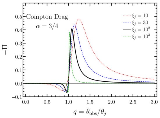
Figure 8.
Pulse-integrated polarization of prompt GRB radiation generated by the Compton drag mechanism. The electrons were assumed to be cold in the comoving frame. Figure adapted from [24], but also see [134] for results for a narrower top-hat jet.
4.2. Polarization from Structured Jets
The angular structure of the relativistic jet in GRBs becomes particularly important for relatively nearby events, e.g., GRB170817A ( Mpc), which can be detected with the current cadre of instruments when the observer is relatively far off-axis and the emission is dim. For distant GRBs, as mentioned earlier, it is challenging to detect emission from significantly off-axis jets. Still, there will be some events in which the LOS is just outside the quasi-uniform core that may not be sharp, as found otherwise in a top-hat jet, but instead be smoother. Then, it becomes important to model the angular structure and compare polarization measurements with accurate theoretical models.
The first level of correction for an idealized top-hat jet model is the consideration of smooth wings of comoving spectral luminosity while the bulk- remains uniform [225]. Like the top-hat jet, for (), but outside of this uniform core the spectral luminosity can have either exponential or power-law wings:
Here again it is assumed that , , , and the spectrum do not have any radial dependence.
In a more realistic structured jet the core is no longer uniform. Instead, the spectral luminosity as well as the bulk- depend on polar angle . In general, the properties of the flow can also depend on the azimuthal angle , but here the discussion makes the simplifying and physically reasonable assumption of axisymmetric jets. Two different types of structured jets are considered here:
Here, and are the core spectral luminosity and bulk- at .
4.2.1. Synchrotron Emission from Structured Jets
The polarization curves for a smooth top-hat jet are presented in Figure 9 for different B-field configurations as well as for different levels of smoothness of the edges. The behavior is similar for , but significant differences between the top-hat jet case appear for . Now that the spectral luminosity does not fall off so sharply for off-axis observers in the latter case, there is always some emission beamed along the LOS. For B-field configurations that show a larger degree of symmetry of the direction of polarization vectors around the LOS (e.g., and ), the net polarization starts to decline as the edges of the jet are made smoother. This occurs due to the increase in symmetry that was broken sharply in the top-hat jet. A completely opposite behavior is seen in ordered B-field configurations, where the polarization increases with increasing smoothness. This arises since for a very sharp edge the observed flux is dominated by the core and once most of it has a similar weight (i.e., beaming and Doppler factor) then a significant amount of canceling occurs, while for a very smooth or gradual edge the flux is dominated by the region near the line of sight where the B-field is ordered, resulting in very little averaging out of the polarization.
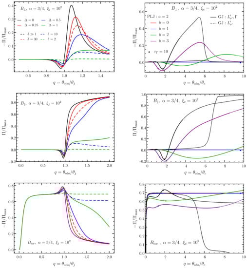
Figure 9.
(Left) Pulse-integrated polarization for smooth jets with uniform core and exponential or power-law wings in spectral luminosity while the bulk- remains uniform. The edges of the uniform jet become smoother with increasing (decreasing) () for exponential (power law) wings. (Right) Polarization curves for structured jets. Two cases for the Gaussian jet (GJ) are shown, where in one both and vary with and in the other is kept uniform. For the power-law jet (PLJ), the power-law index for is fixed (), but that for the bulk- (b) is varied. The curve for is mostly overlapped by that of . The dotted lines show the polarization curves for viewing angles at which the fluence has declined to values smaller than of that expected at . The thick dots mark critical viewing angles beyond which the emission region becomes too compact to -annihilation, causing the emission to be optically thick to Thomson scattering of the produced -pairs. Figure adapted from [24] and some results for the smoothed top-hat jets were first presented in [225].
The right column of Figure 9 shows the polarization curves for structured jets. When compared with polarization curves from top-hat jets or even smooth top-hat jets, these are broadly similar. Note that the smooth top-hat jet (left panel of Figure 9) is broadly similar in structure to (, ) structured jet (right panel), where both show similar polarization behavior, and therefore a smooth top-hat jet can also be considered a structured jet. In all cases, the curves are now stretched towards larger viewing angles. This means that appreciable polarization can now be measured when the LOS falls outside of the brighter core. In addition to that, the drop in fluence for viewing angles outside of the core is not so severe, as was found for the top-hat jet. Therefore, depending on the exact angular profile, off-axis observers with few to several can still detect the GRB and measure high levels of polarization. This is demonstrated in Figure 9 using a dotted line where the solid to dotted line transition occurs when the off-axis () to on-axis () fluence ratio has dropped to . Nevertheless, there are additional constraints on the detectability of such off-axis bursts. For example, when the bulk- is non-uniform and declines with , the viewing angle out to which the prompt emission can be observed may be limited by compactness e.g., [24,145,226]. This is shown using a thick dot in the figure beyond which the Thomson optical depth of the -pairs () produced due to -annihilation becomes greater than 10. As a result, the polarization is rather limited to for and , but it can be much higher for the ordered field in .
4.2.2. Photospheric Emission from Structured Jets
Photospheric emission yields negligible polarization in a uniform jet unless the viewing angle is less than one beaming cone away from the edge of the jet, i.e., . One way to obtain finite net polarization is by having a structured jet (see Figure 10). This was initially demonstrated in Monte Carlo (MC) simulations of photospheric emission emerging from axisymmetric relativistic outflows [56,57] that featured sheared layers outside of the uniform core with gradients in bulk- as a function of the polar angle . It was shown that narrow jets with and steep gradients in bulk- with for (some works use the symbol instead of to refer to the half-opening angle of the uniform core) and can yield polarization for . A more realistic scenario would have in which case is expected. A similar conclusion is reached by carrying out a radial integration of the radiation transfer equations for the Stokes parameters in a steady flow having angular structure in the comoving emissivity and bulk- [24]. The results of this work are shown in the bottom-left panel of Figure 10, and even here it was realized that steep gradients in the bulk- profile are required to achieve significant polarization with .
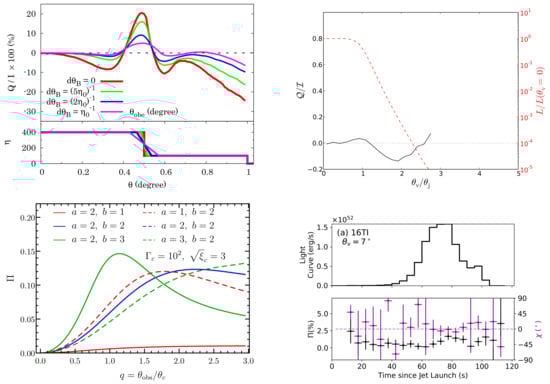
Figure 10.
Polarization from non-dissipative photospheric emission model in a structured jet. (Top-left) Polarization from the Monte Carlo (MC) simulation of Ito et al. [56] shown for different viewing angles and different gradients in bulk- (here ). (Top-right) MC simulation results from Lundman et al. [57] featuring a uniform core with half-opening angle and power-law shear () layer in bulk-. The off-axis spectral luminosity normalized by the on-axis value (viewing angle ) is shown with dashed red line. (Bottom-left) Polarization of photospheric emission from a structured jet obtained from semi-analytic radiation transfer calculation of Gill et al. [177] that features angular structure in both the comoving emissivity (, see Equation (10)) and bulk- () with where is the core angle. The solid lines fix and dotted lines set to disentangle the effect of the two profiles. (Bottom-right) Polarization derived from a MC simulation with outflow properties obtained from a 2D special relativistic hydrodynamic simulation of a jet launched inside a Wolf–Rayet star (from Parsotan et al. [58]). The top-panel shows the lightcurve and the bottom panel shows the temporal evolution of and position angle .
A more realistic scenario was explored in Parsotan et al. [58] who carried out two-dimensional (2D) special relativistic hydrodynamic simulations of a jet launched inside a Wolf Rayet star. The flow dynamics and angular structure thus obtained from the simulation were then used with a MC code to obtain the polarization of photospheric emission at the last scattering surface. The results are shown in the bottom-right panel of Figure 10 that shows the lightcurve and temporal evolution of the polarization and PA, with the conclusion that and PA remained steady within the uncertainties. In other cases, where the outflow showed more structure, a slightly larger time-resolved polarization of and time-variable PA was obtained.
4.3. Temporal Evolution of Polarization
The earlier sections only discuss the pulse-integrated polarization, which is relevant for most GRBs that are not bright enough to be able to yield any time-resolved polarimetric results. However, with the upcoming more sensitive gamma-ray polarimeters in the next decade time-resolved polarimetry of prompt GRB emission will become possible. Therefore, in anticipation of such a development, it is prudent to also construct accurate theoretical model predictions to compare with time-resolved polarization measurements.
When discussing time-resolved polarization it becomes important to include the radial dependence of the flow properties, which were ignored for the pulse-integrated discussion. We first describe a simple and very general pulse model of an accelerating, coasting, or decelerating flow (see, e.g., [227,228]), which is then used to calculate the time-resolved polarization. Consider a thin ultra-relativistic shell that starts to emit prompt GRB photons at radius . The emission continues over a radial extent and terminates at . During this time, the comoving spectrum, with spectral peak frequency , and spectral luminosity evolve as a power law with radius,
where and are the normalizations. The factor describes the angular profile of where it is normalized to unity at the jet-symmetry axis with , for a uniform spherical flow and for a top-hat jet with being the Heaviside function and the jet half-opening angle. The comoving spectrum is described by the function , which is considered here to be the Band function, where . The dynamics of the thin shell are given by the radial profile of the bulk-, such that where . The shell is coasting when and accelerating (decelerating) for (. Once the power law indices a and d for are provided, one has complete information of the temporal evolution of the pulse. These indices depend on the details of the underlying prompt GRB model, e.g., on the composition and dissipation mechanism. If the prompt GRB spectrum is assumed to be of synchrotron origin, then it can be shown [84] that for a KED flow, where energy is dissipated at internal shocks (), and . Alternatively, if the flow is PFD with a striped wind B-field structure and energy is dissipated due to magnetic reconnection, which also accelerates the flow with , then it is found that and .
The pulse profile and temporal evolution of polarization for a KED flow coasting at is shown in Figure 11 for an ordered B-field (). The different curves are shown for observed frequency , which is a fraction of the peak frequency of the first photons emitted along the LOS at radius . The apparent arrival time of these first photons is given by , which is the characteristic radial delay time between the shell to arrive at radius and the hypothetical photon that was emitted by the engine at the same time as the shell. For , this is also the angular time over which radiation from within the beaming cone around the LOS arrives at the observer. Depending on , the pulse profile changes and shows a peak at different times with the latest peak occurring at , the arrival time of last photons emitted along the LOS from radius . At , the flux density declines rapidly, and the pulse becomes dominated by high-latitude emission that originates from outside of the beaming cone, i.e., from angles larger than from the LOS.
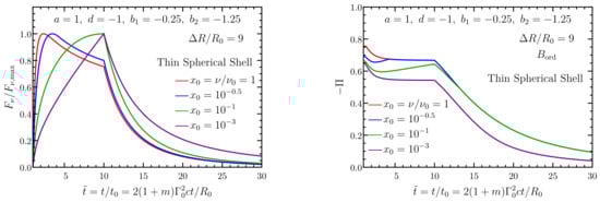
Figure 11.
Pulse profile (left) and temporal evolution of polarization (right) for a coasting () ultrarelativistic () thin spherical shell with an ordered field (). Here, energy is dissipated in internal shocks in a KED flow and the emission is synchrotron, which is modeled using a Band function with asymptotic spectral indices and . The shell starts to radiate at and terminates at radius . The comoving spectral luminosity and spectral peak evolve as a power law in radius with indices a and d, respectively (see Equation (16)). The different curves show the trend at the observed frequency where is the -peak frequency of the first photons emitted along the observer’s LOS from radius , which then arrive at the apparent time . The emission is assumed to have a Band function spectrum with asymptotic power-law spectral indices and below and above the spectral peak energy, respectively. Figure adapted from [84].
The polarization curves show maximal polarization initially, corresponding to depending on the local value of the spectral index for the Band function as set by . For , the polarization first declines and then saturates, which reflects the averaging of local polarization over the beaming cone as seen on the plane of the sky, which tends to yield a net polarization lower than . For , like the pulse profile, the polarization also declines rapidly when high-latitude emission becomes dominant. The polarization curves at different merge at , the crossing time of the break frequency across the observed frequency as the entire spectrum drifts towards softer energies over time. The merging of the polarization curves occurs due to the fact that after time all photons at the observed frequency are harder than the Band-function break frequency beyond which the Band function features a strict power law with a given spectral index. Therefore, the level of polarization for all photons sampling the power law is also the same as dictated by .
The polarization is not always maximal at the start of the pulse if the magnetic field is not ordered. This is demonstrated in Figure 12 that shows the pulse profile and temporal evolution of synchrotron polarization for different B-field configurations in a top-hat jet. As argued earlier, in B-field configurations, e.g., and , that produce axisymmetric polarization maps around the LOS the net polarization vanishes. This symmetry is only broken when the observer becomes aware of the jet edge, e.g., in a top-hat jet. It is at that instant the magnitude of polarization begins to grow above zero. The polarization curves for the three B-field configurations also show a change in the PA by when the curves cross zero. Interestingly, this happens more than once for . The reason for this can be understood from the polarization maps shown in Figure 6 where the change in the PA occurs when the net polarization begins to be dominated by emission polarized along the line connecting the jet symmetry axis and the observer’s LOS over that polarized in the transverse direction or vice versa. At late times, the observed emission vanishes after the arrival time of the last photons from the edge of the jet furthest from the LOS. Since the flux declines very rapidly at , the changes in the PA are challenging to detect in practice.
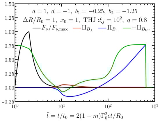
Figure 12.
Pulse profile (black) and temporal evolution of synchrotron polarization in a top-hat jet (THJ, with and ) for different B-field configurations. See caption of Figure 11 for explanation of different symbols and parameters. Figure adapted from [84].
4.4. Polarization from Multiple Overlapping Pulses
Since GRBs are generally photon-starved, the only hope of obtaining a statistically significant polarization measurement often relies on integrating over broad segments of the prompt GRB lightcurve. Due to the highly variable nature of the prompt GRB emission, a given emission episode consists of multiple overlapping pulses. The properties of the emission region, e.g., bulk-, B-field configuration, can change between different pulses and improper accounting of these changes in calculating the time-integrated polarization can lead to erroneous results.
In the simplest scenario, multiple pulses are produced by distinct patches or mini-jets within the observed region of size of the outflow surface. These patches can be permeated by an ordered B-field the orientation of which is also mutually distinct among the different patches. A broadly similar B-field structure can also be obtained in both internal and external shocks due to macroscopic turbulence excited by, e.g., the Richtmyer–Meshkov instability, which arises in the interaction of shocks and upstream density inhomogeneities [68,69,70,229]. In the case of mini-jets, the bulk- of the different jets can also be different by a factor of order unity, which will affect the size of the individual beaming cones. Since the Stokes parameters are additive for incoherent emission the time-integrated net polarization of incoherent patches (in the visible region of angular size around the line of sight) is obtained from [63] (where the motivation was afterglow emission from a shock-generated field rather than incoherent patches or mini-jets).
The net polarization is significantly reduced for increasingly large numbers of patches due to the fact that the PA are randomly oriented, and when added together some cancellation occurs. This essentially represents a random walk for the polarized intensity Q while the total intensity adds up coherently. When multiple time-integrated segments of an emission episode are compared, the net polarization and PA will vary between them (the latter is possible as this is a non-axisymmetric global configuration). Alternatively, instead of ordered B-field patches, one can have a shock-produced B-field (e.g., ) with a patchy shell or mini-jets that give different weights to different parts of the image and thereby produce a net polarization (see, e.g., [109,230]).
Another scenario that is worth considering is when multiple overlapping pulses are produced by episodic energization of the emission region, e.g., in the collision of multiple shells in the internal shock scenario where the ejection time of subsequent shells is different, such that the ejection time of the shell in the engine frame is . The onset time of each pulse is then given by . The scenario of multiple pulses from a smooth top-hat jet is demonstrated in Figure 13 using simplifying assumptions, where all pulses have the same and (so that the radial delay time for emission arising from different pulses is the same) and radial extent . In this case, the onset times of pulses is simply dictated by the different ejection times of the shells. The left panel shows the pulse profile, and the right panel shows the polarization calculated for the field. Time-resolved polarization obtained from multiple temporal segments, where the emission episode is divided into one, two, or three equal duration segments, is shown to demonstrate the different levels of polarization obtained when using the multi-pulse or the single-pulse model. Therefore, when the emission consists of multiple overlapping pulses, it is important to compare the measurement with model predictions that account for multiple pulses.
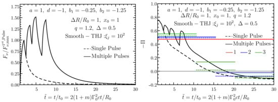
Figure 13.
(Left) Pulse profile of multiple overlapping pulses in an emission episode, shown here for a KED smooth top-hat jet. A single pulse is also shown for comparison. (Right) Temporal evolution of the polarization for a toroidal magnetic field () shown for both the single pulse and multiple pulses. Temporal segments over which polarization is obtained are calculated by dividing the pulse into one (red), two (blue), or three (green) part(s). See the caption of Figure 11 for explanation of different symbols. Figure adapted from [84].
4.5. Most Likely Polarization Measurement
As demonstrated in earlier sections, the prompt GRB polarization depends on (i) the underlying radiation mechanism, (ii) B-field structure (for synchrotron emission), (iii) bulk LF (top-hat jet) or (structured jet), (iv) (top-hat jet) or (structured jet), (v) viewing angle , and (vi) angular structure, e.g., power-law indices a and b for a power-law structured jet (see Section 4.2). Due to variations in these parameters the polarization can vary between different pulses within the same GRB as well as between different GRBs. For an ultrarelativistic flow, three basic quantities naturally arise that affect the polarization, namely, (a) the normalized jet/core half-opening angle: (top-hat jet) or (structure jet), (b) the normalized viewing angle: (top-hat jet) or (structured jet), and (c) the normalized viewing-angle dependent fluence: (top-hat jet) or (structure jet), which is the ratio of the off-axis to on-axis isotropic-equivalent radiated energy or equivalently the fluence.
For different pulses emitted by the same GRB, it is natural to expect a considerable change in (iii), while the other parameters are likely to remain more or less fixed. In, e.g., a top-hat jet, this will change the parameter , and, for a given distribution of between several pulses, the total polarization, after integrating over multiple pulses, will be different from that obtained for a single pulse. When adding up the Stokes parameters of different pulses, an appropriate relative weight using, e.g., (or more precisely the relative expected number of photons that will be detected), should be applied.
When comparing emission from different GRBs all of the above-mentioned quantities can in principle vary (or at least there is no strong evidence against this in the observed sample of GRBs). In this case, the fluence ratio is important in determining (i) whether for a given (top-hat jet) or (structured jet) the pulse will be bright enough to be observed by a given detector and (ii) for a given GRB out to which viewing angle it will be fluent enough for performing polarization measurements. For a top-hat jet, the fluence is strongly suppressed due to Doppler de-beaming when , whereas, for a structured jet, the suppression in fluence is not as severe and emission from few to several can be detected if it is not suppressed due to compactness, as discussed earlier.
A distribution of polarization for a given radiation mechanism, while accounting for variations in the aforementioned quantities between different pulses from the same source and different GRBs, and its comparison with actual measurements can be used to answer some of the key questions of GRB physics. Such a distribution obtained from a Monte Carlo simulation (see [24] for more details) is shown in Figure 14 for a power-law jet and for different radiation mechanisms as well as different B-field configurations. As expected, the field being ordered yields the highest polarization with . Therefore, if GRB jets feature a large-scale toroidal field, then most GRBs that are emitting synchrotron radiation will show . For the other two B-field configurations, and , the expected polarization is small with , and one is most likely to find GRBs with negligible polarization. The same conclusion can be drawn for the Compton drag and photospheric radiation mechanisms. The polarization in the photospheric emission model can be when the flow features a much steeper bulk- angular profile with few (see Figure 14 of [24] for more details). When comparing with observations, some of which have at least detection significance, no firm conclusions can be drawn at this point. Measurements made by IKAROS-GAP and AstroSat-CZTI find highly polarized GRBs with , although with large error bars. On the other hand, the POLAR data appear to indicate that GRBs are more likely to have significantly smaller polarization with most of their sample consistent with unpolarized sources. The apparent discord between the results of these works not only highlights the challenges involved in obtaining a statistically significant polarization measurement but also calls for the need to build more sensitive detectors.
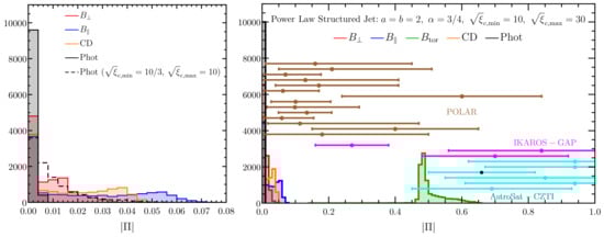
Figure 14.
(Right): Distribution of polarization from synchrotron emission for different B-field configurations, Compton drag (CD), as well as photospheric (Phot) emission in a power-law-structured jet obtained from a Monte Carlo simulation (with samples). Measured polarizations with error bars from different instruments are shown for comparison. The measurement of () from [231] obtained using AstroSat-CZTI is shown with a black dot with cyan error bars. Figure adapted from [24] where more details can be found. (Left): Zoomed-in version of the figure showing the several overlapping distributions for clarity (with a bin size smaller by a factor of ).
4.6. Energy Dependence of Polarization
Polarization is energy dependent. This can be easily seen in emission mechanisms where the local polarization depends on the spectral index, e.g., in optically thin synchrotron radiation (see Equation (10)). The energy-dependent spectro-polarimetric evolution in this case is shown in the left panel of Figure 15; temporal evolution of polarization at a given energy and the pulse profile for the same case was shown earlier in Figure 12. The polarization is sensitive to the local spectral index, which, for a Band-like spectrum, changes near the spectral peak and asymptotes far away from it.
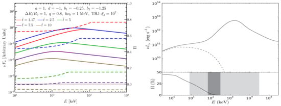
Figure 15.
(Left): Temporal evolution of the Band-like spectrum (solid lines; left y-axis) and the corresponding polarization (dashed lines; right y-axis) from synchrotron emission with a field for a KED top-hat jet (THJ) with and , and . The different colours correspond to different normalized apparent times where is the arrival time of the initial photons emitted from radius along the LOS. The peak frequency of the spectrum at this time is given by . (Right): Multi-component GRB spectrum and its energy-resolved polarization. While the photospheric component dominates both spectral peak and at higher energies, the low-energy spectrum is produced by synchrotron emission. As a result, the polarization grows towards lower energies as the fraction of synchrotron photon grows. The light and dark shaded regions correspond to the energy ranges of Fermi GBM (NaI + BGO detectors, (8–30 MeV), and GAP (70–300 keV), respectively. Figure from [232].
Energy-dependent polarization is possible also in emission mechanisms where the local polarization is independent of energy, such as Compton drag in the Thomson regime (where the energy-independent Equation (12) holds). A featureless power-law spectrum will have no energy dependence, but the energy-independent polarization would still depend on the spectral power-law index, . This occurs since different -values give different weights to different parts of the image between which the Doppler factor varies such that the same observed frequency corresponds to different comoving frequencies. For a non-featureless spectrum, the same effect can cause energy dependence in the polarization, e.g., for a Band spectrum, the relative weights of different parts of the image (and therefore also the polarization) will depend on the initial location of the observed frequency relative to the peak frequency along the LOS (i.e., on ).
Alternatively, if multiple spectral components from different radiation mechanisms having different levels of polarization contribute to the observed spectrum, the polarization of the total spectrum will change with energy. This is expected in some photospheric emission models [232] that posit that the spectral peak is dominated by the quasi-thermal photospheric component while the low and/or high energy wings may come from synchrotron emission (see, e.g., Figure 2 and discussion in Section 2.3.3). The right panel of Figure 15 presents such a case, where the polarization grows with decreasing energy owing to the dominance of flux by the synchrotron component. Near the spectral peak, the polarization vanishes. In this way, energy-resolved polarization measurements can be invaluable in understanding the GRB radiation mechanism.
5. Observations
5.1. Time-Integrated Polarization Measurements
To date, the -ray polarization of a total of 31 GRBs has been published. For several GRBs, different analyses have been published, either by different groups using the same data or, in one case, using data from two different instruments. The time- and energy-integrated polarization parameters from these measurements are shown in Table 1, together with the energy range in which they were performed. It is important to note that the energy ranges mentioned here are those stated in the respective publications but that their definitions differ between experiments. The energy ranges stated by SPI for example come from an event selection based on the deposited energy, whereas, for POLAR, which cannot perform measurements of the incoming photon energy directly, the stated range is based on the energy-dependent effective area to polarization.

Table 1.
The list of all GRBs for which a measurement has been published to date. For GRB 160821A, several analyses were published by members of the AstroSAT collaboration. For this GRB, a time-resolved analysis found high levels of polarization with varying PA as well.
As can be seen from Table 1, especially for the earliest measurements, at the bottom of the table, the results indicate typically high levels of polarization, although, as explained earlier, this can in some cases be attributed to an error in the analysis. Additionally, publications of GRB polarization measurements have focused on those measurements for which a non-zero PD was found. At least several GRB measurements exist, such as some detected by GAP, for which the PD was found to be compatible with ; however, these were not published but only presented at conferences (https://ttt.astro.su.se/groups/head/cost14/talks/Yonetoku.pdf talk accessed on 25 August 2014). This causes an additional bias towards higher PD values found in the list.
In recent years, data from GAP, POLAR, and Astrosat CZTI have significantly increased the number of measurements; however, the measured PD shows a large range between the different instruments. POLAR finds results that are mostly compatible with a low or unpolarized flux, whereas Astrosat CZTI reports high levels of polarization in [188], with best fitting PD for 10 out of the 11 GRBs exceeding . Although in numerical form only an upper limit is provided for some of these GRBs by Astrosat CZTI (which are the numbers reported in Table 1) mthe contour plots for these GRBs in Figure 13 of [188] indicate that high levels of PD are favoured for all. In most cases, the best fitting PD is close to the upper limit. The only exception is 160623A where a best fitting PD of approximately is found. It should be noted though that for GRB 160821A, two separate analyses provided different results for the main emission period. The first from [188] indicates a rather high level of polarization, whereas [231] found a time-integrated PD compatible with a lowly or unpolarized flux. The analysis methods used for both analyses were different, while additionally the selected time intervals differed (a period with low fluence was added in [231]). Although the interval selection is not discussed in detail, in [240] it is mentioned that the intervals used in [188] were optimized to maximize the significance of the PD detection, giving a possible explanation. The same analysis as applied in [188] was applied in [241] for GRB 171010A where an upper limit of was reported.
The overall impression given by the Astrosat CZTI results is that GRBs are rather highly polarized. From the POLAR results this is not the case as no significant PD was detected, and all results are compatible with an unpolarized flux within the confidence interval. The POLAR results favors low polarization degrees, with PD values exceeding excluded by five of the brightest GRBs with a confidence level. The results from GAP show both GRBs with a high level of polarization, as well as those with a low level, while COSI, the last of the four detectors, which was well calibrated on ground, additionally excludes high values of PD.
Despite the significant increase in available measurements, no clear conclusion on the PD of GRBs has emerged. It therefore appears that simply continuing to push for more measurements with the current generation of instruments might not be the best way forward. Rather, detailed studies scrutinizing the different results found by different instruments are an easier and more promising way forward. One way to achieve this, which is discussed later on, is the use of more standardized analyses methods as well as by making the polarization data public for an independent analysis by different groups.
5.2. Time-Resolved Measurements
Time-resolved analysis was performed on a range of different GRBs by different collaborations. POLAR only found hints of an evolving PA for two GRBs in their catalog, GRB 170114A and 170101A [187]. Out of the 14 GRBs studied by POLAR, these are the only two with a single fast-rising exponential decay (FRED)-like structure. Such GRBs are of interest as they are typically considered to originate from a single emission region with no contamination from multiple overlapping pulses that complicate the analysis. For any other GRB in the POLAR catalog, all being multi-pulsed, no signs of an evolving PA were found. It is possible that the PA varies between different overlapping pulses, and integrating over different temporal segments of the emission episode results in an approximately fixed PA and also a lower PD due to cancellations. Alternatively, it is equally possible that the PA does not vary between pulses for many GRBs and that the PD is intrinsically low.
The data of POLAR do not allow to determine the nature of the PA evolution for the two GRBs for which hints of it were found. The data are compatible with both random variations as well as a single change [104]. Finer time binning or higher statistics within the time bins are required to fully resolve this.
Both the IBIS, GAP, and AstroSAT CZTI collaborations have reported an evolution of the PA over more complex GRBs consisting either of multiple separated pulses (100826A, 160325A) or overlapping pulses (041219A, 160821A) [231,236,239,242]. For both 100826A and 160821A, the evolution is reported to be compatible with PA changes of . For 160325A, for which a high PD was found in time-integrated analysis presented in [188], the time-resolved analysis found that the first emission episode showed no or low polarization, whereas the second episode showed a PD above with a confidence level. For 041219A, the evolution in PA during the first emission period could explain the low PD observed with time-integrated analysis.
Neither GAP nor AstroSAT has reported any studies of PA evolution for GRBs with FRED-like pulses. Therefore, similar to the time-integrated polarization, currently existing results do not allow to draw any strong conclusions for PA evolution. This is due to the limited number of measurements, lower precision, as well as the disagreement between results found by different groups.
5.3. Energy-Resolved Measurements
To date, no energy-resolved polarization measurements for GRBs have been performed. This is mainly a result of the low statistical significance found for the existing measurements. Dividing the data into energy bins would further reduce the available statistics and therefore not allow for constraining measurements to be performed. A secondary issue with such measurements is the difficulty in the analysis for many of the polarimeters. Unlike in spectrometers, a significant number of the detected photons in a polarimeter are not fully contained in the detector. After a first Compton scattering interaction, a second scattering interaction can follow, after which the photon escapes. As a result, there is a large uncertainty on the incoming photon energy. The analysis is therefore not as simple as dividing the available polarization events based on the energy they deposited in the detector. Instead, one needs to take into account the energy dispersion and use, for example, forward folding methods using an energy-dependent polarization response. Although possible, such methods have not yet been applied to date. It should be noted that for certain instruments, such as COSI, Compton kinematics can be applied to ensure only fully contained photons are selected in the analysis. This significantly reduces the issue of energy dispersion; however, for a proper handling of the data, an energy-dependent polarization response is still required for energy-dependent polarization measurements.
6. Other Polarization Measurements
So far we have concentrated on the polarization of the prompt GRB emission. While this is indeed the main focus of this review, here we briefly outline some of the main features and prospects of polarization measurements from other phases of GRB emission. Such polarization measurements can be very complimentary to prompt GRB polarimetry and provide vital additional constraints on the jet angular structure, our viewing angle, and the magnetic field structure within the GRB outflow or in the shocked external medium. Some of the polarization measurements from these other GRB emission components are performed in the optical, NIR, and sub-mm or radio bands and are therefore technically less challenging and more reliable. We outline the different relevant emission phases in approximate order of increasing time from the GRB onset.
6.1. X-ray Flares
X-ray flares—flaring and re-brightening behavior in the X-ray emission from GRBs—were discovered by the Neil Gehrels Swift space observatory [243] and are detected in about a third of Swift GRBs [244,245,246,247,248,249]. They typically display a characteristic shape with a sharp rise in flux followed by a smoother decay, eventually fading back to the pre-flare flux level, and also show a different spectrum (typically harder) compared to the underlying emission. X-ray flares typically occur at times s after the GRB onset. Their temporal and spectral properties appear to be a smooth continuation of the prompt GRB emission spikes [247,248,250]. While during the prompt GRB emission the typical width or spectrum of the different spikes typically does not show a clear systematic evolution, the X-ray flares gradually become wider (with FWHM satisfying ), less luminous (), and softer with time t. Their overall properties strongly suggest that X-ray flares have a common origin with the prompt GRB emission and likely share similar dissipation and/or emission mechanisms.
Therefore, studying the polarization properties of X-ray flares may provide new insights both for their origin, as well as on the emission and/or dissipation mechanisms that are common with the prompt emission. There are some theoretical predictions for their polarization properties e.g., [251,252], but there is still much room for more detailed and realistic predictions that could be tested against future observations. Their observed similarities to prompt GRB pulses suggests that many of the models for prompt GRB polarization may be generalized to apply also for X-ray flares. The fact that X-ray flares last up to hours or sometimes even days after the GRB onset allows pointed observations by sensitive instruments, while their softer spectrum makes them prime targets for future pointed X-ray polarimeters such as eXTP with a polarimetry focusing array at 2–10 keV energies e.g., [198,253].
6.2. Reverse Shock Emission
As the GRB outflow sweeps up enough external medium, it is decelerated by a reverse shock, while a strong relativistic forward shock propagates into the external medium powering the long-lived afterglow emission. (If the GRB ejecta are still highly magnetized at the deceleration radius , , this may suppress the reverse shock, making it weak or even completely nonexistent.) Most of the outflow’s energy is transferred to the shocked external medium when the reverse shock finishes crossing the ejecta shell at the deceleration radius, , corresponding to the deceleration (apparent) time, , which therefore signals the peak or onset of the afterglow emission e.g., [254,255,256,257,258,259]. For the “thick shell” case where the reverse shock is at least mildly relativistic, this time is comparable to the prompt GRB duration, , while, for the “thin shell” case (where the reverse shock gradually transitions from Newtonian to mildly relativistic), . For frequencies that are above the cooling break frequency of the reverse shock emission at , which may include the optical for a sufficiently large (e.g., as expected for the stellar wind of a massive star progenitor in long GRBs), once the reverse shock finishes crossing the ejecta shell the emission from the LOS sharply drops and the flux decays rapidly (), corresponding to high-latitude emission. Otherwise, for frequencies in the range , where is the break frequency corresponding to synchrotron self-absorption, a slightly less steep flux decay of about is expected, as the emission is dominated by the material along the line of sight where the shocked electrons cool adiabatically. Therefore, the optical emission typically peaks on a timescale of tens of seconds and then sharply drops—the optical flash e.g., [183,260,261,262,263,264]. The radio, however, is typically below the self-absorption frequency at (while ), and its flux keeps rising until sweeps past the radio band, roughly after a day or so—the radio flare (e.g., [148,150,180,265,266,267]).
In terms of the polarization properties of the reverse shock emission, it is important to keep in mind the following points:
- The reverse shock emission comes from the shocked ejecta and therefore provides important information about the magnetic field structure within the GRB outflow.
- In contrast with the prompt GRB emission where the dominant emission mechanism is uncertain, in the reverse shock radio, the optical emission is almost certainly synchrotron radiation (given its large emission radius and broadband SED).
- Measuring polarization in the optical or radio is generally more reliable than in gamma-ray or X-ray energies, mainly because it is technically less challenging (despite the rapid response robotic telescopes needed for the optical flash).
- As the ejecta decelerates by sweeping up the external medium, the lower bulk Lorentz factor implies a larger visible region of angle around our LOS, in which the structure of the jet and of the magnetic field in the ejecta can be probed.
The optical flash emission typically peaks on a timescale of ∼10–100 s, and the ejecta Lorentz factor is only somewhat lower than during the prompt GRB emission with –. The ejecta are decelerated by the reverse shock, typically reducing down to , where is its value during the coasting phase (it can be lower than this for a highly relativistic reverse shock). However, the prompt GRB emission in photospheric models can arise from , at which point the outflow is still accelerating and has not yet reached . The optical flash is therefore expected to probe a comparable (i.e., only somewhat larger) region of angle –10 rad around our line of sight. Nonetheless, optical polarization measurements are more reliable than in gamma rays, and the optical flash is almost certainly synchrotron, which enables a cleaner and more robust inference of the ejecta magnetic field structure within this region.
From the observational perspective, since the optical flash usually has significant temporal overlap with the early optical afterglow emission from the shocked external medium, this requires a detailed modeling of both the total flux and the polarized flux as a function of time from these two distinct emission regions in order to properly disentangle between them and derive stronger and more robust constraints on the underlying properties of the GRB ejecta and its magnetic field structure. Most (but not all, e.g., [268]) of the early optical polarimetric observations relevant for the optical flash were done by the RINGO polarimeters on the Liverpool telescope [269,270,271,272,273,274,275,276,277]. Combining photometric and polarimetric observations [278], they concluded that their data clearly indicates that all epochs in which significant (linear) polarization was measured were dominated by emission from the reverse shock (while the optical afterglow emission from the forward external shock was sub-dominant). Here are a few examples. In GRBs 101112A and 110205A [275], a polarization of and , respectively, were measured at the optical peak time of s and s, respectively, which appeared to be dominated by the reverse shock because of the sharp rise to the peak (as and , respectively). In both GRBs, , indicating a thin shell (with s and s, respectively). One of the best examples so far is GRB 120308A [277], in which was detected at , which gradually decreased down to at , as the emission gradually transitioned from reverse-shock- to forward-shock-dominated (see left panel of Figure 16).
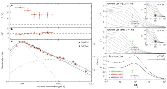
Figure 16.
(Left): Evolution of optical polarization (degree P (a), and position angle ((b); degrees east of north) and brightness ((c) in red (555–690 nm) light using RINGO2 and RATCam, in GRB 120308A (from [277]). (Right): 3 upper limits on the linear polarization of the radio flare emission from three different GRBs overlaid on the theoretical polarization light curves for a toroidal magnetic field in the GRB ejecta (from [111]). The top two panels are for a uniform (top-hat) jet where the different lines, from top to bottom, are for , while is the spectral index (in the observed radio band) and . In the top panel, the Lorentz factor of the ejecta is assumed to remain equal to that of the freshly shocked fluid just behind the forward shock (“FS”), while in the middle panel it is assumed to follow the Blandford and McKee [279] self-similar solution. The bottom panel is for a ‘‘structured’’ jet, in which the energy per solid angle drops as outside some small core angle.
The radio flar emission, e.g., [148,150,180,265,266,267], typically peaks on a timescale of a day or so (∼10 s). By this time, the shocked GRB ejecta shell settles in the back of the Blandford and McKee [279] self-similar solution, and its (∼5–10) is smaller by a factor of up to ∼1.5–1.8 compared to the material just behind the forward shock that dominates the afterglow emission at the same observed time [111,256]. This corresponds to a visible region of angle ∼0.1–0.2 rad around our line of sight, which is significantly larger than during the optical flash. Moreover, it often includes the entire jet (for a simple top-hat jet model) as suggested by the fact that the radio flare peak time is often comparable to the jet break time in the afterglow lightcurve. Granot and Taylor [111] have used VLA data of radio flares from three GRBs (990123, 991216, and 020405) to constrain its polarization, finding only upper limits for both linear and circular polarization. Their best limits are for GRB 991216, for which they found upper limits on the linear and circular polarization of 7% and 9%, respectively. These limits provide interesting constraints on GRB models and in particular are hard to reconcile with a predominantly ordered toroidal magnetic field in the GRB outflow together with a ‘‘structured’’ jet, where the energy per solid angle drops as the inverse square of the angle from the jet axis (see right panel of Figure 16). The polarization of the radio flare may be affected by the location of the observed frequency relative to the synchrotron self-absorption break frequency (polarization is suppressed when , during the rising phase of the radio flare) or by Faraday depolarization on the way from the source to us (both are discussed in [111]) and may also be subject to plasma propagation effects within the source (as discussed below, at the end of this section).
Comparing the polarization of the optical flash and radio flare for the same GRB would enable us to study the magnetic field in the GRB ejecta over a wide range of angular scales, probing magnetic structures with a coherence length over this angular range, . Measuring the reverse-shock emission polarization at intermediate times and frequencies, such as at sub-mm with ALMA (e.g., [265,267]), would provide a better coverage of this wide range. A particularly interesting example is GRB 190114C, which was also detected at TeV energies [280]. ALMA measured its sub-mm ( GHz) total intensity and linear polarization at 2.2 – 5.2 h after the burst, when the emission was dominated by the reverse shock [267], detecting linear polarization at confidence, decreasing from to , while the position angle evolved from to . This was the first detection and measurement of the temporal evolution of polarized radio/millimeter emission in a GRB. Using the measured linear polarization, Laskar et al. [267] constrained the coherence scale of tangled magnetic fields in the ejecta to an angular size of rad, while the rotation of the polarization angle rules out the presence of large-scale, ordered axisymmetric magnetic fields and, in particular, a large-scale toroidal field, in the jet.
6.3. Afterglow Emission
Linear polarization at the level of a few percent has been detected in the optical or NIR afterglow of about a dozen GRBs [22,281,282,283,284,285,286,287,288,289,290,291]. Higher levels of polarization () have been measured mostly in the very early afterglow, likely being dominated by reverse-shock emission, as discussed above (see, however, [292]). The linear polarization of the afterglow emission was considered as a confirmation that it arises primarily from synchrotron radiation, as was already suggested by its spectral energy distribution.
A variety of models have been suggested for GRB afterglow polarization: emission from different patches of uniform but mutually uncorrelated magnetic field, either with microlensing [293] or without it [63], or emission from a random magnetic field within the plane of the afterglow shock together with scintillation in the radio [64] or with a jet viewed not along its symmetry axis [223,294,295], possibly with the addition of an ordered component that pre-exists in the external medium and which is compressed by the afterglow shock and/or a tangled magnetic field that is not purely in the plane of the shock and may even be predominantly in the direction of the shock normal [109,296] or due to clumps in the external medium or a similarly inhomogeneous outflow [109,230].
The most popular models for GRB afterglow polarization feature an axis-symmetric jet viewed not along its symmetry axis along with a tangled shock-produced magnetic field that is symmetric about the local shock normal [109,112,143,222,223,294,295,297,298,299]. In such models, the only preferred direction on the plane of the sky is that connecting the jet symmetry axis and our LOS, and therefore the net polarization of the unresolved image must lie either along this direction or transverse to it. Indeed, the tell-tale signature of such models for a uniform top-hat jet is a change in the polarization PA as vanishes and reappears rotated by , around the time of the jet break in the afterglow lightcurve [223,294]. On the other hand, for a structured jet viewed from outside of its narrow core, a constant is expected. Overall, in such models the linear polarization and its temporal evolution depend on: (i) the jet’s angular structure, (ii) the local structure of the shock-generated magnetic field about the shock normal, and (iii) our viewing angle from the jet symmetry axis. Therefore, afterglow linear polarization observations can teach us both about the jet’s angular structure and about the shock-produced magnetic field structure. However, there is a significant degeneracy between the two, which usually requires making large assumptions about one of them in order to significantly constrain the other.
The exceptional case of the short GRB 170817A, which was associated with the first gravitational wave detection of the binary neutron star merger, GW 170817, has allowed us to break this degeneracy. This event was observed from a large off-axis viewing angle, and its low-luminosity prompt gamma-ray emission and subsequent long-lived afterglow emission could be observed thanks to its relatively small distance ( Mpc). The combination of an extremely well-monitored afterglow from radio to X-rays e.g., [168,169,170], and the super-luminal motion of its radio flux centroid ( between 75 and 230 days after the burst [300]) has allowed a good determination of our viewing angle and of the jet’s angular structure (e.g., [159,160,171,172,173,174,175,176,177,178,301,302]). This has enabled making robust predictions for the linear polarization that depend on the shock-produced magnetic field structure [172]. Shortly thereafter a linear polarization upper limit, (99% confidence), was set in the radio ( GHz) at days [303]. Assuming emission from a two-dimensional surface identified with the afterglow shock front, this has led to a constraint of on the magnetic field anisotropy parameter, [172,303], which was introduced by [109], where and are the magnetic field compenents parallel and perpendicular to the shock normal direction , respectively, and corresponds to an isotropic field in 3D (for which the local and global polarizations vanish). A more detailed analysis [112] accounted for the emission from the whole 3D volume behind the afterglow shock, with the global angular jet structure implied by the GRB 170817A/GW 170817 observation and a local radial hydrodynamic profile set by the Blandford and McKee [279] self-similar solution. The magnetic field was modeled as an isotropic field in 3D that is stretched along by a factor , whose initial value describes the field that survives downstream on plasma scales , and it is evolved downstream according to the [279] solution assuming flux freezing (i.e., no further magnetic dissipation or amplification far downstream of the shock front). In a local coordinate system where , in the above definition of b we have and due to the B-field’s symmetry about , while here in the definition of , represents either or but not (while ). Gill and Granot [112] found that the shock-produced magnetic field has a finite, but initially sub-dominant, parallel component: (see Figure 17).
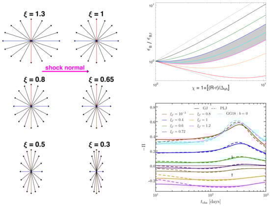
Figure 17.
Constraining the magnetic field structure in collisionless relativistic shocks from a radio afterglow linear polarization upper limit in GRB 170817/GW 170817 [112]. (Left): Schematic of post-shock magnetic field geometry for different values of the local anisotropy parameter , whose initial value just behind the shock is , for an external density profile , where is the Blandford and McKee [279] self-similar variable, r is the radial coordinate, and R and are the local radius and Lorentz factor of the afterglow shock front, respectively. (Top Right): The corresponding evolution of the magnetic field equipartition parameter, , with the distance behind the shock (as parameterized through ) for (from bottom to top). The two extreme values of are shown as dotted (straight) lines. The light-grey shaded region corresponds to the allowed range found in [112], . (Bottom Right): The linear polarization evolution, , obtained from a volume integration of the flow, shown for different values of . The two arrows mark the polarization upper limit, . Comparison was made between two jet structures–a Gaussian jet (GJ) and a power-law jet (PLJ). The result from [172], which assumed an infinitely thin shell geometry as well as locally isotropic synchrotron spectral emissivity, is also shown (labeled GG18) for the magnetic field anisotropy parameter .
Circular polarization at the level of has been reported in the optical afterglow of GRB 121024A [304] at days after the burst, when the linear polarization was , implying a relatively high circular-to-linear polarization ratio of . Nava et al. [305] performed a detailed analysis of the expected and in GRB afterglows, finding that while ad-hoc configurations may allow large local values, after transformations to the observer frame and integration over the whole visible region are performed, remains vanishingly small in any realistic optically thin synchrotron afterglow emission model and thus concluding that the origin of the observed in GRB 121024A cannot be intrinsic.
Plasma propagation effects due to the presence of cooler thermal electrons, which are not shock accelerated and represent a fraction of the total number, may be important if a significant ordered magnetic field component is present in the emitting region [306,307,308]. Such effects are most prominent in the early afterglow and around the self-absorption frequency and may therefore potentially affect the reverse shock emission (the “optical flash” or “radio flare”), as well as the forward shock emission in the radio up to a day or so [306,307,308]. These effects may include Faraday conversion of the linear polarization of the emitted radiation to circular polarization or Faraday depolarization of the emitted linear polarization. For typical GRB afterglow microphysical parameters, the latter effect may strongly suppress the linear polarization in the radio but preserve that in the optical. Therefore, simultaneous observations yielding statistically significant measurements of polarization in both optical and radio can be extremely useful to confirm the population of thermal electrons as well as the existence of an ordered B-field. In some GRBs, this effect may manifest in the sub-mm band where comparison between ALMA and VLA measurements can constrain the value of [308]. In fact, Urata et al. [309] argued that the unusually low afterglow polarization ( of GRB 171205A in the sub-mm band, as compared to the typical late-time optical polarization, may have been the result of Faraday depolarization. Since the true afterglow shock kinetic energy is given by [310], where E would be the true energy for , a constraint on would lead to better constraints on the burst energetics.
7. Outlook for 2030
The handful of successful -ray polarimeters has shown over the previous decade that although challenging, GRB polarization measurements are possible. With this new success, a range of new instruments with not only a higher sensitivity but also a wider energy range are foreseen to be launched over the coming decade. As mentioned earlier, however, simply increasing the number of measurements does not improve our understanding if different instruments provide incompatible results. Below we first discuss the promising advances in detector development for the coming decade. This is followed by a discussion on the need for improvements and standardization of the analysis.
7.1. Future Instruments
7.1.1. POLAR-2 and LEAP
In the Compton energy range of ∼10–1000 keV, four instruments are proposed. Both the LEAP [311] and SPHiNX [312] instruments have been proposed for launches in the coming decade, while the POLAR-2 project has already been accepted for launch in 2024 [313]. Additionally, the Daksha mission, a larger-scale full sky monitor follow-up mission based on the Astrosat CZTI is proposed to be launched in the coming decade as well [240]. Out of these four, the POLAR-2 and LEAP projects aim to make the next step in this field by producing instruments with an effective area an order of magnitude larger than the POLAR instrument. The SPHiNX project instead has an effective area similar to that of POLAR and will therefore have to make gains over currently existing measurements by aiming for a longer mission life time. For Daksha, the effective area is planned to be an order of magnitude larger than that of Astrosat CZTI. As the experiment will consist of two satellites, each observing half the sky, this increase in effective area is evenly distributed over the full sky. The design allows for a significant increase in the number of GRBs for which polarization measurements are possible, while also increasing the precision of each such measurement, although not by one full order of magnitude.
The POLAR-2 instrument is similar in design to POLAR with, apart from several minor design improvements, a focus on an improvement in three parts. The first is the size, which is four times larger than POLAR, resulting in a total geometrical area of approximately cm. Secondly, the scintillator readout technology is improved to decrease the low-energy threshold of the instrument from keV to keV, giving a total energy range of 20–800 keV for polarization measurements. Finally, POLAR-2 will be equipped with spectrometers making it independent of other instruments for spectral and location parameters of GRBs, which reduces the systematic error on many GRB measurements. The instrument was approved for launch in early 2024 towards the Chinese Space Station (CSS).
The LEAP instrument is similar to POLAR-2 both in size and in the detection mechanism that uses plastic scintillators. Contrary to POLAR-2, the LEAP instrument will also use high Z scintillators, which increase the absorption cross section. Therefore, the instrument will have a larger sensitivity to polarization and a better spectral response but a reduction in its effective area and field of view. Whereas the total effective area for LEAP that is useful for spectrometry is ∼ at , for polarization it is around ∼ [314]. For POLAR-2, the effective area of the polarimeter usable for spectrometry is ∼, and therefore significantly smaller than LEAP. For polarization, however, it is ∼ and therefore larger than LEAP. The reduction in effective area of the polarimeter for spectrometry in POLAR-2 is compensated by separate spectrometers, which will increase this by at least .
The two instruments therefore have different strengths. With a proposed launch in 2025 for LEAP towards the International Space Station (ISS), the combination of both of these instruments in orbit would allow for detailed polarization measurements of the majority of GRBs with fluences (as measured in the 10–1000 keV energy range) above .
7.1.2. Low-Energy Polarimeters
Apart from adding significant sensitivity in the energy range of ∼10–1000 keV, missions are also proposed to perform the first GRB polarization measurements at keV energies.
As previously mentioned, the first polarization measurements at these energies, albeit of point sources, were recently performed by the small scale PolarLite mission [195]. The IXPE mission [197], which uses a similar measurement technology as PolarLite, is planned to be launched in 2021. However, as it is optimized for point sources, it has a narrow FoV. This in combination with a long slewing time makes it unlikely to measure any GRBs. The larger-scale eXTP mission, however, will still be optimized for point sources but is designed to also observe targets of opportunity such as GRBs using a shorter slewing time. As such, eXTP will be capable of measuring the polarization of the afterglow of GRBs in the 2–10 keV energy range as well as any potential X-ray flares occurring in the afterglow [198]. eXTP is a joint Chinese–European mission and is currently foreseen to be launched in 2028.
The above-mentioned instruments are optimized for point sources and therefore have a small field of view to optimize the signal to noise. In order to measure the polarization of the prompt emission from GRBs, which appears at random positions in the sky, a relatively large field of view is required. A mission under consideration with this capability at keV energies is the Low-energy Polarimetry Detector (LPD) under development at the GuangXi University (Private communication with Prof. Hongbang Liu). The instrument is foreseen to have a sensitivity to polarization in the energy range of 2–30 keV and a maximum effective area of ∼ around 10 keV by using a similar technology as that used by Polarlight with an optimization of the gas for higher energies. The instrument is under consideration to be placed alongside POLAR-2 on the CSS, allowing to perform combined measurements of the prompt emission from 2 keV to 800 keV.
7.1.3. High-Energy Polarimeters
In the MeV energy range, one possible mission to be launched in the coming decade is AMEGO [315]. The AMEGO mission makes use of many layers of silicon placed on top of a calorimeter. This makes it ideal to perform polarization measurements using Compton scattering in the ∼ keV to MeV energy range. AMEGO will yield polarization measurements for the brightest of GRBs that it will observe.
A second instrument under development is a satellite version of the COSI balloon mission [316]. This instrument will make use of germanium strip detectors capable of measuring the three-dimensional interaction position of incoming photons. The energy range is similar to that of AMEGO ( keV to MeV). Thanks to its large field of view, it will observe around ∼40 GRBs per year with a fluence exceeding for which it can perform measurements with an MDP of around .
A highly promising instrument concept for polarimetry at MeV energies is the Advanced Particle-astrophysics Telescope [317]. The instrument is designed to maximize the effective area for photons in the MeV to TeV energies without using passive materials for photon conversion. The detector aims to use high Z scintillator crystals for the conversion in combination with scintillating fibres. This allows for a large-scale detector with precise measurements of both electron positron pairs and Compton-scattered photons. The current mission concept would be an order of magnitude more sensitive as a gamma-ray detector than Fermi-LAT and would be capable of performing polarization measurements at MeV energies for GRBs as weak as 170817A, for which an MDP of ∼40% was simulated. The project is in its early stages, and currently a path finder mission is planned for a balloon flight.
Apart from these two instruments the earlier-mentioned HARPO detector [200] will be capable of performing polarization measurements in the MeV energy range using pair production in a gas TPC. Unlike AMEGO and COSI, which are both under consideration for a launch in the coming decade, the HARPO instrument, of which a prototype has been successfully calibrated on ground [201], is currently not under consideration for a launch.
7.2. Performance Predictions
Generally, the coming decade looks promising. In the ∼10–1000 keV energy range a number of new detailed measurements are foreseen, which should be capable of resolving the current differences in PD reported by different groups. This is illustrated in Figure 18, which shows the yearly number of measurements capable of excluding a non-polarized flux as a function of the true polarization degree of GRBs for three different instruments, GAP, POLAR, and POLAR-2. For this figure, the instrument response of POLAR, as used in the POLAR analysis, was used as well as that for POLAR-2 in combination with the Fermi-GBM GRB catalog. For GAP, for which the response is not available, the numbers were produced by scaling the POLAR numbers based on the performance of GAP and POLAR for respectively detected GRBs, again in combination with the Fermi-GBM GRB catalog. It should be noted that for GAP, for which the detailed response is not known, a fixed was used, which, given its design, should be close to the truth.
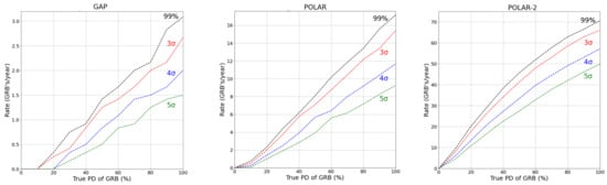
Figure 18.
The rate of measurements capable of excluding a non-polarized flux, for different confidence levels, as a function of the true polarization degree (PD) of GRBs for three different instruments, GAP, POLAR, and POLAR-2. Although exact numbers are not available it can be assumed that LEAP will be capable of similar rates as POLAR-2, albeit slightly lower.
It can be seen that with GAP excluding a non-polarized flux was possible for a handful of GRBs per year only in cases where the true PD of the emission is relatively high. For POLAR, the situation improves and, as was the case, with less than a year of data it was able to claim exclusion of polarization levels above ≈50%. It could not, however, effectively probe polarization levels below with a high confidence. With POLAR-2, this region will be probed within a few months, while with 1 year of data it will be capable of determining whether GRB emission is polarized to levels as low as . To illustrate the type of GRBs that can be probed with the different instruments, Figure 19 shows the mean MDP for the three different instruments as a function of the GRB fluence for both short (1 s observed duration) and long (100 s observed duration) GRBs. As an illustration, the fluence of the short and very weak GRB 170817A as well as the long and very bright GRB 190114C are added. It should be noted that the energy ranges used for the different instruments differs, and the energy range of 50–300 keV was used for GAP, 50–500 keV for POLAR and 20–500 keV for POLAR-2. Although no detailed response is available, the performance of LEAP is foreseen to be similar to that of POLAR-2 with a typical effective area ∼30% smaller than that of POLAR-2. A launch of LEAP would therefore further improve the situation, not only regarding the statistics but more importantly regarding the systematics. As for Daksha, not enough details on the instrument are available to make any clear predictions, while the SPHiNX performance would be similar to that of POLAR.
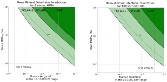
Figure 19.
The mean minimal detectable polarization for confidence level (MDP averaged over PA) as a function of the fluence in the 10–1000 keV energy band for GAP, POLAR, and POLAR-2 for both short ( s observed duration) and long ( s observed duration) GRBs. Short GRBs with a fluence above occur at a rate of approximately 10 per year on the full sky, whereas, for long GRBs, the rate is about 200 per year. For POLAR-2, the MDP for confidence is added as well, using a dotted line. The fluences of two well-known GRBs, the weak and short 170817A and the long and bright 190114C, were added as an illustration.
It is evident that the next generation of polarimeters will be capable of almost probing GRBs with fluences as weak as GRB 170817A, a GRB which was hard to even detect with both Fermi-GBM and INTEGRAL-SPI but was important due to its association with a gravitational wave signal [12]. Additionally, for very bright GRBs such as 190114C, which was observed at TeV energies [280,318], highly detailed polarization measurements will become possible, indicating that fine time or energy binning will become an available tool to study such GRBs. It should again be stressed that the mean MDP is simply a figure of merit and that the estimates given here are not exact, as the details will depend not only on the fluence and length of the GRBs but also on its energy spectrum, incoming angle, and position of the polarimeter along its orbit. Additionally, systematic errors, which can be significant, are not taken into account in an MDP calculation. The predictions should therefore be taken only to give an indication of the advancement in the field as well as the possibilities during the coming decade.
Apart from an improvement in the Compton scattering regime, the first polarization measurements of the prompt emission at MeV energies can be expected towards the end of this decade. There still remains an additional need for energy-dependent polarization measurements. Whereas the eXTP instrument can probe the polarization at keV energies, it is unlikely to detect the prompt emission due to its narrow field of view. An instrument such as the LPD would, especially when placed closed to POLAR-2, allow to provide an energy range of 2–800 keV for many GRBs per year. This would allow to study a potential change in PD in the 10–50 keV energy range, as proposed in some photospheric emission models [232]. In addition, if either COSI or AMEGO will be launched, detailed energy-resolved studies will become possible for bright GRBs in the 2 keV to 5 MeV energy range, thereby fully probing the prompt emission over several orders of magnitude in energy.
7.3. Improvements in Analysis
From the measurement results published to date, it can be seen that increasing the number of measurements alone is likely not enough to provide clear conclusions on the polarization of GRB prompt emission. The clearest example of this is the discrepancy between the results of POLAR and Astrosat CZTI. Out of the 11 GRBs analysed by the Astrosat CZTI collaboration in [188], the six GRBs for which statistically significant measurements (based on the calculation of a Bayes factor required to be above tow) are possible, the polarization levels for all exceeds . For 12 out of the 14 GRB, measurements presented by POLAR the PD were found to be below with the two remaining having a low significance. Although the number of measurements is low, the difference in the results is striking. In order to advance the field, it is prudent to first understand the cause of these differences in these results as well as other earlier published results.
7.3.1. Need for Public Analysis Tools and Data
Polarization analysis is complex, and mistakes can easily lead to high levels of PD being measured. As the field is not yet mature and collaborations are small, every analysis has so far almost exclusively been performed using a tool developed for that specific data. This constant reinvention of the wheel not only allows for mistakes but more importantly results in instrument-specific analysis tools. Such tools are incapable of being applied to other data, and their performance is difficult to verify by a referee or other interested scientists. If, additionally, the code and the data are not public, as is often the case, and publications lack details on the analysis, then it remains nearly impossible to investigate discrepancies with other results.
What is therefore required, arguably more so than more measurements, is a standardized analysis method, which can be adapted to each polarimeter with a public code. Such tools, similar to those widely used in spectrometry such as Xspec [319] and 3 ML, would not only allow to understand any potential discrepancies but would also remove the need to reinvent the method by each new collaboration. Furthermore, if additional instrument data and responses exist publicly, it would remove the requirement to have an in-depth understanding of the instrument for being able to perform analysis. This would allow, similar to what happens in spectrometry, for experts in the field of data analysis and statistics to perform the analysis instead of only instrument experts as is now often the case, allowing for more detailed and innovative analyses to be performed.
A first step towards this was produced as part of the 3ML framework [320] for the analysis of the POLAR data. The developed tools aim to provide a framework in which the instrument response and the measurement data are combined to perform the polarization analysis in a transparent way that is usable by anyone. Both for the instrument response and the data format, a standardized format is proposed similar to that used in spectrometry, and the tool can therefore easily be adapted for other polarimeters. The tool has been used first to analyze GRB 170114A [104] in detail using POLAR data, and subsequently to produce the full GRB catalog published by POLAR [187]. The POLAR data used for this analysis is furthermore public https://www.astro.unige.ch/polar/grb-light-curves (accessed on 25 August 2014), allowing further analysis by anyone interested as well as to perform rigorous tests of the validity of the different POLAR results. The public data alone could, for example, already be used by the Astrosat CZTI collaboration using the tools used for the results in [188] to find if their tools provide consistent results are those published in [187]. Although not perfect, such a study would arguably progress the field further than the analysis of additional Astrosat CZTI or POLAR data by the collaborations themselves.
7.3.2. Multi-Instrument Analysis
Thanks to the properties of the 3ML framework, data from different instruments can be combined. So far, this feature was used only to combine the POLAR data with that from Fermi-GBM and Swift-BAT. This allowed to improve the spectral fits, as the error on the spectrum adds to the systematic error on the polarization measurement, which in turn led to more precise polarization measurements. The 3ML framework additionally allows to fit physical models directly to the data, rather than fitting the data with empirical models and subsequently comparing the results with a parameterized outcome of a theoretical prediction. Although easier, the latter method has, especially in the field of gamma-ray spectrometry, been found to result in over-interpretation of data analysis results and to inconsistent conclusions (see discussion in Section 2.3.1). The fitting of physical models directly to data is especially desirable in the field of polarimetry as it allows to fit these models, potentially unbinned in time and energy, directly both to spectral and polarization data at the same time.
Apart from combining spectral and polarization data in the analysis, in theory, the same can be done using data from two polarimeters in case two different polarimeters observed the same GRB. In fact, several GRBs were observed by both Astrosat and POLAR [187,321]. It would therefore be highly desirable to perform combined analysis of the Astrosat and POLAR data for such GRBs as it would, firstly, allow to study the cause of the likely discrepancy between the results from both instruments. Secondly, it can allow for more detailed measurements of the polarization of these GRBs.
With upcoming instruments sensitive in different energy ranges, such analysis tools will in the future allow to fit physical models to both spectral and polarization data over a broad range in energy by, for example, combining the data of the LPD, LEAP, POLAR-2, and AMEGO or COSI. Whereas with the current level of polarimetry analysis tools, the data has to be studied separately, leaving the full potential of the data unexploited.
As the polarization tool in the 3ML framework discussed here is new and has not been used for the polarization analysis of other instruments, it is to be seen if it will be used by the wider community. However, with the potential of two large-scale polarimeters in LEAP and POLAR-2 launching in the coming years, as well as polarimeters sensitive at keV and at MeV energies, there is a clear need for a collaborative effort between the groups to either further develop this tool or construct a completely new one.
7.4. Improvements in Theoretical Modeling of Prompt GRB Polarization
Pulse-integrated polarization from semi-analytic models of axisymmetric flows with different prompt GRB radiation mechanisms and B-field configurations have been presented in many works [20,24,108,109,110,111,134]. The same setup was used to make predictions for the time-dependent polarization for synchrotron emission in some works [84,322,323]. On the other hand, only a few works have attacked the problem using MC simulations [56,57,58] or radial integration of the transfer equations for the Stokes parameters [55]. Many of these have focused only on photospheric emission.
As the next decade may see the launch of more sensitive instruments to measure GRB polarization with high fidelity, it calls for time- and energy-dependent polarization predictions (, ) for more realistic outflow models, which would also predict the time-dependent flux density, .
One of the weaknesses of current theoretical models is the assumption of an axisymmetric flow, which is usually made for simplicity and convenience. This restricts the change in PA to only , whereas some observations do show, although not so convincingly yet, hints of gradual PA swings. To obtain a change in the PA other than or to get a gradually changing PA, the condition for axisymmetry must be broken, e.g., the magnetic field configuration/orientation and/or the emissivity can change as a function of .
One possibility is that the different pulses that contribute to the emission arise in “mini-jets” within the outflow e.g., [32,85,324,325,326,327]. In this case, the different directions of the mini-jets or bright patches w.r.t. the LOS (e.g., [109,230]) would cause the PA to also be different between the pulses even for a field that is locally symmetric w.r.t the local radial direction (e.g., or ) as well as for fields that are axisymmetric w.r.t to the center of each mini-jet (e.g., a local for each mini-jet). Finally, broadly similar results would follow from an ordered field within each mini-jet (), which are incoherent between different mini-jets. Time-resolved measurement in such a case would naturally yield a time-varying PA.
Alternatively, as shown by Granot and Königl [109] for GRB afterglow polarization, a combination of an ordered field component (e.g., ) and a random field, like , can give rise to a time-varying PA between different pulses (with a different ratio of the two field components) that cab, e.g., arise from internal shocks. The ordered field component here would be that advected from the central enginem and the random field component can be argued to be shock-generated. Notice that the ordered field component should not be axisymmetric in order for the position angle to smoothly vary.
Realistic theoretical predictions can be obtained by coupling radiation transfer modeling with MHD numerical simulations of relativistic jets after they break out of the confining medium. A step towards this direction was taken by Parsotan et al. [58] who used the MHD code FLASH to first obtain the jet’s angular structure by injecting variable jets into stellar density profiles of Wolf–Rayet stars at core-collapse. They then used an MC code to carry out the radiation transfer of the Stokes parameters and obtain the time-resolved polarization for the photospheric emission (see Figure 10). In another recent work, Ito et al. [328] carried out global neutrino-hydrodynamic simulations of a relativistic jet launched in a binary NS merger scenario. The photospheric emission and polarization from the short GRB was then calculated using a relativistic MC code. While these works focused only on photospheric emission, polarization modeling for other radiation mechanisms performed in the same vein is lacking and can prove to be very fruitful.
MC radiation transfer and MHD numerical simulations of relativistic jets can be computationally expensive. They are nevertheless a useful tool that can be used to calibrate semi-analytic models by delineating the relevant parameter space expected in GRB jets. Ultimately, when high quality observations are made in this decade, fast and computationally inexpensive theoretical models will be required to carry out time-resolved spectro-polarimetric fits in a reasonable amount of time. This further stresses the need for a library of models, akin to Xspec [319] that is used routinely for spectral fitting or boxfit [329] for GRB afterglow lightcurve modeling, which can be conveniently used by observers. Combining the library of models with the 3ML framework for spectro-polarimetric data analysis will become a very powerful tool for GRB science.
In order to test the different model predictions, e.g., from different radiation mechanisms, on an equal footing, a single underlying theoretical framework should be devised for the jet structure and dynamics, which allows the same freedom in the different model parameters. Such an approach can help to isolate the dominant prompt GRB radiation mechanism when compared with observations.
To conclude, the next decade appears very promising for answering many fundamental questions in GRB physics. With the launch of several dedicated instruments capable of performing high-fidelity -ray and X-ray spectro-polarimetry, a larger sample of statistically significant prompt GRB polarization measurements will be obtained. Improvements in polarization data analysis using a single underlying framework that allows simultaneous fitting of both spectrum and polarization from different instruments will yield unbiased and high-quality results. More realistic theoretical models of both time- and energy-dependent polarization based on advanced numerical simulations will allow to better understand the true nature of GRB jets.
Author Contributions
Writing—original draft preparation—review and editing, R.G., M.K. and J.G. All authors have read and agreed to the published version of the manuscript.
Funding
This research was funded in part by the ISF-NSFC joint research program under grant no. 3296/19 (R.G. and J.G.) and the Swiss National Science Foundation (M.K.).
Institutional Review Board Statement
Not applicable.
Informed Consent Statement
Not applicable.
Data Availability Statement
No new data were created or analyzed in this study. Data sharing is not applicable to this article.
Acknowledgments
We thank Stefano Covino and Mark McConnell for a thorough read of an earlier version of the manuscript and for their comments and feedback.
Conflicts of Interest
The authors declare no conflict of interest.
References
- Kouveliotou, C.; Meegan, C.A.; Fishman, G.J.; Bhat, N.P.; Briggs, M.S.; Koshut, T.M.; Paciesas, W.S.; Pendleton, G.N. Identification of Two Classes of Gamma-ray Bursts. Astrophys. J. 1993, 413, L101. [Google Scholar] [CrossRef]
- Fruchter, A.S.; Levan, A.J.; Strolger, L.; Vreeswijk, P.M.; Thorsett, S.E.; Bersier, D.; Burud, I.; Castro Cerón, J.M.; Castro-Tirado, A.J.; Conselice, C.; et al. Long γ-ray bursts and core-collapse supernovae have different environments. Nature 2006, 441, 463–468. [Google Scholar] [CrossRef]
- Galama, T.J.; Vreeswijk, P.M.; van Paradijs, J.; Kouveliotou, C.; Augusteijn, T.; Böhnhardt, H.; Brewer, J.P.; Doublier, V.; Gonzalez, J.F.; Leibundgut, B.; et al. An unusual supernova in the error box of the γ-ray burst of 25 April 1998. Nature 1998, 395, 670–672. [Google Scholar] [CrossRef]
- Hjorth, J.; Sollerman, J.; Møller, P.; Fynbo, J.P.U.; Woosley, S.E.; Kouveliotou, C.; Tanvir, N.R.; Greiner, J.; Andersen, M.I.; Castro-Tirado, A.J.; et al. A very energetic supernova associated with the γ-ray burst of 29 March 2003. Nature 2003, 423, 847–850. [Google Scholar] [CrossRef] [PubMed]
- Stanek, K.Z.; Matheson, T.; Garnavich, P.M.; Martini, P.; Berlind, P.; Caldwell, N.; Challis, P.; Brown, W.R.; Schild, R.; Krisciunas, K.; et al. Spectroscopic Discovery of the Supernova 2003dh Associated with GRB 030329. Astrophys. J. 2003, 591, L17–L20. [Google Scholar] [CrossRef]
- Gehrels, N.; Sarazin, C.L.; O’Brien, P.T.; Zhang, B.; Barbier, L.; Barthelmy, S.D.; Blustin, A.; Burrows, D.N.; Cannizzo, J.; Cummings, J.R.; et al. A short γ-ray burst apparently associated with an elliptical galaxy at redshift z = 0.225. Nature 2005, 437, 851–854. [Google Scholar] [CrossRef]
- Barthelmy, S.D.; Chincarini, G.; Burrows, D.N.; Gehrels, N.; Covino, S.; Moretti, A.; Romano, P.; O’Brien, P.T.; Sarazin, C.L.; Kouveliotou, C.; et al. An origin for short γ-ray bursts unassociated with current star formation. Nature 2005, 438, 994–996. [Google Scholar] [CrossRef]
- Woosley, S.E. Gamma-ray Bursts from Stellar Mass Accretion Disks around Black Holes. Astrophys. J. 1993, 405, 273. [Google Scholar] [CrossRef]
- Eichler, D.; Livio, M.; Piran, T.; Schramm, D.N. Nucleosynthesis, neutrino bursts and Gamma-rays from coalescing neutron stars. Nature 1989, 340, 126–128. [Google Scholar] [CrossRef]
- Narayan, R.; Paczynski, B.; Piran, T. Gamma-ray bursts as the death throes of massive binary stars. Astrophys. J. 1992, 395, L83–L86. [Google Scholar] [CrossRef]
- Abbott, B.P.; Abbott, R.; Abbott, T.D.; Acernese, F.; Ackley, K.; Adams, C.; Adams, T.; Addesso, P.; Adhikari, R.X.; Adya, V.B.; et al. GW170817: Observation of Gravitational Waves from a Binary Neutron Star Inspiral. Phys. Rev. Lett. 2017, 119, 161101. [Google Scholar] [CrossRef] [PubMed]
- Abbott, B.P.; Abbott, R.; Abbott, T.D.; Acernese, F.; Ackley, K.; Adams, C.; Adams, T.; Addesso, P.; Adhikari, R.X.; Adya, V.B.; et al. Gravitational Waves and Gamma-rays from a Binary Neutron Star Merger: GW170817 and GRB 170817A. Astrophys. J. 2017, 848, L13. [Google Scholar] [CrossRef]
- Band, D.; Matteson, J.; Ford, L.; Schaefer, B.; Palmer, D.; Teegarden, B.; Cline, T.; Briggs, M.; Paciesas, W.; Pendleton, G.; et al. BATSE Observations of Gamma-ray Burst Spectra. I. Spectral Diversity. Astrophys. J. 1993, 413, 281. [Google Scholar] [CrossRef]
- Preece, R.D.; Briggs, M.S.; Mallozzi, R.S.; Pendleton, G.N.; Paciesas, W.S.; Band, D.L. The BATSE Gamma-ray Burst Spectral Catalog. I. High Time Resolution Spectroscopy of Bright Bursts Using High Energy Resolution Data. Astrophys. J. Suppl. Ser. 2000, 126, 19–36. [Google Scholar] [CrossRef]
- Kaneko, Y.; Preece, R.D.; Briggs, M.S.; Paciesas, W.S.; Meegan, C.A.; Band, D.L. The Complete Spectral Catalog of Bright BATSE Gamma-ray Bursts. Astrophys. J. Suppl. Ser. 2006, 166, 298–340. [Google Scholar] [CrossRef]
- Coburn, W.; Boggs, S.E. Polarization of the prompt γ-ray emission from the γ-ray burst of 6 December 2002. Nature 2003, 423, 415–417. [Google Scholar] [CrossRef]
- Rutledge, R.E.; Fox, D.B. Re-analysis of polarization in the gamma-ray flux of GRB 021206. Mon. Not. R. Astron. Soc. 2004, 350, 1288–1300. [Google Scholar] [CrossRef]
- Wigger, C.; Hajdas, W.; Arzner, K.; Gudel, M.; Zehnder, A. Gamma-ray burst polarization: Limits from rhessi measurements. Astrophys. J. 2004, 613, 1088–1100. [Google Scholar] [CrossRef]
- Lazzati, D. Polarization in the prompt emission of gamma-ray bursts and their afterglows. New J. Phys. 2006, 8, 131. [Google Scholar] [CrossRef]
- Toma, K.; Sakamoto, T.; Zhang, B.; Hill, J.E.; McConnell, M.L.; Bloser, P.F.; Yamazaki, R.; Ioka, K.; Nakamura, T. Statistical Properties of Gamma-ray Burst Polarization. Astrophys. J. 2009, 698, 1042–1053. [Google Scholar] [CrossRef]
- Toma, K. Polarization of GRB Prompt Emission. arXiv 2013, arXiv:1308.5733. [Google Scholar]
- Covino, S.; Gotz, D. Polarization of prompt and afterglow emission of Gamma-Ray Bursts. Astron. Astrophys. Trans. 2016, 29, 205–244. [Google Scholar]
- McConnell, M.L. High energy polarimetry of prompt GRB emission. New Astron. Rev. 2017, 76, 1–21. [Google Scholar] [CrossRef]
- Gill, R.; Granot, J.; Kumar, P. Linear polarization in gamma-ray burst prompt emission. Mon. Not. R. Astron. Soc. 2020, 491, 3343–3373. [Google Scholar] [CrossRef]
- Piran, T. The physics of Gamma-ray bursts. Rev. Mod. Phys. 2004, 76, 1143–1210. [Google Scholar] [CrossRef]
- Zhang, B.; Mészáros, P. Gamma-Ray Bursts: Progress, problems & prospects. Int. J. Mod. Phys. A 2004, 19, 2385–2472. [Google Scholar] [CrossRef]
- Mészáros, P. Gamma-ray bursts. Rep. Prog. Phys. 2006, 69, 2259–2321. [Google Scholar] [CrossRef]
- Granot, J.; Ramirez-Ruiz, E. Jets and gamma-ray burst unification schemes. Gamma-Ray Bursts 2012, 51, 215. [Google Scholar]
- Kumar, P.; Zhang, B. The physics of gamma-ray bursts & relativistic jets. Phys. Rep. 2015, 561, 1–109. [Google Scholar]
- Rees, M.J.; Meszaros, P. Unsteady Outflow Models for Cosmological Gamma-Ray Bursts. Astrophys. J. 1994, 430, L93. [Google Scholar] [CrossRef]
- Thompson, C. A Model of Gamma-Ray Bursts. Mon. Not. R. Astron. Soc. 1994, 270, 480. [Google Scholar] [CrossRef]
- Lyutikov, M.; Blandford, R. Gamma Ray Bursts as Electromagnetic Outflows. arXiv 2003, arXiv:astro-ph/0312347. [Google Scholar]
- Goodman, J. Are gamma-ray bursts optically thick? Astrophys. J. 1986, 308, L47. [Google Scholar] [CrossRef]
- Paczynski, B. Gamma-ray bursters at cosmological distances. Astrophys. J. 1986, 308, L43–L46. [Google Scholar] [CrossRef]
- Li, Z.Y.; Chiueh, T.; Begelman, M.C. Electromagnetically Driven Relativistic Jets: A Class of Self-similar Solutions. Astrophys. J. 1992, 394, 459. [Google Scholar] [CrossRef]
- Vlahakis, N.; Königl, A. Relativistic Magnetohydrodynamics with Application to Gamma-Ray Burst Outflows. I. Theory and Semianalytic Trans-Alfvénic Solutions. Astrophys. J. 2003, 596, 1080–1103. [Google Scholar] [CrossRef]
- Beskin, V.S.; Nokhrina, E.E. The effective acceleration of plasma outflow in the paraboloidal magnetic field. Mon. Not. R. Astron. Soc. 2006, 367, 375–386. [Google Scholar] [CrossRef]
- Lyubarsky, Y.E. Transformation of the Poynting flux into kinetic energy in relativistic jets. Mon. Not. R. Astron. Soc. 2010, 402, 353–361. [Google Scholar] [CrossRef]
- Komissarov, S.S.; Vlahakis, N.; Königl, A.; Barkov, M.V. Magnetic acceleration of ultrarelativistic jets in gamma-ray burst sources. Mon. Not. R. Astron. Soc. 2009, 394, 1182–1212. [Google Scholar] [CrossRef]
- Goldreich, P.; Julian, W.H. Stellar Winds. Astrophys. J. 1970, 160, 971. [Google Scholar] [CrossRef]
- Lyubarsky, Y. Asymptotic Structure of Poynting-Dominated Jets. Astrophys. J. 2009, 698, 1570–1589. [Google Scholar] [CrossRef]
- Ruderman, M. Theories of gamma-ray bursts. In Seventh Texas Symposium on Relativistic Astrophysics; New York Academy of Sciences: New York, NY, USA, 1975; Volume 262, pp. 164–180. [Google Scholar] [CrossRef]
- Tchekhovskoy, A.; Narayan, R.; McKinney, J.C. Magnetohydrodynamic simulations of Gamma-ray burst jets: Beyond the progenitor star. New Astron. 2010, 15, 749–754. [Google Scholar] [CrossRef]
- Komissarov, S.S.; Vlahakis, N.; Königl, A. Rarefaction acceleration of ultrarelativistic magnetized jets in gamma-ray burst sources. Mon. Not. R. Astron. Soc. 2010, 407, 17–28. [Google Scholar] [CrossRef]
- Granot, J.; Komissarov, S.S.; Spitkovsky, A. Impulsive acceleration of strongly magnetized relativistic flows. Mon. Not. R. Astron. Soc. 2011, 411, 1323–1353. [Google Scholar] [CrossRef]
- Granot, J. The effects of sub-shells in highly magnetized relativistic flows. Mon. Not. R. Astron. Soc. 2012, 421, 2467–2477. [Google Scholar] [CrossRef][Green Version]
- Lyubarsky, Y.; Kirk, J.G. Reconnection in a Striped Pulsar Wind. Astrophys. J. 2001, 547, 437–448. [Google Scholar] [CrossRef]
- Spruit, H.C.; Daigne, F.; Drenkhahn, G. Large scale magnetic fields and their dissipation in GRB fireballs. Astron. Astrophys. 2001, 369, 694–705. [Google Scholar] [CrossRef]
- Drenkhahn, G. Acceleration of GRB outflows by Poynting flux dissipation. Astron. Astrophys. 2002, 387, 714–724. [Google Scholar] [CrossRef]
- Drenkhahn, G.; Spruit, H.C. Efficient acceleration and radiation in Poynting flux powered GRB outflows. Astron. Astrophys. 2002, 391, 1141–1153. [Google Scholar] [CrossRef]
- Bégué, D.; Pe’er, A.; Lyubarsky, Y. Radiative striped wind model for gamma-ray bursts. Mon. Not. R. Astron. Soc. 2017, 467, 2594–2611. [Google Scholar] [CrossRef]
- Lyutikov, M. The electromagnetic model of gamma-ray bursts. New J. Phys. 2006, 8, 119. [Google Scholar] [CrossRef]
- Pe’er, A. Temporal Evolution of Thermal Emission from Relativistically Expanding Plasma. Astrophys. J. 2008, 682, 463–473. [Google Scholar] [CrossRef]
- Beloborodov, A.M. Collisional mechanism for gamma-ray burst emission. Mon. Not. R. Astron. Soc. 2010, 407, 1033–1047. [Google Scholar] [CrossRef]
- Beloborodov, A.M. Radiative Transfer in Ultrarelativistic Outflows. Astrophys. J. 2011, 737, 68. [Google Scholar] [CrossRef]
- Ito, H.; Nagataki, S.; Matsumoto, J.; Lee, S.H.; Tolstov, A.; Mao, J.; Dainotti, M.; Mizuta, A. Spectral and Polarization Properties of Photospheric Emission from Stratified Jets. Astrophys. J. 2014, 789, 159. [Google Scholar] [CrossRef]
- Lundman, C.; Pe’er, A.; Ryde, F. Polarization properties of photospheric emission from relativistic, collimated outflows. Mon. Not. R. Astron. Soc. 2014, 440, 3292–3308. [Google Scholar] [CrossRef]
- Parsotan, T.; López-Cámara, D.; Lazzati, D. Photospheric Polarization Signatures from Long Gamma-ray Burst Simulations. Astrophys. J. 2020, 896, 139. [Google Scholar] [CrossRef]
- Papathanassiou, H.; Meszaros, P. Spectra of Unsteady Wind Models of Gamma-ray Bursts. Astrophys. J. 1996, 471, L91. [Google Scholar] [CrossRef]
- Sari, R.; Piran, T. Variability in Gamma-ray Bursts: A Clue. Astrophys. J. 1997, 485, 270–273. [Google Scholar] [CrossRef]
- Daigne, F.; Mochkovitch, R. Gamma-ray bursts from internal shocks in a relativistic wind: Temporal and spectral properties. Mon. Not. R. Astron. Soc. 1998, 296, 275–286. [Google Scholar] [CrossRef]
- Weibel, E.S. Spontaneously Growing Transverse Waves in a Plasma Due to an Anisotropic Velocity Distribution. Phys. Rev. Lett. 1959, 2, 83–84. [Google Scholar] [CrossRef]
- Gruzinov, A.; Waxman, E. Gamma-ray Burst Afterglow: Polarization and Analytic Light Curves. Astrophys. J. 1999, 511, 852–861. [Google Scholar] [CrossRef]
- Medvedev, M.V.; Loeb, A. Generation of Magnetic Fields in the Relativistic Shock of Gamma-ray Burst Sources. Astrophys. J. 1999, 526, 697–706. [Google Scholar] [CrossRef]
- Bret, A. Weibel, Two-Stream, Filamentation, Oblique, Bell, Buneman… Which One Grows Faster? Astrophys. J. 2009, 699, 990–1003. [Google Scholar] [CrossRef]
- Keshet, U.; Katz, B.; Spitkovsky, A.; Waxman, E. Magnetic Field Evolution in Relativistic Unmagnetized Collisionless Shocks. Astrophys. J. 2009, 693, L127–L130. [Google Scholar] [CrossRef]
- Sironi, L.; Goodman, J. Production of Magnetic Energy by Macroscopic Turbulence in GRB Afterglows. Astrophys. J. 2007, 671, 1858–1867. [Google Scholar] [CrossRef]
- Zhang, W.; MacFadyen, A.; Wang, P. Three-Dimensional Relativistic Magnetohydrodynamic Simulations of the Kelvin-Helmholtz Instability: Magnetic Field Amplification by a Turbulent Dynamo. Astrophys. J. 2009, 692, L40–L44. [Google Scholar] [CrossRef]
- Inoue, T.; Asano, K.; Ioka, K. Three-dimensional Simulations of Magnetohydrodynamic Turbulence Behind Relativistic Shock Waves and Their Implications for Gamma-ray Bursts. Astrophys. J. 2011, 734, 77. [Google Scholar] [CrossRef]
- Mizuno, Y.; Pohl, M.; Niemiec, J.; Zhang, B.; Nishikawa, K.I.; Hardee, P.E. Magnetic-field Amplification by Turbulence in a Relativistic Shock Propagating Through an Inhomogeneous Medium. Astrophys. J. 2011, 726, 62. [Google Scholar] [CrossRef]
- Mizuno, Y.; Pohl, M.; Niemiec, J.; Zhang, B.; Nishikawa, K.I.; Hardee, P.E. Magnetic field amplification and saturation in turbulence behind a relativistic shock. Mon. Not. R. Astron. Soc. 2014, 439, 3490–3503. [Google Scholar] [CrossRef]
- del Valle, M.V.; Lazarian, A.; Santos-Lima, R. Turbulence-induced magnetic fields in shock precursors. Mon. Not. R. Astron. Soc. 2016, 458, 1645–1659. [Google Scholar] [CrossRef]
- Romanova, M.M.; Lovelace, R.V.E. Magnetic field, reconnection and particle acceleration in extragalactic jets. Astron. Astrophys. 1992, 262, 26–36. [Google Scholar]
- Lyubarskij, Y.E. Energy release in strongly magnetized relativistic winds. Sov. Astron. Lett. 1992, 18, 356. [Google Scholar]
- Eichler, D. Magnetic Confinement of Jets. Astrophys. J. 1993, 419, 111. [Google Scholar] [CrossRef]
- Begelman, M.C. Instability of Toroidal Magnetic Field in Jets and Plerions. Astrophys. J. 1998, 493, 291–300. [Google Scholar] [CrossRef]
- Giannios, D.; Spruit, H.C. The role of kink instability in Poynting-flux dominated jets. Astron. Astrophys. 2006, 450, 887–898. [Google Scholar] [CrossRef]
- Levinson, A.; Begelman, M.C. Collimation and Confinement of Magnetic Jets by External Media. Astrophys. J. 2013, 764, 148. [Google Scholar] [CrossRef]
- McKinney, J.C.; Uzdensky, D.A. A reconnection switch to trigger Gamma-ray burst jet dissipation. Mon. Not. R. Astron. Soc. 2012, 419, 573–607. [Google Scholar] [CrossRef]
- Davis, S.W.; Stone, J.M.; Pessah, M.E. Sustained Magnetorotational Turbulence in Local Simulations of Stratified Disks with Zero Net Magnetic Flux. Astrophys. J. 2010, 713, 52–65. [Google Scholar] [CrossRef]
- O’Neill, S.M.; Reynolds, C.S.; Miller, M.C.; Sorathia, K.A. Low-frequency Oscillations in Global Simulations of Black Hole Accretion. Astrophys. J. 2011, 736, 107. [Google Scholar] [CrossRef]
- Giannios, D.; Uzdensky, D.A. GRB and blazar jets shining through their stripes. Mon. Not. R. Astron. Soc. 2019, 484, 1378–1389. [Google Scholar] [CrossRef]
- Tchekhovskoy, A.; McKinney, J.C.; Narayan, R. Simulations of ultrarelativistic magnetodynamic jets from Gamma-ray burst engines. Mon. Not. R. Astron. Soc. 2008, 388, 551–572. [Google Scholar] [CrossRef]
- Gill, R.; Granot, J. Temporal Evolution of Prompt GRB Polarization. arXiv 2021, arXiv:2101.06777. [Google Scholar]
- Zhang, B.; Yan, H. The Internal-collision-induced Magnetic Reconnection and Turbulence (ICMART) Model of Gamma-ray Bursts. Astrophys. J. 2011, 726, 90. [Google Scholar] [CrossRef]
- Deng, W.; Zhang, H.; Zhang, B.; Li, H. Collision-induced Magnetic Reconnection and a Unified Interpretation of Polarization Properties of GRBs and Blazars. Astrophys. J. 2016, 821, L12. [Google Scholar] [CrossRef]
- Sari, R.; Piran, T.; Narayan, R. Spectra and Light Curves of Gamma-ray Burst Afterglows. Astrophys. J. 1998, 497, L17–L20. [Google Scholar] [CrossRef]
- Granot, J.; Sari, R. The Shape of Spectral Breaks in Gamma-ray Burst Afterglows. Astrophys. J. 2002, 568, 820–829. [Google Scholar] [CrossRef]
- Crider, A.; Liang, E.P.; Smith, I.A.; Preece, R.D.; Briggs, M.S.; Pendleton, G.N.; Paciesas, W.S.; Band, D.L.; Matteson, J.L. Evolution of the Low-Energy Photon Spectral in Gamma-ray Bursts. Astrophys. J. 1997, 479, L39–L42. [Google Scholar] [CrossRef]
- Preece, R.D.; Briggs, M.S.; Mallozzi, R.S.; Pendleton, G.N.; Paciesas, W.S.; Band, D.L. The Synchrotron Shock Model Confronts a “Line of Death” in the BATSE Gamma-ray Burst Data. Astrophys. J. 1998, 506, L23–L26. [Google Scholar] [CrossRef]
- Preece, R.D.; Briggs, M.S.; Giblin, T.W.; Mallozzi, R.S.; Pendleton, G.N.; Paciesas, W.S.; Band, D.L. On the Consistency of Gamma-ray Burst Spectral Indices with the Synchrotron Shock Model. Astrophys. J. 2002, 581, 1248–1255. [Google Scholar] [CrossRef]
- Ghirlanda, G.; Celotti, A.; Ghisellini, G. Extremely hard GRB spectra prune down the forest of emission models. Astron. Astrophys. 2003, 406, 879–892. [Google Scholar] [CrossRef]
- Lloyd, N.M.; Petrosian, V. Synchrotron Radiation as the Source of Gamma-ray Burst Spectra. Astrophys. J. 2000, 543, 722–732. [Google Scholar] [CrossRef]
- Medvedev, M.V. Theory of “Jitter” Radiation from Small-Scale Random Magnetic Fields and Prompt Emission from Gamma-ray Burst Shocks. Astrophys. J. 2000, 540, 704–714. [Google Scholar] [CrossRef][Green Version]
- Mészáros, P.; Rees, M.J. Steep Slopes and Preferred Breaks in Gamma-ray Burst Spectra: The Role of Photospheres and Comptonization. Astrophys. J. 2000, 530, 292–298. [Google Scholar] [CrossRef]
- Burgess, J.M.; Ryde, F.; Yu, H.F. Taking the band function too far: A tale of two α’s. Mon. Not. R. Astron. Soc. 2015, 451, 1511–1521. [Google Scholar] [CrossRef]
- Poolakkil, S.; Preece, R.; Fletcher, C.; Goldstein, A.; Bhat, P.N.; Bissaldi, E.; Briggs, M.S.; Burns, E.; Cleveland, W.H.; Giles, M.M.; et al. The Fermi-GBM Gamma-ray Burst Spectral Catalog: 10 yr of Data. Astrophys. J. 2021, 913, 60. [Google Scholar] [CrossRef]
- Gruber, D.; Goldstein, A.; Weller von Ahlefeld, V.; Narayana Bhat, P.; Bissaldi, E.; Briggs, M.S.; Byrne, D.; Cleveland, W.H.; Connaughton, V.; Diehl, R.; et al. The Fermi GBM Gamma-ray Burst Spectral Catalog: Four Years of Data. Astrophys. J. Suppl. Ser. 2014, 211, 12. [Google Scholar] [CrossRef]
- Beloborodov, A.M.; Mészáros, P. Photospheric Emission of Gamma-ray Bursts. Space Sci. Rev. 2017, 207, 87–110. [Google Scholar] [CrossRef]
- Vurm, I.; Beloborodov, A.M. Radiative Transfer Models for Gamma-ray Bursts. Astrophys. J. 2016, 831, 175. [Google Scholar] [CrossRef]
- Axelsson, M.; Borgonovo, L. The width of Gamma-ray burst spectra. Mon. Not. R. Astron. Soc. 2015, 447, 3150–3154. [Google Scholar] [CrossRef]
- Yu, H.F.; van Eerten, H.J.; Greiner, J.; Sari, R.; Narayana Bhat, P.; von Kienlin, A.; Paciesas, W.S.; Preece, R.D. The sharpness of Gamma-ray burst prompt emission spectra. Astron. Astrophys. 2015, 583, A129. [Google Scholar] [CrossRef][Green Version]
- Vianello, G.; Gill, R.; Granot, J.; Omodei, N.; Cohen-Tanugi, J.; Longo, F. The Bright and the Slow—GRBs 100724B and 160509A with High-energy Cutoffs at ≲100 MeV. Astrophys. J. 2018, 864, 163. [Google Scholar] [CrossRef]
- Burgess, J.M. Is spectral width a reliable measure of GRB emission physics? Astron. Astrophys. 2019, 629, A69. [Google Scholar] [CrossRef]
- Yassine, M.; Piron, F.; Daigne, F.; Mochkovitch, R.; Longo, F.; Omodei, N.; Vianello, G. A new fitting function for GRB MeV spectra based on the internal shock synchrotron model. Astron. Astrophys. 2020, 640, A91. [Google Scholar] [CrossRef]
- Zhang, B.B.; Uhm, Z.L.; Connaughton, V.; Briggs, M.S.; Zhang, B. Synchrotron Origin of the Typical GRB Band Function—A Case Study of GRB 130606B. Astrophys. J. 2016, 816, 72. [Google Scholar] [CrossRef]
- Burgess, J.M.; Bégué, D.; Greiner, J.; Giannios, D.; Bacelj, A.; Berlato, F. Gamma-ray bursts as cool synchrotron sources. Nat. Astron. 2020, 4, 174–179. [Google Scholar] [CrossRef]
- Granot, J. The Most Probable Cause for the High Gamma-ray Polarization in GRB 021206. Astrophys. J. 2003, 596, L17–L21. [Google Scholar] [CrossRef]
- Granot, J.; Königl, A. Linear Polarization in Gamma-ray Bursts: The Case for an Ordered Magnetic Field. Astrophys. J. 2003, 594, L83–L87. [Google Scholar] [CrossRef]
- Lyutikov, M.; Pariev, V.I.; Blandford, R.D. Polarization of Prompt Gamma-ray Burst Emission: Evidence for Electromagnetically Dominated Outflow. Astrophys. J. 2003, 597, 998–1009. [Google Scholar] [CrossRef]
- Granot, J.; Taylor, G.B. Radio Flares and the Magnetic Field Structure in Gamma-ray Burst Outflows. Astrophys. J. 2005, 625, 263–270. [Google Scholar] [CrossRef]
- Gill, R.; Granot, J. Constraining the magnetic field structure in collisionless relativistic shocks with a radio afterglow polarization upper limit in GW 170817. Mon. Not. R. Astron. Soc. 2020, 491, 5815–5825. [Google Scholar] [CrossRef]
- Beloborodov, A.M. Regulation of the Spectral Peak in Gamma-ray Bursts. Astrophys. J. 2013, 764, 157. [Google Scholar] [CrossRef]
- Ryde, F. The Cooling Behavior of Thermal Pulses in Gamma-ray Bursts. Astrophys. J. 2004, 614, 827–846. [Google Scholar] [CrossRef]
- Guiriec, S.; Connaughton, V.; Briggs, M.S.; Burgess, M.; Ryde, F.; Daigne, F.; Mészáros, P.; Goldstein, A.; McEnery, J.; Omodei, N.; et al. Detection of a Thermal Spectral Component in the Prompt Emission of GRB 100724B. Astrophys. J. 2011, 727, L33. [Google Scholar] [CrossRef]
- Guiriec, S.; Gehrels, N.; McEnery, J.; Kouveliotou, C.; Hartmann, D.H. Photospheric Emission in the Joint GBM and Konus Prompt Spectra of GRB 120323A. Astrophys. J. 2017, 846, 138. [Google Scholar] [CrossRef]
- Ryde, F.; Pe’er, A.; Nymark, T.; Axelsson, M.; Moretti, E.; Lundman, C.; Battelino, M.; Bissaldi, E.; Chiang, J.; Jackson, M.S.; et al. Observational evidence of dissipative photospheres in Gamma-ray bursts. Mon. Not. R. Astron. Soc. 2011, 415, 3693–3705. [Google Scholar] [CrossRef]
- Eichler, D.; Levinson, A. A Compact Fireball Model of Gamma-ray Bursts. Astrophys. J. 2000, 529, 146–150. [Google Scholar] [CrossRef]
- Rees, M.J.; Mészáros, P. Dissipative Photosphere Models of Gamma-ray Bursts and X-ray Flashes. Astrophys. J. 2005, 628, 847–852. [Google Scholar] [CrossRef]
- Thompson, C.; Mészáros, P.; Rees, M.J. Thermalization in Relativistic Outflows and the Correlation between Spectral Hardness and Apparent Luminosity in Gamma-ray Bursts. Astrophys. J. 2007, 666, 1012–1023. [Google Scholar] [CrossRef]
- Vurm, I.; Lyubarsky, Y.; Piran, T. On Thermalization in Gamma-ray Burst Jets and the Peak Energies of Photospheric Spectra. Astrophys. J. 2013, 764, 143. [Google Scholar] [CrossRef]
- Thompson, C.; Gill, R. Hot Electromagnetic Outflows. III. Displaced Fireball in a Strong Magnetic Field. Astrophys. J. 2014, 791, 46. [Google Scholar] [CrossRef][Green Version]
- Bégué, D.; Pe’er, A. Poynting-flux-dominated Jets Challenged by their Photospheric Emission. Astrophys. J. 2015, 802, 134. [Google Scholar] [CrossRef]
- Giannios, D. Prompt emission spectra from the photosphere of a GRB. Astron. Astrophys. 2006, 457, 763–770. [Google Scholar] [CrossRef]
- Pe’er, A.; Mészáros, P.; Rees, M.J. The Observable Effects of a Photospheric Component on GRB and XRF Prompt Emission Spectrum. Astrophys. J. 2006, 642, 995–1003. [Google Scholar] [CrossRef]
- Giannios, D. Prompt GRB emission from gradual energy dissipation. Astron. Astrophys. 2008, 480, 305–312. [Google Scholar] [CrossRef]
- Gill, R.; Thompson, C. Non-thermal Gamma-ray Emission from Delayed Pair Breakdown in a Magnetized and Photon-rich Outflow. Astrophys. J. 2014, 796, 81. [Google Scholar] [CrossRef][Green Version]
- Gill, R.; Granot, J.; Beniamini, P. GRB spectrum from gradual dissipation in a magnetized outflow. Mon. Not. R. Astron. Soc. 2020, 499, 1356–1372. [Google Scholar] [CrossRef]
- Beniamini, P.; Giannios, D. Prompt Gamma-ray burst emission from gradual magnetic dissipation. Mon. Not. R. Astron. Soc. 2017, 468, 3202–3211. [Google Scholar] [CrossRef]
- Ghisellini, G.; Celotti, A. Quasi-thermal Comptonization and Gamma-ray Bursts. Astrophys. J. 1999, 511, L93–L96. [Google Scholar] [CrossRef]
- Giannios, D.; Spruit, H.C. Spectral and timing properties of a dissipative γ-ray burst photosphere. Astron. Astrophys. 2007, 469, 1–9. [Google Scholar] [CrossRef]
- Lazzati, D.; Ghisellini, G.; Celotti, A.; Rees, M.J. Compton-dragged Gamma-ray Bursts Associated with Supernovae. Astrophys. J. 2000, 529, L17–L20. [Google Scholar] [CrossRef][Green Version]
- Ghisellini, G.; Lazzati, D.; Celotti, A.; Rees, M.J. Compton dragged Gamma-ray bursts: The spectrum. Mon. Not. R. Astron. Soc. 2000, 316, L45–L49. [Google Scholar] [CrossRef][Green Version]
- Lazzati, D.; Rossi, E.; Ghisellini, G.; Rees, M.J. Compton drag as a mechanism for very high linear polarization in Gamma-ray bursts. Mon. Not. R. Astron. Soc. 2004, 347, L1–L5. [Google Scholar] [CrossRef]
- Sironi, L.; Spitkovsky, A. Synthetic Spectra from Particle-In-Cell Simulations of Relativistic Collisionless Shocks. Astrophys. J. 2009, 707, L92–L96. [Google Scholar] [CrossRef]
- Mao, J.; Wang, J. Application of Jitter Radiation: Gamma-ray Burst Prompt Polarization. Astrophys. J. 2013, 776, 17. [Google Scholar] [CrossRef]
- Mao, J.; Wang, J. Linear Polarization, Circular Polarization, and Depolarization of Gamma-ray Bursts: A Simple Case of Jitter Radiation. Astrophys. J. 2017, 838, 78. [Google Scholar] [CrossRef]
- Panaitescu, A.; Mészáros, P. Gamma-ray Bursts from Upscattered Self-absorbed Synchrotron Emission. Astrophys. J. 2000, 544, L17–L21. [Google Scholar] [CrossRef]
- Yost, S.A.; Aharonian, F.; Akerlof, C.W.; Ashley, M.C.B.; Barthelmy, S.; Gehrels, N.; Göǧüş, E.; Güver, T.; Horns, D.; Kızıloǧlu, Ü.; et al. The Dark Side of ROTSE-III Prompt GRB Observations. Astrophys. J. 2007, 669, 1107–1114. [Google Scholar] [CrossRef]
- Derishev, E.V.; Kocharovsky, V.V.; Kocharovsky, V.V. Physical parameters and emission mechanism in Gamma-ray bursts. Astron. Astrophys. 2001, 372, 1071–1077. [Google Scholar] [CrossRef]
- Piran, T.; Sari, R.; Zou, Y.C. Observational limits on inverse Compton processes in Gamma-ray bursts. Mon. Not. R. Astron. Soc. 2009, 393, 1107–1113. [Google Scholar] [CrossRef]
- Chang, Z.; Lin, H.N. Gamma-ray Polarization of the Synchrotron Self-compton Process from a Highly Relativistic Jet. Astrophys. J. 2014, 795, 36. [Google Scholar] [CrossRef]
- Gill, R.; Granot, J. The effect of pair cascades on the high-energy spectral cut-off in Gamma-ray bursts. Mon. Not. R. Astron. Soc. 2018, 475, L1–L5. [Google Scholar] [CrossRef]
- Lazzati, D.; Deich, A.; Morsony, B.J.; Workman, J.C. Off-axis emission of short γ-ray bursts and the detectability of electromagnetic counterparts of gravitational-wave-detected binary mergers. Mon. Not. R. Astron. Soc. 2017, 471, 1652–1661. [Google Scholar] [CrossRef]
- Beniamini, P.; Nakar, E. Observational constraints on the structure of Gamma-ray burst jets. Mon. Not. R. Astron. Soc. 2019, 482, 5430–5440. [Google Scholar] [CrossRef]
- Rhoads, J.E. How to Tell a Jet from a Balloon: A Proposed Test for Beaming in Gamma-ray Bursts. Astrophys. J. 1997, 487, L1–L4. [Google Scholar] [CrossRef]
- Harrison, F.A.; Bloom, J.S.; Frail, D.A.; Sari, R.; Kulkarni, S.R.; Djorgovski, S.G.; Axelrod, T.; Mould, J.; Schmidt, B.P.; Wieringa, M.H.; et al. Optical and Radio Observations of the Afterglow from GRB 990510: Evidence for a Jet. Astrophys. J. 1999, 523, L121–L124. [Google Scholar] [CrossRef]
- Kulkarni, S.R.; Frail, D.A.; Sari, R.; Moriarty-Schieven, G.H.; Shepherd, D.S.; Udomprasert, P.; Readhead, A.C.S.; Bloom, J.S.; Feroci, M.; Costa, E. Discovery of a Radio Flare from GRB 990123. Astrophys. J. 1999, 522, L97–L100. [Google Scholar] [CrossRef]
- Frail, D.A.; Kulkarni, S.R.; Sari, R.; Djorgovski, S.G.; Bloom, J.S.; Galama, T.J.; Reichart, D.E.; Berger, E.; Harrison, F.A.; Price, P.A.; et al. Beaming in Gamma-ray Bursts: Evidence for a Standard Energy Reservoir. Astrophys. J. 2001, 562, L55–L58. [Google Scholar] [CrossRef]
- Berger, E.; Soderberg, A.M.; Frail, D.A.; Kulkarni, S.R. A Radio Flare from GRB 020405: Evidence for a Uniform Medium around a Massive Stellar Progenitor. Astrophys. J. 2003, 587, L5–L8. [Google Scholar] [CrossRef]
- Zhang, W.; Woosley, S.E.; MacFadyen, A.I. Relativistic Jets in Collapsars. Astrophys. J. 2003, 586, 356–371. [Google Scholar] [CrossRef]
- Zhang, W.; Woosley, S.E.; Heger, A. The Propagation and Eruption of Relativistic Jets from the Stellar Progenitors of Gamma-ray Bursts. Astrophys. J. 2004, 608, 365–377. [Google Scholar] [CrossRef]
- Morsony, B.J.; Lazzati, D.; Begelman, M.C. Temporal and Angular Properties of Gamma-ray Burst Jets Emerging from Massive Stars. Astrophys. J. 2007, 665, 569–598. [Google Scholar] [CrossRef]
- Mizuta, A.; Ioka, K. Opening Angles of Collapsar Jets. Astrophys. J. 2013, 777, 162. [Google Scholar] [CrossRef]
- Gottlieb, O.; Nakar, E.; Bromberg, O. The structure of hydrodynamic γ-ray burst jets. Mon. Not. R. Astron. Soc. 2021, 500, 3511–3526. [Google Scholar] [CrossRef]
- Aloy, M.A.; Janka, H.T.; Müller, E. Relativistic outflows from remnants of compact object mergers and their viability for short Gamma-ray bursts. Astron. Astrophys. 2005, 436, 273–311. [Google Scholar] [CrossRef]
- Lazzati, D.; López-Cámara, D.; Cantiello, M.; Morsony, B.J.; Perna, R.; Workman, J.C. Off-axis Prompt X-ray Transients from the Cocoon of Short Gamma-ray Bursts. Astrophys. J. 2017, 848, L6. [Google Scholar] [CrossRef]
- Gottlieb, O.; Nakar, E.; Piran, T. The cocoon emission—An electromagnetic counterpart to gravitational waves from neutron star mergers. Mon. Not. R. Astron. Soc. 2018, 473, 576–584. [Google Scholar] [CrossRef]
- Nathanail, A.; Gill, R.; Porth, O.; Fromm, C.M.; Rezzolla, L. On the opening angle of magnetized jets from neutron-star mergers: The case of GRB170817A. Mon. Not. R. Astron. Soc. 2020, 495, 3780–3787. [Google Scholar] [CrossRef]
- Nathanail, A.; Gill, R.; Porth, O.; Fromm, C.M.; Rezzolla, L. 3D magnetized jet break-out from neutron-star binary merger ejecta: Afterglow emission from the jet and the ejecta. Mon. Not. R. Astron. Soc. 2021, 502, 1843–1855. [Google Scholar] [CrossRef]
- Zhang, B.; Mészáros, P. Gamma-ray Burst Beaming: A Universal Configuration with a Standard Energy Reservoir? Astrophys. J. 2002, 571, 876–879. [Google Scholar] [CrossRef]
- Kumar, P.; Granot, J. The Evolution of a Structured Relativistic Jet and Gamma-ray Burst Afterglow Light Curves. Astrophys. J. 2003, 591, 1075–1085. [Google Scholar] [CrossRef]
- Granot, J.; Kumar, P. Constraining the Structure of Gamma-ray Burst Jets through the Afterglow Light Curves. Astrophys. J. 2003, 591, 1086–1096. [Google Scholar] [CrossRef]
- Panaitescu, A.; Kumar, P. The Effect of Angular Structure of Gamma-ray Burst Outflows on the Afterglow Emission. Astrophys. J. 2003, 592, 390–400. [Google Scholar] [CrossRef]
- Mészáros, P.; Rees, M.J.; Wijers, R.A.M.J. Viewing Angle and Environment Effects in Gamma-ray Bursts: Sources of Afterglow Diversity. Astrophys. J. 1998, 499, 301–308. [Google Scholar] [CrossRef]
- Lipunov, V.M.; Postnov, K.A.; Prokhorov, M.E. Gamma-ray Bursts as Standard-Energy Explosions. Astronomy Reports 2001, 45, 236–240. [Google Scholar] [CrossRef]
- Rossi, E.; Lazzati, D.; Rees, M.J. Afterglow light curves, viewing angle and the jet structure of γ-ray bursts. Mon. Not. R. Astron. Soc. 2002, 332, 945–950. [Google Scholar] [CrossRef]
- Abbott, B.P.; Abbott, R.; Abbott, T.D.; Acernese, F.; Ackley, K.; Adams, C.; Adams, T.; Addesso, P.; Adhikari, R.X.; Adya, V.B.; et al. Multi-messenger Observations of a Binary Neutron Star Merger. Astrophys. J. 2017, 848, L12. [Google Scholar] [CrossRef]
- Hallinan, G.; Corsi, A.; Mooley, K.P.; Hotokezaka, K.; Nakar, E.; Kasliwal, M.M.; Kaplan, D.L.; Frail, D.A.; Myers, S.T.; Murphy, T.; et al. A radio counterpart to a neutron star merger. Science 2017, 358, 1579–1583. [Google Scholar] [CrossRef]
- Troja, E.; Piro, L.; van Eerten, H.; Wollaeger, R.T.; Im, M.; Fox, O.D.; Butler, N.R.; Cenko, S.B.; Sakamoto, T.; Fryer, C.L.; et al. The X-ray counterpart to the gravitational-wave event GW170817. Nature 2017, 551, 71–74. [Google Scholar] [CrossRef]
- D’Avanzo, P.; Campana, S.; Salafia, O.S.; Ghirlanda, G.; Ghisellini, G.; Melandri, A.; Bernardini, M.G.; Branchesi, M.; Chassande-Mottin, E.; Covino, S.; et al. The evolution of the X-ray afterglow emission of GW 170817/GRB 170817A in XMM-Newton observations. Astron. Astrophys. 2018, 613, L1. [Google Scholar] [CrossRef]
- Gill, R.; Granot, J. Afterglow imaging and polarization of misaligned structured GRB jets and cocoons: Breaking the degeneracy in GRB 170817A. Mon. Not. R. Astron. Soc. 2018, 478, 4128–4141. [Google Scholar] [CrossRef]
- Lamb, G.P.; Kobayashi, S. GRB 170817A as a jet counterpart to gravitational wave triggerGW 170817. Mon. Not. R. Astron. Soc. 2018, 478, 733–740. [Google Scholar] [CrossRef]
- Lazzati, D.; Perna, R.; Morsony, B.J.; Lopez-Camara, D.; Cantiello, M.; Ciolfi, R.; Giacomazzo, B.; Workman, J.C. Late Time Afterglow Observations Reveal a Collimated Relativistic Jet in the Ejecta of the Binary Neutron Star Merger GW170817. Phys. Rev. Lett. 2018, 120, 241103. [Google Scholar] [CrossRef]
- Margutti, R.; Alexander, K.D.; Xie, X.; Sironi, L.; Metzger, B.D.; Kathirgamaraju, A.; Fong, W.; Blanchard, P.K.; Berger, E.; MacFadyen, A.; et al. The Binary Neutron Star Event LIGO/Virgo GW170817 160 Days after Merger: Synchrotron Emission across the Electromagnetic Spectrum. Astrophys. J. 2018, 856, L18. [Google Scholar] [CrossRef]
- Resmi, L.; Schulze, S.; Ishwara-Chandra, C.H.; Misra, K.; Buchner, J.; De Pasquale, M.; Sánchez-Ramírez, R.; Klose, S.; Kim, S.; Tanvir, N.R.; et al. Low-frequency View of GW170817/GRB 170817A with the Giant Metrewave Radio Telescope. Astrophys. J. 2018, 867, 57. [Google Scholar] [CrossRef]
- Gill, R.; Granot, J.; De Colle, F.; Urrutia, G. Numerical Simulations of an Initially Top-Hat Jet and the Afterglow of GW170817/GRB170817A. arXiv 2019, arXiv:1902.10303. [Google Scholar] [CrossRef]
- Beniamini, P.; Granot, J.; Gill, R. Afterglow light curves from misaligned structured jets. Mon. Not. R. Astron. Soc. 2020, 493, 3521–3534. [Google Scholar] [CrossRef]
- Panaitescu, A.; Mészáros, P.; Rees, M.J. Multiwavelength Afterglows in Gamma-ray Bursts: Refreshed Shock and Jet Effects. Astrophys. J. 1998, 503, 314–324. [Google Scholar] [CrossRef]
- Frail, D.A.; Berger, E.; Galama, T.; Kulkarni, S.R.; Moriarty-Schieven, G.H.; Pooley, G.G.; Sari, R.; Shepherd, D.S.; Taylor, G.B.; Walter, F. The Enigmatic Radio Afterglow of GRB 991216. Astrophys. J. 2000, 538, L129–L132. [Google Scholar] [CrossRef]
- Huang, Y.F.; Wu, X.F.; Dai, Z.G.; Ma, H.T.; Lu, T. Rebrightening of XRF 030723: Further Evidence for a Two-Component Jet in a Gamma-ray Burst. Astrophys. J. 2004, 605, 300–306. [Google Scholar] [CrossRef]
- Peng, F.; Königl, A.; Granot, J. Two-Component Jet Models of Gamma-ray Burst Sources. Astrophys. J. 2005, 626, 966–977. [Google Scholar] [CrossRef]
- Racusin, J.L.; Karpov, S.V.; Sokolowski, M.; Granot, J.; Wu, X.F.; Pal’Shin, V.; Covino, S.; van der Horst, A.J.; Oates, S.R.; Schady, P.; et al. Broadband observations of the naked-eye γ-ray burst GRB080319B. Nature 2008, 455, 183–188. [Google Scholar] [CrossRef]
- Kumar, P.; Piran, T. Energetics and Luminosity Function of Gamma-ray Bursts. Astrophys. J. 2000, 535, 152–157. [Google Scholar] [CrossRef][Green Version]
- Yamazaki, R.; Ioka, K.; Nakamura, T. A Unified Model of Short and Long Gamma-ray Bursts, X-ray-rich Gamma-ray Bursts, and X-ray Flashes. Astrophys. J. 2004, 607, L103–L106. [Google Scholar] [CrossRef]
- McConnell, M.L.; LEAP Collaboration. LEAP—A LargE Area Burst Polarimeter for the ISS. In Proceedings of the Eighth Huntsville Gamma-ray Burst Symposium, Huntsville, AL, USA, 24–28 October 2016; p. 4051. [Google Scholar]
- Kole, M.; De Angelis, N.; Berlato, F.; Burgess, J.M.; Gauvin, N.; Greiner, J.; Hajdas, W.; Li, H.C.; Li, Z.H.; Produit, N.; et al. The POLAR Gamma-ray Burst Polarization Catalog. arXiv 2020, arXiv:2009.04871. [Google Scholar] [CrossRef]
- Chattopadhyay, T.; Vadawale, S.V.; Aarthy, E.; Mithun, N.P.S.; Chand, V.; Ratheesh, A.; Basak, R.; Rao, A.R.; Bhalerao, V.; Mate, S.; et al. Prompt Emission Polarimetry of Gamma-ray Bursts with the AstroSat CZT Imager. Astrophys. J. 2019, 884, 123. [Google Scholar] [CrossRef]
- Burgess, J.M.; Kole, M.; Berlato, F.; Greiner, J.; Vianello, G.; Produit, N.; Li, Z.H.; Sun, J.C. Time-resolved GRB polarization with POLAR and GBM. Simultaneous spectral and polarization analysis with synchrotron emission. Astron. Astrophys. 2019, 627, A105. [Google Scholar] [CrossRef]
- Weisskopf, M.C.; Elsner, R.F.; O’Dell, S.L. On understanding the figures of merit for detection and measurement of X-ray polarization. Proc. SPIE 2016, 7732, 98–102. [Google Scholar] [CrossRef]
- Yonetoku, D.; Murakami, T.; Gunji, S.; Mihara, T.; Sakashita, T.; Morihara, Y.; Kikuchi, Y.; Takahashi, T.; Fujimoto, H.; Toukairin, N.; et al. Gamma-ray Burst Polarimeter (GAP) aboard the Small Solar Power Sail Demonstrator IKAROS. Publ. Astron. Soc. Jpn. 2011, 63, 625–638. [Google Scholar] [CrossRef]
- Produit, N.; Bao, T.; Batsch, T.; Bernasconi, T.; Britvich, I.; Cadoux, F.; Cernuda, I.; Chai, J.; Dong, Y.; Gauvin, N.; et al. Design and construction of the POLAR detector. Nucl. Instrum. Methods Phys. Res. Sect. A 2018, 877, 259–268. [Google Scholar] [CrossRef]
- Vedrenne, G.; Schönfelder, V.; Albernhe, F.; Borrel, V.; Bouchet, L.; Caraveo, P.; Connell, P.H.; Cordier, B.; Denis, M.; Coszach, R.; et al. The Integral Spectrometer SPI. Astrophys. Lett. Commun. 1999, 39, 325. [Google Scholar]
- Vadawale, S.V.; Chattopadhyay, T.; Rao, A.R. Prospects of hard X-ray polarimetry with Astrosat-CZTI. In Proceedings of the 2013 IEEE Nuclear Science Symposium and Medical Imaging Conference (2013 NSS/MIC), Seoul, Korea, 27 October–2 November 2013; pp. 1–9. [Google Scholar] [CrossRef]
- Feng, H.E.A. Re-detection and a possible time variation of soft X-ray polarization from the Crab. Nat. Astron. 2020, 4, 511–516. [Google Scholar] [CrossRef]
- McConnell, M.L. GRB Polarimetry with POET. AIP Conf. Proc. 2009, 1133, 64. [Google Scholar] [CrossRef]
- Weisskopf, M.C.; Ramsey, B.; O’Dell, S.L.; Tennant, A.; Elsner, R.; Soffita, P.; Bellazzini, R.; Costa, E.; Kolodziejczak, J.; Kaspi, V.; et al. The Imaging X-ray Polarimetry Explorer (IXPE). Results Phys. 2016, 6, 1179–1180. [Google Scholar] [CrossRef]
- in’t Zand, J.J.M.; Bozzo, E.; Qu, J.; Li, X.D.; Amati, L.; Chen, Y.; Donnarumma, I.; Doroshenko, V.; Drake, S.A.; Hernanz, M.; et al. Observatory science with eXTP. Sci. China Phys. Mech. Astron. 2019, 62, 29506. [Google Scholar] [CrossRef]
- Wu, X.; Walter, R.; Su, M.; Ambrosi, G.; Azzarello, P.; Böttcher, M.; Chang, J.; Chernyakova, M.; Fan, Y.; Farnier, C.; et al. PANGU: A wide field Gamma-ray imager and polarimeter. Proc. SPIE 2016, 9905, 1869–1886. [Google Scholar] [CrossRef]
- Bernard, D.; Bruel, P.; Frotin, M.; Geerebaert, Y.; Giebels, B.; Gros, P.; Horan, D.; Louzir, M.; Poilleux, P.; Semeniouk, I.; et al. HARPO: A TPC as a Gamma-ray telescope and polarimeter. Proc. SPIE 2014, 9144, 460–474. [Google Scholar] [CrossRef]
- Attié, D.; Amano, S.; Baron, P.; Baudin, D.; Bernard, D.; Bruel, P.; Calvet, D.; Colas, P.; Daté, S.; Delbart, A.; et al. HARPO, prototype of a Gamma-ray polarimeter: Results of a polarised photon beam test between 1.7 and 74 MeV. In Proceedings of the 35th International Cosmic Ray Conference—ICRC2017, Busan, Korea, 10–20 July 2017; p. 818. [Google Scholar] [CrossRef]
- Hunter, S.D. The advanced energetic pair telescope for Gamma-ray polarimetry. Proc. SPIE 2018, 10699, 652–658. [Google Scholar]
- Ueno, K.; Mizumoto, T.; Hattori, K.; Higashi, N.; Iwaki, S.; Kabuki, S.; Kishimoto, Y.; Komura, S.; Kubo, H.; Kurosawa, S.; et al. Development of the balloon-borne sub-MeV Gamma-ray Compton camera using an electron-tracking gaseous TPC and a scintillation camera. J. Instrum. 2012, 7, C01088. [Google Scholar] [CrossRef]
- Sadrozinski, H.F.W. GLAST, a Gamma-ray Large Area Space Telescope. Nucl. Instruments Methods Phys. Res. A 2001, 466, 292–299. [Google Scholar] [CrossRef]
- Ting, S. The Alpha Magnetic Spectrometer on the International Space Station. Nucl. Phys.-Proc. Suppl. 2013, 243-244, 12–24. [Google Scholar] [CrossRef]
- Giomi, M.; Bühler, R.; Sgrò, C.; Longo, F.; Atwood, W.B. Estimate of the Fermi large area telescope sensitivity to Gamma-ray polarization. AIP Conf. Proc. 2017, 1792, 070022. [Google Scholar] [CrossRef]
- McConnell, M.; Forrest, D.; Vestrand, W.T.; Finger, M. Using BATSE to measure Gamma-ray burst polarization. AIP Conf. Proc. 1996, 384, 851–855. [Google Scholar] [CrossRef]
- Willis, D.R.; Barlow, E.J.; Bird, A.J.; Clark, D.J.; Dean, A.J.; McConnell, M.L.; Moran, L.; Shaw, S.E.; Sguera, V. Evidence of polarisation in the prompt Gamma-ray emission from GRB 930131 and GRB 960924. Astron. Astrophys. 2005, 439, 245. [Google Scholar] [CrossRef]
- Paciesas, W.S.; Pendleton, G.N.; Lestrade, J.P.; Fishman, G.J.; Meegan, C.A.; Wilson, R.B.; Parnell, T.A.; Austin, R.W.; Berry, F.A., Jr.; Horack, J.M.; et al. Performance Of The Large-Area Detectors For The Burst And Transient Source Experiment (BATSE) On The Gamma Ray Observatory. Proc. SPIE 1989, 1159, 156–164. [Google Scholar] [CrossRef]
- Mizuno, T.; Kamae, T.; Ng, J.; Tajima, H.; Mitchell, J.; Streitmatter, R.; Fernholz, R.; Groth, E.; Fukazawa, Y. Beam test of a prototype detector array for the PoGO astronomical hard X-ray/soft Gamma-ray polarimeter. Nucl. Instruments Methods Phys. Res. Sect. A 2005, 540, 158–168. [Google Scholar] [CrossRef]
- The Reuven Ramaty High-Energy Solar Spectroscopic Imager (RHESSI). Sol. Phys. 2002, 210, 3–32. [CrossRef]
- Ubertini, P.; Lebrun, F.; Di Cocco, G.; Bazzano, A.; Bird, A.J.; Broenstad, K.; Goldwurm, A.; La Rosa, G.; Labanti, C.; Laurent, P.; et al. IBIS: The Imager on-board INTEGRAL. Astron. Astrophys. 2003, 411, L131–L139. [Google Scholar] [CrossRef]
- Forot, M.; Laurent, P.; Lebrun, F.; Limousin, O. Compton telescope with coded aperture mask: Imaging with the INTEGRAL/IBIS Compton mode. Astrophys. J. 2007, 668, 1259. [Google Scholar] [CrossRef][Green Version]
- McGlynn, S.; Clark, D.J.; Dean, A.J.; Hanlon, L.; McBreen, S.; Willis, D.R.; McBreen, B.; Bird, A.J.; Foley, S. Polarisation studies of the prompt Gamma-ray emission from GRB 041219a using the spectrometer aboard INTEGRAL. Astron. Astrophys. 2007, 466, 895. [Google Scholar] [CrossRef]
- Kalemci, E.; Boggs, S.E.; Kouveliotou, C.; Finger, M.; Barin, M.G. Search for Polarization from the Prompt Gamma-ray Emission of GRB 041219a with SPI on INTEGRAL. Astrophys. J. Suppl. Ser. 2007, 169. [Google Scholar] [CrossRef]
- Kole, M.; Li, Z.H.; Produit, N.; Tymieniecka, T.; Zhang, J.; Zwolinska, A.; Bao, T.W.; Bernasconi, T.; Cadoux, F.; Feng, M.Z.; et al. Instrument Performance and Simulation Verification of the POLAR Detector. Nucl. Instrum. Meth. A 2017, 872, 28–40. [Google Scholar] [CrossRef]
- Li, Z.H.; Kole, M.; Sun, J.C.; Song, L.M.; Produit, N.; Wu, B.B.; Bao, T.W.; Bernasconi, T.; Cadoux, F.; Dong, Y.W.; et al. In-Orbit Instrument Performance Study and Calibration for POLAR Polarization Measurements. Nucl. Instrum. Meth. A 2018, 900, 8–24. [Google Scholar] [CrossRef]
- Kierans, C.A.; Boggs, S.E.; Chiu, J.-L.; Lowell, A.; Sleator, C.; Tomsick, J.A.; Zoglauer, A.; Amman, M.; Chang, H.-K.; Tseng, C.-H.; et al. The 2016 Super Pressure Balloon flight of the Compton Spectrometer and Imager. Proc. Int. WorkE 2016, 75, 75. [Google Scholar] [CrossRef]
- Lowell, A.W.; Boggs, S.E.; Chiu, J.L.; Kierans, C.A.; Sleator, C.C.; Tomsick, J.A.; Zoglauer, A.C.; Chang, H.K.; Tseng, C.H.; Yang, C.Y.; et al. Polarimetric Analysis of the Long Duration Gamma Ray Burst GRB 160530A With the Balloon Borne Compton Spectrometer and Imager. Astrophys. J. 2017, 848, 119. [Google Scholar] [CrossRef]
- Rybicki, G.B.; Lightman, A.P. Radiative Processes in Astrophysics; Wiley-Interscience: New York, NY, USA, 1979. [Google Scholar]
- Granot, J. Afterglow Light Curves from Impulsive Relativistic Jets with an Unconventional Structure. Astrophys. J. 2005, 631, 1022–1031. [Google Scholar] [CrossRef]
- Gruzinov, A. Strongly Polarized Optical Afterglows of Gamma-ray Bursts. Astrophys. J. 1999, 525, L29–L31. [Google Scholar] [CrossRef] [PubMed][Green Version]
- Sari, R. Linear Polarization and Proper Motion in the Afterglow of Beamed Gamma-ray Bursts. Astrophys. J. 1999, 524, L43–L46. [Google Scholar] [CrossRef]
- Begelman, M.C.; Sikora, M.; Giommi, P.; Barr, P.; Garilli, B.; Gioia, I.M.; Maccacaro, T.; Maccagni, D.; Schild, R.E. Inverse Compton Scattering of Ambient Radiation by a Cold Relativistic Jet: A Source of Beamed, Polarized X-ray and Optical Observations of X-ray–selected BL Lacertae Objects. Astrophys. J. 1987, 322, 650. [Google Scholar] [CrossRef]
- Nakar, E.; Piran, T.; Waxman, E. Implications of the γ-ray polarization of GRB 021206. J. Cosmol. Astropart. Phys. 2003, 2003, 5. [Google Scholar] [CrossRef]
- Matsumoto, T.; Nakar, E.; Piran, T. Constraints on the emitting region of the Gamma-rays observed in GW170817. Mon. Not. R. Astron. Soc. 2019, 483, 1247–1255. [Google Scholar] [CrossRef]
- Genet, F.; Granot, J. Realistic analytic model for the prompt and high-latitude emission in GRBs. Mon. Not. R. Astron. Soc. 2009, 399, 1328–1346. [Google Scholar] [CrossRef]
- Willingale, R.; Genet, F.; Granot, J.; O’Brien, P.T. The spectral-temporal properties of the prompt pulses and rapid decay phase of Gamma-ray bursts. Mon. Not. R. Astron. Soc. 2010, 403, 1296–1316. [Google Scholar] [CrossRef]
- Deng, W.; Zhang, B.; Li, H.; Stone, J.M. Magnetized Reverse Shock: Density-fluctuation-induced Field Distortion, Polarization Degree Reduction, and Application to GRBs. Astrophys. J. 2017, 845, L3. [Google Scholar] [CrossRef]
- Nakar, E.; Oren, Y. Polarization and Light-Curve Variability: The “Patchy-Shell” Model. Astrophys. J. 2004, 602, L97–L100. [Google Scholar] [CrossRef][Green Version]
- Sharma, V.; Iyyani, S.; Bhattacharya, D.; Chattopadhyay, T.; Rao, A.R.; Aarthy, E.; Vadawale, S.V.; Mithun, N.P.S.; Bhalerao, V.B.; Ryde, F.; et al. Time-varying Polarized Gamma-rays from GRB 160821A: Evidence for Ordered Magnetic Fields. Astrophys. J. 2019, 882, L10. [Google Scholar] [CrossRef]
- Lundman, C.; Vurm, I.; Beloborodov, A.M. Polarization of Gamma-ray Bursts in the Dissipative Photosphere Model. Astrophys. J. 2018, 856, 145. [Google Scholar] [CrossRef]
- Chand, V.; Chattopadhyay, T.; Oganesyan, G.; Rao, A.R.; Vadawale, S.V.; Bhattacharya, D.; Bhalerao, V.B.; Misra, K. AstroSat-CZTI Detection of Variable Prompt Emission Polarization in GRB 171010A. Astrophys. J. 2019, 874, 70. [Google Scholar] [CrossRef]
- Götz, D.; Laurent, P.; Antier, S.; Covino, S.; D’Avanzo, P.; D’Elia, V.; Melandri, A. GRB 140206A: The most distant polarized Gamma-ray burst. Mon. Not. R. Astron. Soc. 2014, 444, 2776–2782. [Google Scholar] [CrossRef]
- Yonetoku, D.; Murakami, T.; Gunji, S.; Mihara, T.; Toma, K.; Morihara, Y.; Takahashi, T.; Wakashima, Y.; Yonemochi, H.; Sakashita, T.; et al. Magnetic Structures in Gamma-ray Burst Jets Probed by Gamma-ray Polarization. Astrophys. J. 2012, 758, L1. [Google Scholar] [CrossRef]
- Yonetoku, D.; Murakami, T.; Gunji, S.; Mihara, T.; Toma, K.; Sakashita, T.; Morihara, Y.; Takahashi, T.; Toukairin, N.; Fujimoto, H.; et al. Detection of Gamma-ray Polarization in Prompt Emission of GRB 100826A. Astrophys. J. 2011, 743, L30. [Google Scholar] [CrossRef]
- McGlynn, S.; Foley, S.; McBreen, B.; Hanlon, L.; McBreen, S.; Clark, D.J.; Dean, A.J.; Martin-Carrillo, A.; O’Connor, R. High energy emission and polarisation limits for the INTEGRAL burst GRB 061122. Astron. Astrophys. 2009, 499, 465–472. [Google Scholar] [CrossRef]
- Gotz, D.; Covino, S.; Fernandez-Soto, A.; Laurent, P.; Bosnjak, Z. The polarized Gamma-ray Burst GRB 061122. Mon. Not. R. Astron. Soc. 2013, 431, 3550. [Google Scholar] [CrossRef]
- Gotz, D.; Laurent, P.; Lebrun, F.; Daigne, F.; Bosnjak, Z. Variable polarization measured in the prompt emission of GRB 041219A using IBIS on board INTEGRAL. Astrophys. J. Lett. 2009, 695, L208–L212. [Google Scholar] [CrossRef]
- Chattopadhyay, T. Hard X-ray Polarimetry—An overview of the method, science drivers and recent findings. arXiv 2021, arXiv:2104.05244. [Google Scholar]
- Chand, V.; Chattopadhyay, T.; Iyyani, S.; Basak, R.; Aarthy, E.; Rao, A.R.; Vadawale, S.V.; Bhattacharya, D.; Bhalerao, V.B. Violation of Synchrotron Line of Death by the Highly Polarized GRB 160802A. Astrophys. J. 2018, 862, 154. [Google Scholar] [CrossRef]
- Sharma, V.; Iyyani, S.; Bhattacharya, D.; Chattopadhyay, T.; Vadawale, S.V.; Bhalerao, V.B. Spectropolarimetric analysis of prompt emission of GRB 160325A: Jet with evolving environment of internal shocks. Mon. Not. R. Astron. Soc. 2020, 493, 5218–5232. [Google Scholar] [CrossRef]
- Gehrels, N.; Chincarini, G.; Giommi, P.; Mason, K.O.; Nousek, J.A.; Wells, A.A.; White, N.E.; Barthelmy, S.D.; Burrows, D.N.; Cominsky, L.R.; et al. The Swift Gamma-ray Burst Mission. Astrophys. J. 2004, 611, 1005–1020. [Google Scholar] [CrossRef]
- Burrows, D.N.; Romano, P.; Falcone, A.; Kobayashi, S.; Zhang, B.; Moretti, A.; O’Brien, P.T.; Goad, M.R.; Campana, S.; Page, K.L.; et al. Bright X-ray Flares in Gamma-ray Burst Afterglows. Science 2005, 309, 1833–1835. [Google Scholar] [CrossRef]
- Falcone, A.D.; Morris, D.; Racusin, J.; Chincarini, G.; Moretti, A.; Romano, P.; Burrows, D.N.; Pagani, C.; Stroh, M.; Grupe, D.; et al. The First Survey of X-ray Flares from Gamma-ray Bursts Observed by Swift: Spectral Properties and Energetics. Astrophys. J. 2007, 671, 1921–1938. [Google Scholar] [CrossRef]
- Chincarini, G.; Mao, J.; Margutti, R.; Bernardini, M.G.; Guidorzi, C.; Pasotti, F.; Giannios, D.; Della Valle, M.; Moretti, A.; Romano, P.; et al. Unveiling the origin of X-ray flares in Gamma-ray bursts. Mon. Not. R. Astron. Soc. 2010, 406, 2113–2148. [Google Scholar] [CrossRef]
- Margutti, R.; Bernardini, G.; Barniol Duran, R.; Guidorzi, C.; Shen, R.F.; Chincarini, G. On the average Gamma-ray burst X-ray flaring activity. Mon. Not. R. Astron. Soc. 2011, 410, 1064–1075. [Google Scholar] [CrossRef]
- Margutti, R.; Chincarini, G.; Granot, J.; Guidorzi, C.; Berger, E.; Bernardini, M.G.; Gehrels, N.; Soderberg, A.M.; Stamatikos, M.; Zaninoni, E. X-ray flare candidates in short Gamma-ray bursts. Mon. Not. R. Astron. Soc. 2011, 417, 2144–2160. [Google Scholar] [CrossRef][Green Version]
- Yi, S.X.; Xi, S.Q.; Yu, H.; Wang, F.Y.; Mu, H.J.; Lü, L.Z.; Liang, E.W. Comprehensive Study of the X-ray Flares from Gamma-ray Bursts Observed by Swift. Astrophys. J. Suppl. Ser. 2016, 224, 20. [Google Scholar] [CrossRef]
- Krimm, H.A.; Granot, J.; Marshall, F.E.; Perri, M.; Barthelmy, S.D.; Burrows, D.N.; Gehrels, N.; Mészáros, P.; Morris, D. GRB 060714: No Clear Dividing Line between Prompt Emission and X-ray Flares. Astrophys. J. 2007, 665, 554–568. [Google Scholar] [CrossRef]
- Fan, Y.Z.; Zhang, B.; Proga, D. Linearly Polarized X-ray Flares following Short Gamma-ray Bursts. Astrophys. J. 2005, 635, L129–L132. [Google Scholar] [CrossRef][Green Version]
- Geng, J.J.; Huang, Y.F.; Wu, X.F.; Zhang, B.; Zong, H.S. Low-energy Spectra of Gamma-ray Bursts from Cooling Electrons. Astrophys. J. Suppl. Ser. 2018, 234, 3. [Google Scholar] [CrossRef]
- Zhang, S.N.; Kole, M.; Bao, T.W.; Batsch, T.; Bernasconi, T.; Cadoux, F.; Chai, J.Y.; Dai, Z.G.; Dong, Y.W.; Gauvin, N.; et al. Detailed polarization measurements of the prompt emission of five Gamma-ray bursts. Nat. Astron. 2019, 3, 258–264. [Google Scholar] [CrossRef]
- Sari, R.; Piran, T. Hydrodynamic Timescales and Temporal Structure of Gamma-ray Bursts. Astrophys. J. 1995, 455, L143. [Google Scholar] [CrossRef]
- Sari, R.; Piran, T. Predictions for the Very Early Afterglow and the Optical Flash. Astrophys. J. 1999, 520, 641–649. [Google Scholar] [CrossRef]
- Kobayashi, S.; Sari, R. Optical Flashes and Radio Flares in Gamma-ray Burst Afterglow: Numerical Study. Astrophys. J. 2000, 542, 819–828. [Google Scholar] [CrossRef]
- Kobayashi, S.; Zhang, B. Early Optical Afterglows from Wind-Type Gamma-ray Bursts. Astrophys. J. 2003, 597, 455–458. [Google Scholar] [CrossRef]
- Nakar, E.; Piran, T. Early afterglow emission from a reverse shock as a diagnostic tool for Gamma-ray burst outflows. Mon. Not. R. Astron. Soc. 2004, 353, 647–653. [Google Scholar] [CrossRef]
- Granot, J. Interaction of a highly magnetized impulsive relativistic flow with an external medium. Mon. Not. R. Astron. Soc. 2012, 421, 2442–2466. [Google Scholar] [CrossRef][Green Version]
- Akerlof, C.; Balsano, R.; Barthelmy, S.; Bloch, J.; Butterworth, P.; Casperson, D.; Cline, T.; Fletcher, S.; Frontera, F.; Gisler, G.; et al. Observation of contemporaneous optical radiation from a γ-ray burst. Nature 1999, 398, 400–402. [Google Scholar] [CrossRef]
- Sari, R.; Piran, T. GRB 990123: The Optical Flash and the Fireball Model. Astrophys. J. 1999, 517, L109–L112. [Google Scholar] [CrossRef]
- Fox, D.W.; Price, P.A.; Soderberg, A.M.; Berger, E.; Kulkarni, S.R.; Sari, R.; Frail, D.A.; Harrison, F.A.; Yost, S.A.; Matthews, K.; et al. Discovery of Early Optical Emission from GRB 021211. Astrophys. J. 2003, 586, L5–L8. [Google Scholar] [CrossRef][Green Version]
- Uehara, T.; Toma, K.; Kawabata, K.S.; Chiyonobu, S.; Fukazawa, Y.; Ikejiri, Y.; Inoue, T.; Itoh, R.; Komatsu, T.; Miyamoto, H.; et al. GRB 091208B: First Detection of the Optical Polarization in Early Forward Shock Emission of a Gamma-ray Burst Afterglow. Astrophys. J. 2012, 752, L6. [Google Scholar] [CrossRef]
- Vestrand, W.T.; Wren, J.A.; Panaitescu, A.; Wozniak, P.R.; Davis, H.; Palmer, D.M.; Vianello, G.; Omodei, N.; Xiong, S.; Briggs, M.S.; et al. The Bright Optical Flash and Afterglow from the Gamma-ray Burst GRB 130427A. Science 2014, 343, 38–41. [Google Scholar] [CrossRef] [PubMed]
- Laskar, T.; Berger, E.; Zauderer, B.A.; Margutti, R.; Soderberg, A.M.; Chakraborti, S.; Lunnan, R.; Chornock, R.; Chandra, P.; Ray, A. A Reverse Shock in GRB 130427A. Astrophys. J. 2013, 776, 119. [Google Scholar] [CrossRef]
- Perley, D.A.; Cenko, S.B.; Corsi, A.; Tanvir, N.R.; Levan, A.J.; Kann, D.A.; Sonbas, E.; Wiersema, K.; Zheng, W.; Zhao, X.H.; et al. The Afterglow of GRB 130427A from 1 to 1016 GHz. Astrophys. J. 2014, 781, 37. [Google Scholar] [CrossRef]
- Laskar, T.; Alexander, K.D.; Gill, R.; Granot, J.; Berger, E.; Mundell, C.G.; Barniol Duran, R.; Bolmer, J.; Duffell, P.; van Eerten, H.; et al. ALMA Detection of a Linearly Polarized Reverse Shock in GRB 190114C. Astrophys. J. 2019, 878, L26. [Google Scholar] [CrossRef]
- Troja, E.; Lipunov, V.M.; Mundell, C.G.; Butler, N.R.; Watson, A.M.; Kobayashi, S.; Cenko, S.B.; Marshall, F.E.; Ricci, R.; Fruchter, A.; et al. Significant and variable linear polarization during the prompt optical flash of GRB 160625B. Nature 2017, 547, 425–427. [Google Scholar] [CrossRef] [PubMed]
- Steele, I.A.; Bates, S.D.; Carter, D.; Clarke, D.; Gomboc, A.; Guidorzi, C.; Melandri, A.; Monfardini, A.; Mottram, C.J.; Mundell, C.G.; et al. RINGO: A novel ring polarimeter for rapid GRB followup. Proc. SPIE 2006, 6269, 62695M. [Google Scholar] [CrossRef]
- Mundell, C.G.; Steele, I.A.; Smith, R.J.; Kobayashi, S.; Melandri, A.; Guidorzi, C.; Gomboc, A.; Mottram, C.J.; Clarke, D.; Monfardini, A.; et al. Early Optical Polarization of a Gamma-ray Burst Afterglow. Science 2007, 315, 1822. [Google Scholar] [CrossRef]
- Steele, I.A.; Mundell, C.G.; Smith, R.J.; Kobayashi, S.; Guidorzi, C. Ten per cent polarized optical emission from GRB090102. Nature 2009, 462, 767–769. [Google Scholar] [CrossRef] [PubMed]
- Steele, I.A.; Bates, S.D.; Guidorzi, C.; Mottram, C.J.; Mundell, C.G.; Smith, R.J. RINGO2: An EMCCD-based polarimeter for GRB followup. Proc. SPIE 2010, 7735, 773549. [Google Scholar] [CrossRef]
- Arnold, D.M.; Steele, I.A.; Bates, S.D.; Mottram, C.J.; Smith, R.J. RINGO3: A multi-colour fast response polarimeter. Proc. SPIE 2012, 8446, 84462J. [Google Scholar] [CrossRef]
- Kopač, D.; Mundell, C.G.; Japelj, J.; Arnold, D.M.; Steele, I.A.; Guidorzi, C.; Dichiara, S.; Kobayashi, S.; Gomboc, A.; Harrison, R.M.; et al. Limits on Optical Polarization during the Prompt Phase of GRB 140430A. Astrophys. J. 2015, 813, 1. [Google Scholar] [CrossRef]
- Steele, I.A.; Kopač, D.; Arnold, D.M.; Smith, R.J.; Kobayashi, S.; Jermak, H.E.; Mundell, C.G.; Gomboc, A.; Guidorzi, C.; Melandri, A.; et al. Polarimetry and Photometry of Gamma-ray Bursts with RINGO2. Astrophys. J. 2017, 843, 143. [Google Scholar] [CrossRef]
- Jordana-Mitjans, N.; Mundell, C.G.; Kobayashi, S.; Smith, R.J.; Guidorzi, C.; Steele, I.A.; Shrestha, M.; Gomboc, A.; Marongiu, M.; Martone, R.; et al. Lowly Polarized Light from a Highly Magnetized Jet of GRB 190114C. Astrophys. J. 2020, 892, 97. [Google Scholar] [CrossRef]
- Mundell, C.G.; Kopač, D.; Arnold, D.M.; Steele, I.A.; Gomboc, A.; Kobayashi, S.; Harrison, R.M.; Smith, R.J.; Guidorzi, C.; Virgili, F.J.; et al. Highly polarized light from stable ordered magnetic fields in GRB 120308A. Nature 2013, 504, 119–121. [Google Scholar] [CrossRef] [PubMed]
- Kobayashi, S. Polarized Emission from Gamma-ray Burst Jets. Galaxies 2017, 5, 80. [Google Scholar] [CrossRef]
- Blandford, R.D.; McKee, C.F. Fluid dynamics of relativistic blast waves. Phys. Fluids 1976, 19, 1130–1138. [Google Scholar] [CrossRef]
- MAGIC Collaboration; Acciari, V.A.; Ansoldi, S.; Antonelli, L.A.; Engels, A.A.; Baack, D.; Babić, A.; Banerjee, B.; Barres de Almeida, U.; Barrio, J.A.; et al. Observation of inverse Compton emission from a long γ-ray burst. Nature 2019, 575, 459–463. [Google Scholar] [CrossRef]
- Covino, S.; Lazzati, D.; Ghisellini, G.; Saracco, P.; Campana, S.; Chincarini, G.; di Serego, S.; Cimatti, A.; Vanzi, L.; Pasquini, L. GRB 990510: Linearly polarized radiation from a fireball. arXiv 1999, arXiv:astro-ph/9906319. [Google Scholar]
- Wijers, R.A.M.J.; Vreeswijk, P.M.; Galama, T.J.; Rol, E.; van Paradijs, J.; Kouveliotou, C.; Giblin, T.; Masetti, N.; Palazzi, E.; Pian, E. Detection of Polarization in the Afterglow of GRB 990510 with the ESO Very Large Telescope. Astrophys. J. 1999, 523, L33–L36. [Google Scholar] [CrossRef]
- Rol, E.; Wijers, R.A.M.J.; Vreeswijk, P.M.; Kaper, L.; Galama, T.J.; van Paradijs, J.; Kouveliotou, C.; Masetti, N.; Pian, E.; Palazzi, E.; et al. GRB 990712: First Indication of Polarization Variability in a Gamma-ray Burst Afterglow. Astrophys. J. 2000, 544, 707–711. [Google Scholar] [CrossRef]
- Björnsson, G.; Hjorth, J.; Pedersen, K.; Fynbo, J.U. The Afterglow of GRB 010222: A Case of Continuous Energy Injection. Astrophys. J. 2002, 579, L59–L62. [Google Scholar] [CrossRef]
- Masetti, N.; Palazzi, E.; Pian, E.; Simoncelli, A.; Hunt, L.K.; Maiorano, E.; Levan, A.; Christensen, L.; Rol, E.; Savaglio, S.; et al. Optical and near-infrared observations of the GRB020405 afterglow. Astron. Astrophys. 2003, 404, 465–481. [Google Scholar] [CrossRef]
- Covino, S.; Malesani, D.; Ghisellini, G.; Lazzati, D.; di Serego Alighieri, S.; Stefanon, M.; Cimatti, A.; Della Valle, M.; Fiore, F.; Goldoni, P.; et al. Polarization evolution of the GRB 020405 afterglow. Astron. Astrophys. 2003, 400, L9–L12. [Google Scholar] [CrossRef]
- Barth, A.J.; Sari, R.; Cohen, M.H.; Goodrich, R.W.; Price, P.A.; Fox, D.W.; Bloom, J.S.; Soderberg, A.M.; Kulkarni, S.R. Optical Spectropolarimetry of the GRB 020813 Afterglow. Astrophys. J. 2003, 584, L47–L51. [Google Scholar] [CrossRef]
- Rol, E.; Wijers, R.A.M.J.; Fynbo, J.P.U.; Hjorth, J.; Gorosabel, J.; Egholm, M.P.; Castro Cerón, J.M.; Castro-Tirado, A.J.; Kaper, L.; Masetti, N.; et al. Variable polarization in the optical afterglow of GRB 021004. Astron. Astrophys. 2003, 405, L23–L27. [Google Scholar] [CrossRef]
- Lazzati, D.; Covino, S.; di Serego Alighieri, S.; Ghisellini, G.; Vernet, J.; Le Floc’h, E.; Fugazza, D.; Di Tomaso, S.; Malesani, D.; Masetti, N.; et al. Intrinsic and dust-induced polarization in Gamma-ray burst afterglows: The case of GRB 021004. Astron. Astrophys. 2003, 410, 823–831. [Google Scholar] [CrossRef][Green Version]
- Gorosabel, J.; Rol, E.; Covino, S.; Castro-Tirado, A.J.; Castro Cerón, J.M.; Lazzati, D.; Hjorth, J.; Malesani, D.; Della Valle, M.; di Serego Alighieri, S.; et al. GRB 020813: Polarization in the case of a smooth optical decay. Astron. Astrophys. 2004, 422, 113–119. [Google Scholar] [CrossRef]
- Maiorano, E.; Masetti, N.; Palazzi, E.; Savaglio, S.; Rol, E.; Vreeswijk, P.M.; Pian, E.; Price, P.A.; Peterson, B.A.; Jelínek, M.; et al. Physics of the GRB 030328 afterglow and its environment. Astron. Astrophys. 2006, 455, 423–431. [Google Scholar] [CrossRef]
- Bersier, D.; McLeod, B.; Garnavich, P.M.; Holman, M.J.; Grav, T.; Quinn, J.; Kaluzny, J.; Challis, P.M.; Bower, R.G.; Wilman, D.J.; et al. The Strongly Polarized Afterglow of GRB 020405. Astrophys. J. 2003, 583, L63–L66. [Google Scholar] [CrossRef]
- Loeb, A.; Perna, R. Microlensing of Gamma-ray Burst Afterglows. Astrophys. J. 1998, 495, 597–603. [Google Scholar] [CrossRef]
- Ghisellini, G.; Lazzati, D. Polarization light curves and position angle variation of beamed Gamma-ray bursts. Mon. Not. R. Astron. Soc. 1999, 309, L7–L11. [Google Scholar] [CrossRef]
- Rossi, E.M.; Lazzati, D.; Salmonson, J.D.; Ghisellini, G. The polarization of afterglow emission reveals γ-ray bursts jet structure. Mon. Not. R. Astron. Soc. 2004, 354, 86–100. [Google Scholar] [CrossRef]
- Teboul, O.; Shaviv, N. Impact of the ISM magnetic field on GRB afterglow polarization. arXiv 2020, arXiv:2008.10624. [Google Scholar]
- Granot, J.; Panaitescu, A.; Kumar, P.; Woosley, S.E. Off-Axis Afterglow Emission from Jetted Gamma-ray Bursts. Astrophys. J. 2002, 570, L61–L64. [Google Scholar] [CrossRef]
- Shimoda, J.; Toma, K. Multi-wave band Synchrotron Polarization of Gamma-Ray Burst Afterglows. Astrophys. J. 2021, 913, 58. [Google Scholar] [CrossRef]
- Birenbaum, G.; Bromberg, O. Modelling the linear polarization of GRB afterglows across the electromagnetic spectrum. Mon. Not. R. Astron. Soc. 2021, 506, 4275–4288. [Google Scholar] [CrossRef]
- Mooley, K.P.; Deller, A.T.; Gottlieb, O.; Nakar, E.; Hallinan, G.; Bourke, S.; Frail, D.A.; Horesh, A.; Corsi, A.; Hotokezaka, K. Superluminal motion of a relativistic jet in the neutron-star merger GW170817. Nature 2018, 561, 355–359. [Google Scholar] [CrossRef]
- Granot, J.; Gill, R.; Guetta, D.; De Colle, F. Off-axis emission of short GRB jets from double neutron star mergers and GRB 170817A. Mon. Not. R. Astron. Soc. 2018, 481, 1597–1608. [Google Scholar] [CrossRef]
- Troja, E.; Piro, L.; Ryan, G.; van Eerten, H.; Ricci, R.; Wieringa, M.H.; Lotti, S.; Sakamoto, T.; Cenko, S.B. The outflow structure of GW170817 from late-time broad-band observations. Mon. Not. R. Astron. Soc. 2018, 478, L18–L23. [Google Scholar] [CrossRef]
- Corsi, A.; Hallinan, G.W.; Lazzati, D.; Mooley, K.P.; Murphy, E.J.; Frail, D.A.; Carbone, D.; Kaplan, D.L.; Murphy, T.; Kulkarni, S.R. An Upper Limit on the Linear Polarization Fraction of the GW170817 Radio Continuum. Astrophys. J. 2018, 861, L10. [Google Scholar] [CrossRef]
- Wiersema, K.; Covino, S.; Toma, K.; van der Horst, A.J.; Varela, K.; Min, M.; Greiner, J.; Starling, R.L.C.; Tanvir, N.R.; Wijers, R.A.M.J.; et al. Circular polarization in the optical afterglow of GRB 121024A. Nature 2014, 509, 201–204. [Google Scholar] [CrossRef] [PubMed]
- Nava, L.; Nakar, E.; Piran, T. Linear and circular polarization in ultra-relativistic synchrotron sources—Implications to GRB afterglows. Mon. Not. R. Astron. Soc. 2016, 455, 1594–1606. [Google Scholar] [CrossRef]
- Matsumiya, M.; Ioka, K. Circular Polarization from Gamma-ray Burst Afterglows. Astrophys. J. 2003, 595, L25–L28. [Google Scholar] [CrossRef]
- Sagiv, A.; Waxman, E.; Loeb, A. Probing the Magnetic Field Structure in Gamma-ray Bursts through Dispersive Plasma Effects on the Afterglow Polarization. Astrophys. J. 2004, 615, 366–377. [Google Scholar] [CrossRef][Green Version]
- Toma, K.; Ioka, K.; Nakamura, T. Probing the Efficiency of Electron-Proton Coupling in Relativistic Collisionless Shocks through the Radio Polarimetry of Gamma-ray Burst Afterglows. Astrophys. J. 2008, 673, L123. [Google Scholar] [CrossRef][Green Version]
- Urata, Y.; Toma, K.; Huang, K.; Asada, K.; Nagai, H.; Takahashi, S.; Petitpas, G.; Tashiro, M.; Yamaoka, K. First Detection of Radio Linear Polarization in a Gamma-ray Burst Afterglow. Astrophys. J. 2019, 884, L58. [Google Scholar] [CrossRef]
- Eichler, D.; Waxman, E. The Efficiency of Electron Acceleration in Collisionless Shocks and Gamma-ray Burst Energetics. Astrophys. J. 2005, 627, 861–867. [Google Scholar] [CrossRef]
- McConnell, M.; Baring, M.; Bloser, P.; Briggs, M.; Dwyer, J.; Foucart, F.; Gaskin, J.; Goldstein, A.; Grove, J.; Gunji, S.; et al. LEAP—A Large Area Gamma-ray Burst Polarimeter for the ISS. Bull. Am. Astron. Soc. 2020, 52, 373-08. [Google Scholar]
- Pearce, M.; Eliasson, L.; Kumar Iyer, N.; Kiss, M.; Kushwah, R.; Larrson, J.; Lundman, C.; Mikhalev, V.; Ryde, F.; Stana, T.A.; et al. Science prospects for SPHiNX—A small satellite GRB polarimetry mission. Astropart. Phys. 2019, 104, 54–63. [Google Scholar] [CrossRef]
- Kole, M. POLAR-2: The First Large Scale Gamma-ray Polarimeter. In Proceedings of the 36th International Cosmic Ray Conference (ICRC2019), Madison, WI, USA, 24 July–1 August 2019; Volume 36, p. 572. [Google Scholar] [CrossRef]
- McConnell, M.L.; Baring, M.; Bloser, P.; Briggs, M.S.; Ertley, C.; Fletcher, G.; Gaskin, J.; Gelmis, K.; Goldstein, A.; Grove, E.; et al. The LargE Area burst Polarimeter (LEAP)—A NASA mission of opportunity for the ISS. Proc. SPIE 2021, 11821, 204–217. [Google Scholar]
- McEnery, J.; Barrio, J.A.; Agudo, I.; Ajello, M.; Alvarez, J.M.; Ansoldi, S.; Anton, S.; Auricchio, N.; Stephen, J.B.; Baldini, L.; et al. All-sky Medium Energy Gamma-ray Observatory: Exploring the Extreme Multimessenger Universe. arXiv 2019, arXiv:1907.07558. [Google Scholar]
- Tomsick, J.A.; Boggs, S.E.; Zoglauer, A.; Wulf, E.; Mitchell, L.; Philips, B.; Sleator, C.; Brandt, T.; Shih, A.; Robberts, J.; et al. The Compton Spectrometer and Imager. arXiv 2019, arXiv:1908.04334. [Google Scholar]
- Chen, W.; Buckley, J.H. The Advanced Particle-astrophysics Telescope: Simulation of the Instrument Performance for Gamma-ray Detection. In Proceedings of the 37th International Cosmic Ray Conference—PoS (ICRC2021), online conference, 12–23 July 2021; Volume 395, p. 590. [Google Scholar]
- Ajello, M.; Arimoto, M.; Axelsson, M.; Baldini, L.; Barbiellini, G.; Bastieri, D.; Bellazzini, R.; Berretta, A.; Bissaldi, E.; Blandford, R.D.; et al. Fermi and Swift Observations of GRB 190114C: Tracing the Evolution of High-energy Emission from Prompt to Afterglow. Astrophys. J. 2020, 890, 9. [Google Scholar] [CrossRef]
- Arnaud, K.A. XSPEC: The First Ten Years. ASPC 1996, 101, 17. [Google Scholar]
- Vianello, G.; Lauer, R.J.; Younk, P.; Tibaldo, L.; Burgess, J.M.; Ayala, H.; Harding, P.; Hui, M.; Omodei, N.; Zhou, H. The Multi-Mission Maximum Likelihood framework (3ML). arXiv 2015, arXiv:1507.08343. [Google Scholar]
- Kumar, V.; Bhattacharya, D.; Bhalerao, V.; Rao, A.R.; Vadawale, S. GCN CIRCULAR 20351. 2017. [Google Scholar]
- Cheng, K.F.; Zhao, X.H.; Bai, J.M. The synchrotron polarization in decaying magnetic field in Gamma-ray bursts. Mon. Not. R. Astron. Soc. 2020, 498, 3492–3502. [Google Scholar] [CrossRef]
- Lan, M.X.; Wu, X.F.; Dai, Z.G. Polarization of GRB Prompt Emission and its Application to POLAR’s Data. arXiv 2020, arXiv:2008.10746. [Google Scholar]
- Shaviv, N.J.; Dar, A. Gamma-ray Bursts from Minijets. Astrophys. J. 1995, 447, 863. [Google Scholar] [CrossRef]
- Kumar, P.; Narayan, R. GRB 080319B: Evidence for relativistic turbulence, not internal shocks. Mon. Not. R. Astron. Soc. 2009, 395, 472–489. [Google Scholar] [CrossRef]
- Lazar, A.; Nakar, E.; Piran, T. Gamma-ray Burst Light Curves in the Relativistic Turbulence and Relativistic Subjet Models. Astrophys. J. 2009, 695, L10–L14. [Google Scholar] [CrossRef]
- Narayan, R.; Kumar, P. A turbulent model of Gamma-ray burst variability. Mon. Not. R. Astron. Soc. 2009, 394, L117–L120. [Google Scholar] [CrossRef]
- Ito, H.; Just, O.; Takei, Y.; Nagataki, S. A global numerical model of the prompt emission in short Gamma-ray bursts. arXiv 2021, arXiv:2105.09323. [Google Scholar]
- Van Eerten, H.; van der Horst, A.; MacFadyen, A. Gamma-ray Burst Afterglow Broadband Fitting Based Directly on Hydrodynamics Simulations. Astrophys. J. 2012, 749, 44. [Google Scholar] [CrossRef]


Publisher’s Note: MDPI stays neutral with regard to jurisdictional claims in published maps and institutional affiliations. |
© 2021 by the authors. Licensee MDPI, Basel, Switzerland. This article is an open access article distributed under the terms and conditions of the Creative Commons Attribution (CC BY) license (https://creativecommons.org/licenses/by/4.0/).