The Radiative Newtonian 1 < γ ≤ 1.66 and the Paczyński–Wiita γ = 5/3 Regime of Non-Isothermal Bondi Accretion onto a Massive Black Hole with an Accretion Disc

Abstract

We investigate the non-isothermal Bondi accretion onto a supermassive black hole (SMBH) for the unexplored case when the adiabatic index is varied in the interval $1<\gamma \le 1.66$ and for the Paczyński–Wiita $\gamma =5/3$ regime, including the effects of X-ray heating and radiation force due to electron scattering and spectral lines. The X-ray/central object radiation is assumed to be isotropic, while the UV emission from the accretion disc is assumed to have an angular dependence. This allows us to build streamlines in any desired angular direction. The effects of both types of radiation on the accretion dynamics is evaluated with and without the effects of spectral line driving. Under line driving (and for the studied angles), when the UV flux dominates over the X-ray heating, with a fraction of UV photons going from 80% to 95%, and $\gamma$ varies from $1.66$ to $1.1$, the inflow close to the gravitational source becomes more supersonic and the volume occupied by the supersonic inflow becomes larger. This property is also seen when this fraction goes from 50% to 80%. The underestimation of the Bondi radius close to the centre increases with increasing $\gamma$, while the central overestimation of the accretion rates decreases with increasing $\gamma$, for all the six studied cases.

1. Introduction

Observations of giant elliptic galaxies provide firm evidence of the presence of supermassive black holes (SMBHs) in their centres [1,2], which accrete matter from the surroundings and liberate enormous amounts of energy that affect their environments from pc to Mpc scales (see [3] for spherically symmetric black holes with quantum corrections). In particular, the mass accretion rate onto these SMBHs, which is a key quantity to understand the galactic evolution, is usually estimated using Bondi accretion theory [4]. However, semi-analytic calculations and numerical simulations based on the Bondi accretion model do not provide information about the flow transport down to pc and sub-pc scales and the mass accretion rates (e.g., [5,6,7,8]). Since active galactic nuclei (AGNs) evolve concomitantly with their host galaxies, they affect each other. For example, good evidence for this kind of feedback has been provided by observations of AGN-starbursts [9]. On the other hand, the energy released during accretion onto a SMBH can hinder further accretion and drive the gas away, which in turn self-regulates the galaxy growth [10].

An earlier study on the structure of X-ray-irradiated accretion discs in AGNs was considered by the authors of [11]. They found that the irradiated region above and below the disc consists of a region which is supported by the radiation pressure where the UV flux is created and a warmer thin layer above this region, which is optically thin to the UV radiation. In the last years, studies of flows in AGNs with the inclusion of radiation source terms have become progressively more consistent [12,13,14,15,16,17]. All of these studies were able to compute cooling and heating functions, which are important to produce the correct opacities in these environments, and new methodologies were proposed to properly include the coupling between matter and radiation. Winds and accretion processes are of primary importance to improve our understanding of the feedback between the galaxy and its guest SMBH [18,19,20,21,22,23] and therefore on the galactic evolution [24,25,26,27]. Photoionization calculations of radiative forces due to spectral lines (i.e., [15]) have also shown the importance of a proper treatment of the coupling between matter and radiation along with the influence of the non-LTE effects (i.e., [28]).

Much effort has been devoted to study the dynamical evolution of the system in terms of the accretion rates onto a SMBH from the numerical solution of the hydrodynamics equations, where a common assumption has been to fix the boundary conditions at infinity as it is indeed required by the classical Bondi solution. However, an inconvenience with this approach is that when exploring the dynamics close to the black hole, this boundary conditions may fail to represent the finiteness of the spatial region under study. Several calculations of accretion processes with an ideal equation of state with different values of the adiabatic index ($\gamma$; in full symmetric and axisymmetric configurations in relativistic contexts e.g.; [29,30,31,32,33,34,35]) show it playing an important role in the estimation of the mass supply in cosmological simulations [21,36,37], and so does the exploration of the effects of varying the adiabatic index on the AGN accretion dynamics. In this paper we extend the analysis of [38] and present solutions for the radial Mach number and density profiles along with the critical points of transonic solutions for the radiative, radial accretion of matter in the potential well of a SMBH for adiabatic indices in the range $1.1\le \gamma \le 1.66$. It is found that variations of the adiabatic index may change the whole dynamics of the system as well as the mass supply. The methodology employed is detailed in Section 2 and the results are described in Section 3. A catalogue of pure absorption lines for $1.1\le \gamma \le 1.66$ is given in Section 4. Estimates of the Bondi radius and mass accretion rate as functions of the adiabatic index are given in Section 5. Finally, Section 6 summarizes the relevant conclusions.

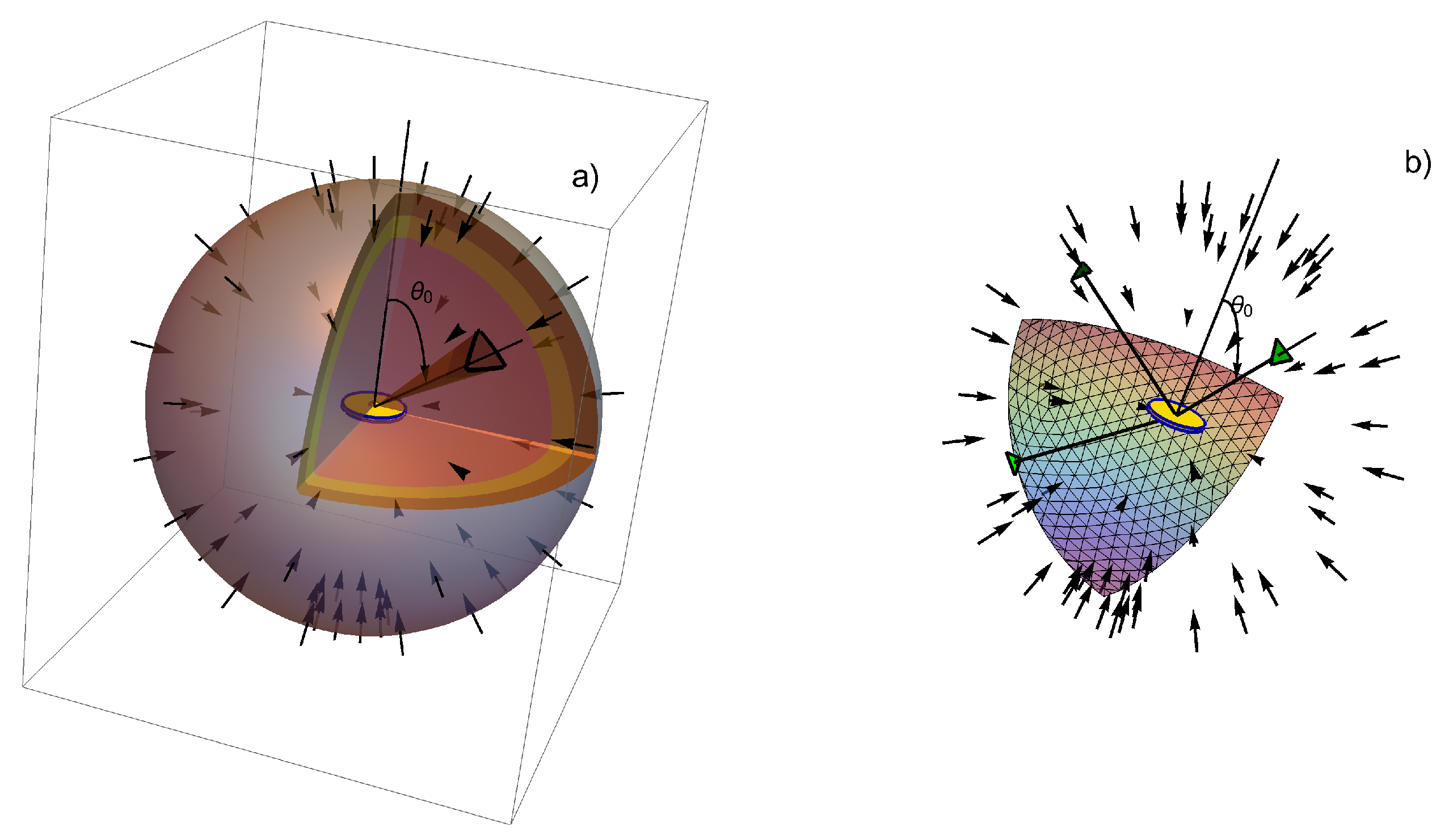
2. Non-Isothermal Radial Bondi Accretion

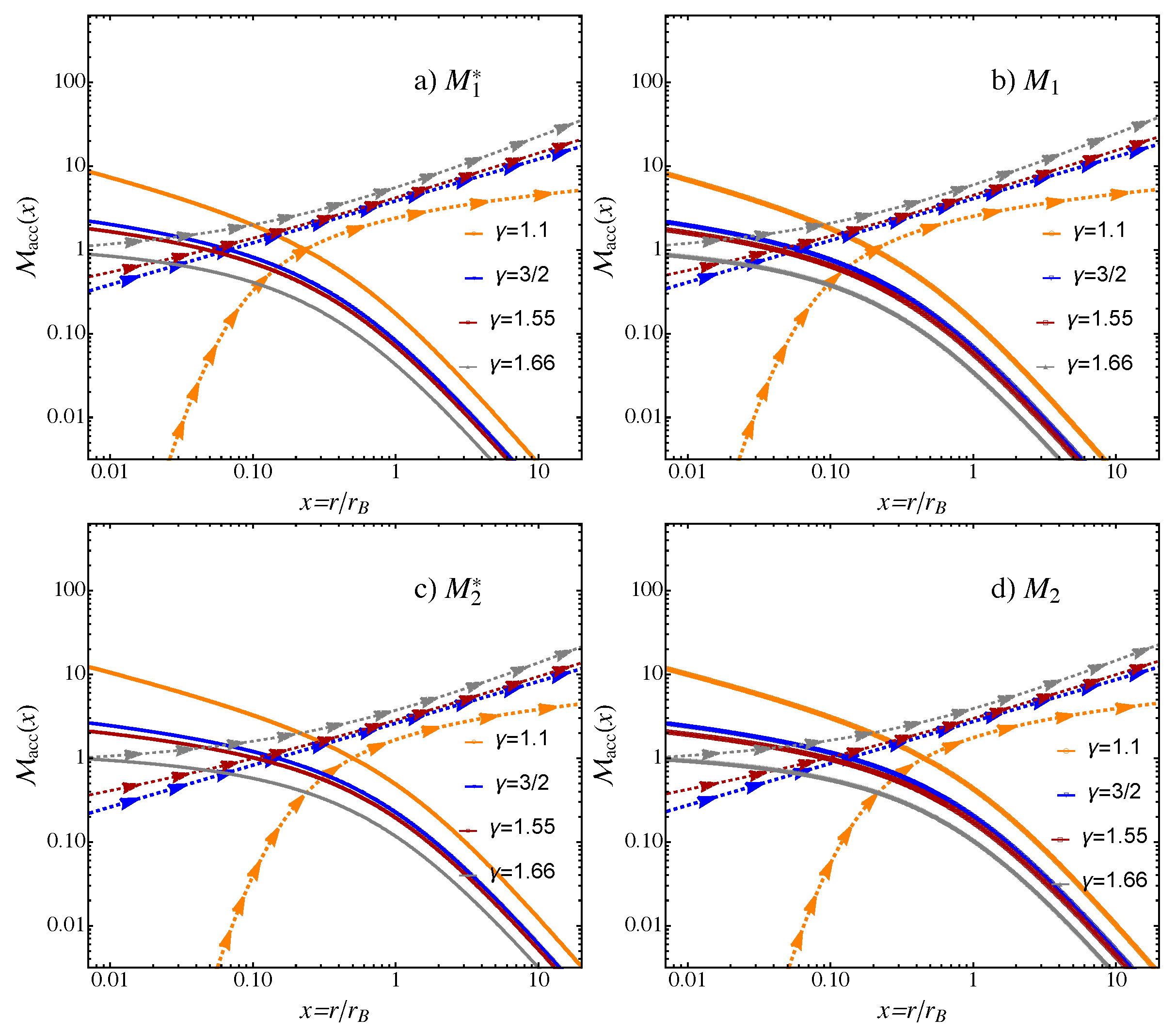
Under the effects of irradiation by X rays, the accretion flow onto the central SMBH is described by the mass and momentum conservation laws

$$\begin{array}{ccc}\hfill \frac{d\rho }{dt}& =& -\rho \nabla ·\mathbf{v},\hfill \end{array}$$

(1)

$$\begin{array}{ccc}\hfill \frac{d\mathbf{v}}{dt}& =& -\frac{1}{\rho }\nabla p+\mathbf{g}+{\mathbf{F}}^{\mathrm{rad}},\hfill \end{array}$$

(2)

where $\rho$ denotes the density, $\mathbf{v}$ the velocity field, p the gas pressure, $\mathbf{g}$ the gravitational acceleration due to the SMBH, ${\mathbf{F}}^{\mathrm{rad}}=(F_r,F_{\theta }=0,F_{\varphi }=0)$ the radiation force per unit mass, and $d/dt=\partial /\partial t+\mathbf{v}·\nabla$ the material time derivative. Using spherical coordinates and assuming that the angular components of the velocity vanish (i.e., $v_{\theta }=v_{\varphi }=0$), Equation (2) can be written as

$$\frac{\partial v_r}{\partial t}+v_r\frac{\partial v_r}{\partial r}=-\frac{1}{\rho }\frac{\partial p}{\partial r}-\frac{\partial }{\partial r}{\psi }_{\mathrm{grav}}\left(r\right)+\frac{\partial }{\partial r}{\psi }_{\mathrm{rad}}\left(r\right),$$

(3)

for the radial velocity component, where $v_r=v_r(r,\theta ,\varphi )$, $p=p(r,\theta ,\varphi )$, $M_{\mathrm{BH}}$ is the mass of the SMBH, and ${\psi }_{\mathrm{rad}}\left(r\right)$ is a function defined below. If we further assume azimuthal symmetry (i.e., $\partial /\partial \varphi =0$) and perform the analysis for a fixed angle ${\theta }_0$, such that $v_r(r,\theta ,\varphi )=v_r(r,{\theta }_0)=v_r$ and $p(r,\theta ,\varphi )=p(r,{\theta }_0)=p$, the above equation becomes

$$\frac{d\mathcal{H}\left(r\right)}{dr}=p\frac{d}{dr}\left(\frac{1}{\rho }\right)-\frac{\partial v_r}{\partial t},$$

(4)

where

$$\mathcal{H}\left(r\right)=\frac{p}{\rho }+\frac{1}{2}{v}_r^2-{\psi }_{\mathrm{grav}}\left(r\right)-{\psi }_{\mathrm{rad}}\left(r\right),$$

(5)

is the Bernoulli function $\mathcal{H}\left(r\right)$, ${\psi }_{\mathrm{grav}}=\left(G{M}_{\mathrm{BH}}\right)/r$ and ${\psi }_{\mathrm{rad}}=-C\left(r\right)/r$ are the gravitational and radiation potentials, respectively. Compared to the analysis of [38], a radial dependence is now assumed for the term C in the definition of the radiation potential. For simplicity the accretion disc is assumed to be flat, Keplerian, geometrically thin and optically thick. The pressure is related to the density by means of an ideal equation of state

$$p=\frac{k_B\rho T}{\mu m_p}=p_{\infty }{\tilde{\rho }}^{\gamma },$$

(6)

where $k_B$ is the Boltzmann constant, T is the gas temperature, $\mu$ is the mean molecular weight, and $m_p$ is the proton mass. Here $\gamma$ is varied in the range $1\le \gamma <5/3$ and $\tilde{\rho }\equiv \rho /{\rho }_{\infty }$, where $p_{\infty }$ and ${\rho }_{\infty }$ are the values of the pressure and density at infinity, respectively. The sound speed is defined according to

$$c_{\mathrm{s}}^2=\frac{\gamma p}{\rho }.$$

(7)

The radiative contributions in Equations (2) and (4) are here implemented using the strategies used by [13,39,40,41] (hereafter P07). Although the radiation field from both the disc and the central black hole are modelled as in P07 by adding a radiation force in the momentum equation, there are important differences with P07 that are worth commenting. For instance, in P07 the analysis is based on time-dependent, axisymmetric simulations with $\gamma =5/3$, while our analysis consists of steady-state calculations along radial streamlines for fixed $\theta$ and varying values of the adiabatic index in the interval $1\lesssim \gamma <5/3$. These calculations have been designed to serve as initial conditions for fully three-dimensional simulations of accretion discs [42]. As in P07, the disc is assumed to emit only UV light (i.e., $f_{\mathrm{disc}}=f_{\mathrm{UV}}$) and the central SMBH to emit only X-rays (i.e., $f_{\star }=f_{\mathrm{X}}=1-f_{\mathrm{disc}}$) so that the disc and central luminosities are given by $L_{\mathrm{disc}}=f_{\mathrm{disc}}L$ and $L_{\star }=f_{\star }L$, respectively, where L is the total accretion luminosity. The radial component of the radiation force is approximated according to the relation (e.g., P07)

$$F_{r_{\mathrm{rad}}}(r,{\theta }_0)=\frac{{\sigma }_{T}L}{4\pi r^{2}c{m}_p}\left[f_{\star }+2cos{\theta }_0{f}_{\mathrm{disk}}(1+M(r,t))\right],$$

(8)

where c is the speed of light in vacuum, ${\sigma }_T/m_p$ is the mass scattering coefficient for free electrons, ${\theta }_0$ is some fixed and constant polar angle measured from the rotational axis of the disk, and t is the optical depth

$$t=\frac{({\sigma }_T/m_p)\rho v_{\mathrm{th}}}{|d{v}_r/dr|},$$

(9)

where $v_{\mathrm{th}}$ is the thermal velocity (set using a temperature of 25,000 K), $d{v}_r/dr$ is the velocity gradient along the radial direction, and $M(r,t)$ is the so-called force multiplier [43], defined by

$$M(r,t)=k{t}^{-\alpha }\left[\frac{{(1+{\tau }_{\max })}^{(1-\alpha )}-1}{{\tau }_{\max }^{(1-\alpha )}}\right],$$

(10)

where $\alpha =0.6$ is the ratio of optically thick to optically thin lines. According to [44], the parameter k is given by the minimun between

$$k=0.03+0.385exp\left(-1.4{\xi }^{0.6}\right),$$

(11)

and

$$logk=\left\{\begin{array}{cc}-0.383,\hfill & \hfill \mathrm{for}logT\le 4,\\ -0.630logT+2.138,\hfill & \hfill \mathrm{for} 4<logT\le 4.75,\\ -0.870logT+17.528,\hfill & \hfill \mathrm{for}logT>4.75,\end{array}\right.$$

(12)

which is based on detailed photoionization calculations performed using the XSTAR code (P07), while ${\tau }_{\max }=t{\eta }_{\max }$ with

$$log{\eta }_{\max }=\left\{\begin{array}{cc}6.9exp\left(0.16{\xi }^{0.4}\right),\hfill & \hfill \mathrm{if}log\xi \le 0.5,\\ 9.1exp\left(-7.96\times {10}^{-3}\xi \right),\hfill & \hfill \mathrm{if}log\xi >0.5,\end{array}\right.$$

(13)

where $\xi$ is the photoionization parameter. The parameter ${\eta }_{\max }$ defined by Equation (13) is used to determined the maximum force multiplier, i.e., $M_{\max }=k(1-\alpha ){\eta }_{\max }^{\alpha }$. The local X-ray flux

$${\mathcal{F}}_X=\frac{L_{\star }}{4\pi r^2}exp\left(-{\tau }_X\right),$$

(14)

is used to estimate the photoionization parameter $\xi =4\pi {\mathcal{F}}_X/n$, where

$${\tau }_X={\int }_0^r{\kappa }_X\rho dr,$$

(15)

is the X-ray optical depth, evaluated between the centre ($r=0$) and a radius r in the accreting flow, and $n=\rho /\left(\mu m_p\right)$ is the number density of the accreting gas. The absorption coefficient ${\kappa }_X$ is set to 0.4 g⁻¹ cm${}^2$ for all values of $\xi$.

The $\gamma =5/3$ regime of non-isothermal Bondi accretion is modelled using the Paczyński–Wiita (PW) potential [45,46]

$${\psi }_{\mathrm{grav}}=\frac{G{M}_{\mathrm{BH}}}{r-R_s},$$

(16)

where $R_s=2G{M}_{\mathrm{BH}}/c^2$ is the gravitational radius of the black hole. While this pseudo-Newtonian potential does not obey the Poisson equation, it has become a standard tool because it accurately models the general relativistic accretion of matter onto a nonrotating SMBH. In particular, this form of the potential reproduces the radii of a marginally stable Keplerian orbit ($r=3R_s$) and of a marginally bound orbit ($r=2R_s$) as predicted by Einstein’s gravity in the Schwarzschild metric [46].

Under the assumption of steady-state motion, Equations (4) and (5) can be combined to produce after a few algebraic steps the integral equation

$$\int \frac{d}{dr}\left(\frac{{\mathcal{M}}^2{\widetilde{c_{\mathrm{s}}}}^2}{2}+\frac{{\tilde{\rho }}^{(\gamma -1)}}{\gamma -1}-\frac{1}{x}+\frac{l_{\mathrm{tot}}^{\mathrm{rad}}{|}_{\theta ={\theta }_0}\left(x\right)}{x}\right)dr=0,$$

(17)

where

$$x\equiv \frac{r}{r_B},\widetilde{c_{\mathrm{s}}}\equiv \frac{c_{\mathrm{s}}}{c_{\infty }}={\tilde{\rho }}^{(\gamma -1)/2},\mathcal{M}\equiv \frac{v_r}{c_{\mathrm{s}}},$$

(18)

and

$$l_{\mathrm{tot}}^{\mathrm{rad}}{{|}_{\theta ={\theta }_0}\left(x\right)=l_{\mathrm{Edd}}^{\mathrm{rad}}{f}_{\mathrm{rad}}|}_{\theta ={\theta }_0}\left(x\right).$$

(19)

Here ${C|}_{\theta ={\theta }_0}\left(x\right)=G{M}_{\mathrm{BH}}{l}_{\mathrm{tot}}^{\mathrm{rad}}{|}_{\theta ={\theta }_0}\left(x\right)$,

$$r_B=\frac{G{M}_{\mathrm{BH}}}{c_{\infty }^2},$$

(20)

is the Bondi radius, $c_{\infty }^2=\gamma p_{\infty }/{\rho }_{\infty }$, $\mathcal{M}$ is the Mach number, $l_{\mathrm{Edd}}^{\mathrm{rad}}=L/L_{\mathrm{Edd}}$ with $L_{\mathrm{Edd}}=4\pi cG{M}_{\mathrm{BH}}{m}_p/{\sigma }_T$ being the Eddington luminosity, ${\sigma }_T=6.6524\times {10}^{-25}$ cm${}^2$ is the Thomson cross section, and $f_{\mathrm{rad}}{|}_{\theta ={\theta }_0}\left(x\right)$ is the radiative force parameter given by the relation

$$f_{\mathrm{rad}}{|}_{\theta ={\theta }_0}\left(x\right)=f_{\star }+2cos{\theta }_0{f}_{\mathrm{disk}}[1+M(x,t)].$$

(21)

Although the force multiplier is an explicit function of x and t, for simplicity hereafter we omit the x-dependence and write it as $M(t=\tau )$.

Equation (17) can be integrated to give

$${\tilde{\rho }}^{(\gamma -1)}\left(\frac{{\mathcal{M}}^2}{2}+\frac{1}{\gamma -1}\right)=\frac{1}{x}-\frac{l_{\mathrm{tot}}^{\mathrm{rad}}{|}_{\theta ={\theta }_0}\left(x\right)}{x}+\frac{1}{\gamma -1}.$$

(22)

This equation describes the non-isothermal ($\gamma >1$), steady-state accretion along a radial streamline for a fixed angle $\theta ={\theta }_0$ when the effects of radiation emission due to electron scattering and spectral discrete lines with appropriate boundary conditions at infinity and ionization changes due to temperature corrections are considered. A sketch showing the geometry of the system is displayed in Figure 1, where a radial streamline at a meridional angle ${\theta }_0$ is shown. In terms of the above assumptions and the normalized parameters (18), Equation (1) becomes

$$x^2\mathcal{M}{\tilde{\rho }}^{(\gamma +1)/2}=\lambda ,$$

(23)

where $\lambda$ is the accretion parameter given by

$$\lambda =\frac{{\dot{M}}_B}{\left(4\pi f_{\mathrm{solid}}\right)r_B^2{\rho }_{\infty }{c}_{\infty }},$$

(24)

which determines the accretion rate for given boundary conditions and mass of the SMBH. In this expression, $4\pi f_{\mathrm{solid}}=\int sin\theta d\theta d\varphi$ is the solid angle covered by the streamline at the polar angle ${\theta }_0$ (see Figure 1). When $f_{\mathrm{solid}}=1$ (full solid angle), Equation (24) reduces to the classical accretion parameter. However, for a ${\theta }_0$-dependent force $f_{\mathrm{solid}}<<1$. This dependence is important only for the final calculation of ${\dot{M}}_B=\lambda \left(4\pi f_{\mathrm{solid}}\right)r_B^2{\rho }_{\infty }{c}_{\infty }$, which is fixed once the value of ${\theta }_0$ is chosen. Replacing $\tilde{\rho }$ from Equation (23) into Equation (22), the radiative-radial Bondi problem reduces to solving the equation

$$g\left(\mathcal{M}\right)=\Lambda f\left(x\right),\mathrm{with}\Lambda ={\lambda }^{2(1-\gamma )/(\gamma +1)},$$

(25)

where ${\chi }_{\mathrm{tot}}^{\mathrm{rad}}{{|}_{\theta ={\theta }_0}=1-l_{\mathrm{tot}}^{\mathrm{rad}}|}_{\theta ={\theta }_0}$, $\lambda ={\chi }_{\mathrm{tot}}^{\mathrm{rad}}{|}_{\theta ={\theta }_0}^2{\lambda }_{\mathrm{cr}}$, and

$$\begin{array}{ccc}\hfill g\left(\mathcal{M}\right)& =& {\mathcal{M}}^{2(1-\gamma )/(\gamma +1)}\left(\frac{{\mathcal{M}}^2}{2}+\frac{1}{\gamma -1}\right),\hfill \end{array}$$

(26)

$$\begin{array}{ccc}\hfill f\left(x\right)& =& x^{4(\gamma -1)/(\gamma +1)}\left(\frac{{\chi }_{\mathrm{tot}}^{\mathrm{rad}}{|}_{\theta ={\theta }_0}}{x}+\frac{1}{\gamma -1}\right),\hfill \end{array}$$

(27)

$$\begin{array}{ccc}\hfill {\lambda }_{\mathrm{cr}}& =& \frac{1}{4}{\left(\frac{2}{5-3\gamma }\right)}^{(5-3\gamma )/\left[2\right(\gamma -1\left)\right]}.\hfill \end{array}$$

(28)

For this case Equations (17)–(27) remain the same with the only change being the substitution of x by $x-x_s$, where $x_s=R_s/r_B$. Here we take $R_s/r_B=1.75\times {10}^{-5}$ for the calculations of Figure 2 and $2.18\times {10}^{-6}$ for the rest of the calculations. The radiative Bondi-like problem then reduces to solving Equations (25)–(28) for the Mach number, $\mathcal{M}$, as a function of radius. On the other hand, it must be noticed that the PW potential, in addition to reproducing the innermost stable circular orbit and the marginally bound orbit, also accounts for a non-vanishing critical radius for $\gamma =5/3$, in contrast to the purely Newtonian radial accretion, for which

$$x_{\mathrm{crit}}=x_s+\sqrt{\frac{2{\chi }_{\mathrm{total}}^{\mathrm{rad}}{x}_s}{3}},$$

(29)

where now the factor ${\chi }_{\mathrm{total}}^{\mathrm{rad}}$ (>0) appears, which is not present in [38,47].

The angular variation of the UV emission, ${\chi }_{\mathrm{tot}}^{\mathrm{rad}}$, for models with and without the force multiplier is shown in the top panel of Figure 2. Model $M_1$ has $f_{\star }=0.5$ and $f_{\mathrm{disc}}=0.5$, model $M_2$ has $f_{\star }=0.2$ and $f_{\mathrm{disc}}=0.8$, while model $M_3$ has $f_{\star }=0.05$ and $f_{\mathrm{disc}}=0.95$, with $M\left(\tau \right)=0$ so that both types of radiation can be evaluated in detail. Models $M_1^{\star }$, $M_2^{\star }$, and $M_3^{\star }$ differ from the preceding models in that $M\left(\tau \right)\ne 0$. For different fractions of $f_{\star }$, $f_{\mathrm{disc}}$, and position x, we estimate the critical angles for which a transition from type 5 to type 1 and 2 solutions is allowed1. This plot, which corresponds to $\tilde{\rho }=0.001$, $x=3$, and $\gamma =1.55$, is an example of the complexity of the system. In particular, $M_2^{\star }$ (green line with empty squares) and $M_3^{\star }$ (red line with full triangles) have physical transonic solutions for $\theta >\pi /8$, while model $M_1^{\star }$ (blue line with empty circles) does not admit solutions for which ${\chi }_{\mathrm{tot}}^{\mathrm{rad}}<0$, and so this flow can be seen in any angular direction. The transition for $M_2^{\star }$ occurs at a lower angle than for $M_3^{\star }$, meaning that we should find more collimated streamlines for the $M_2^{\star }$ flows than for the $M_3^{\star }$ flows. It is interesting to see that model $M_1$, for which only electron scattering is present ($M\left(\tau \right)=0$) and $f_{\star }=f_{\mathrm{disc}}=0.5$, behaves like model $M_1^{\star }$ with no transition to the unphysical region where ${\chi }_{\mathrm{tot}}^{\mathrm{rad}}<0$. As the fraction of disc photons increases (i.e., from $f_{\mathrm{disc}}=0.8$ to 0.95), critical angles for which unphysical type 5 solutions occur (for ${\theta }_{M_{2,3}}^{\mathrm{phase}}<\pi /8$) are found even when only electron scattering is dominating.

In both sets of models $M_{1,2,3}$ and $M_{1,2,3}^{\star }$, the radiation acceleration depends on the ionization parameter defined as

$$\xi =\frac{\left(f_{\star }L\right)exp(-{\tau }_X)}{n{r}^2},$$

(30)

where $L=7.45\times {10}^{45}$ erg s${}^{-1}$, which is appropriate for a ${10}^8{M}_{\odot }$ SMBH accreting at an efficiency of 8%. The gas density is $n\left(x\right)=\left({\rho }_{\infty }\tilde{\rho }\left(x\right)\right)/\left(\mu m_p\right)$ cm${}^{-3}$, with ${\rho }_{\infty }={10}^{-20}$ gr cm${}^{-3}$, $\mu =0.7$, and the optical depth ${\tau }_X$ is integrated using Equation (15) with ${\kappa }_X=0.4$ g${}^{-1}$ cm${}^2$. The physical parameters for all models computed in this study are listed in

Table 1. Parameters of the accretion models.

Run	Lines ${}^{\left(\mathbf{a}\right)}$	${\mathit{f}}_{\star }$	${\mathit{f}}_{\mathbf{disc}}$	$\mathit{\gamma }{}^{\left(\mathbf{b}\right)}$	${\mathit{\theta }}^{\mathbf{phase}}$${}^{\left(\mathbf{c}\right)}$	${\mathit{\theta }}_{\mathbf{acc}}^{\mathbf{phase}}$
					(rad)	(rad)
M${}_1^{\star }$	yes	0.50	0.50	-	$\frac{3}{8}\pi$	1.1
M${}_2^{\star }$	yes	0.20	0.80	-	$\frac{3}{8}\pi$	1.6
M${}_3^{\star }$	yes	0.05	0.95	-	$\frac{3}{8}\pi$	1.7
M${}_1$	no	0.50	0.50	-	$\frac{3}{8}\pi$	1
M${}_2$	no	0.20	0.80	-	$\frac{3}{8}\pi$	1.5
M${}_3$	no	0.05	0.95	-	$\frac{3}{8}\pi$	1.6

${}^{\left(\mathrm{a}\right)}$$M\left(t\right)\ne 0$ (yes) and $M\left(t\right)=0$ (no). ${}^{\left(\mathrm{b}\right)}$ The values of $\gamma =\{1.1,1.2,1.3,13/9,3/2,1.53,1.55,1.63,1.65,1.66\}$. ${}^{\left(\mathrm{c}\right)}$ The angle ${\theta }_{\mathrm{acc}}^{\mathrm{phase}}$ is given in terms of ${\theta }^{\mathrm{phase}}$, i.e., ${\theta }_{\mathrm{acc}}^{\mathrm{phase}}=1.1{\theta }^{\mathrm{phase}}$. All models $M_{*}^{\star }$ and $M_{*}$ shared the same angle.

(a full analysis of the angular dependence is beyond the scope of the present work, and will be presented in a forthcoming paper). In all cases we choose ${\theta }_0={\theta }_{\mathrm{acc}}^{\mathrm{phase}}$. The fractions $f_{\star }$ and $f_{\mathrm{disc}}$ in Table 1 are exactly the same used by P07, which comply with observational results from [49,50].

The bottom panel of Figure 2 shows the dependence of the Mach number of the inflow and outflow transonic solutions with the normalized radial distance from the black hole for model $M_1^{\star }$ and various characteristic values of the adiabatic index, namely $\gamma =1$ (full analytical solution; orange curves), $\gamma =1.1$ (numerical solution from [38] with ${\psi }_{\mathrm{rad}}=-C/r$; gray curves, and this paper with ${\psi }_{\mathrm{rad}}=-C\left(r\right)/r$; green curves), $\gamma =3/2$ (blue curves), $\gamma =1.55$ (black curves), $\gamma =1.66$ (magenta curves), and $\gamma =5/3$ (red curves). Note that the latter curves correspond to the PW model with no radiation, i.e., with $f_{\star }=f_{\mathrm{disc}}=0$. The intersection of curves of the same colour define the position of the sonic point ($x_s$). The thick solid curves for $x<x_s$ represent supersonic inflow solutions, while those at larger radii (i.e., $x>x_s$) represent supersonic outflow solutions. The dashed curves at radii $x>x_s$ are subsonic inflow solutions and those for $x<x_s$ are subsonic outflow solutions. The Mach number profiles are shown up to radial distances of ≈${10}^{-3.1}{r}_B$ from the centre. It is evident from this figure that isothermal ($\gamma =1$) inflow occurs at slightly higher values of ${\mathcal{M}}_{\mathrm{acc}}\left(r\right)$ than its non-isothermal counterparts. As the adiabatic index is increased the accretion rate occurs at relatively smaller values of the Mach number everywhere and closer to the central source so that the region of supersonic accretion involves progressively smaller central volumes as $\gamma$ increases. In contrast, the isothermal outflow takes place at much lower Mach numbers compared to the non-isothermal cases. These differences are clearly expected to influence the rates for non-isothermal accretion. As the adiabatic index is increased above $\gamma =3/2$ the outflow close to $x={10}^{-3}$ becomes supersonic only when $\gamma =1.66$ and keeps subsonic for all values <1.66. In the interval $0.01\lesssim x\lesssim 0.1$, the outflow proceeds supersonically for all non-isothermal cases ($\gamma >1$) with a small dependence of the Mach number on $\gamma$, while towards larger x(≳0.2) the outflow becomes more supersonic as the adiabatic index is increased.

3. Results

The Mach number as a function of distance from the source is shown in the top panel of Figure 3 for model $M_1^{\star }$ and varied $\gamma$. The solid curves depict the inflow solutions, while the dotted lines with arrows correspond to the outflow solutions. In all cases, the complete subsonic and supersonic solutions are shown. The position of the sonic point, $x_{\mathrm{crit}}$, is defined by the intersection between the inflow and the outflow solutions. When matching the subsonic portion of the solution at $x\le x_{\mathrm{crit}}$ with the supersonic one at $x>x_{\mathrm{crit}}$, we then obtain the “Bondi-outflow” solution. The difference with the Parker solution is the location of the integration limits in the Bernoulli equation. In the Bondi problem they are located at infinity, while in the Parker problem they are located at the base of the wind. For all models, the Bondi outflows are always depicted by dotted lines with small arrows pointing out of the system. On the other hand, when matching the subsonic part of the solution at $x>x_{\mathrm{crit}}$ with the supersonic one at $x\le x_{\mathrm{crit}}$, we then obtain the “Bondi-inflow” solution. Increased values of $\gamma$ produce slower inflows and faster outflows everywhere, while the position of the sonic point is shifted towards smaller radii. The left panel of Figure 4 shows a close comparison of the Mach number profiles between the Newtonian $\gamma =1.66$ case with spectral line forces (gray curves) and the $\gamma =5/3$ case with $M\left(\tau \right)=0$ (orange curves). For $M\left(\tau \right)\ne 0$ the inflow and outflow Mach number profiles essentially overlap those for the Newtonian $\gamma =1.66$ case with $M\left(\tau \right)\ne 0$ regardless of the radiation field. In spite of differences in the value of $M\left(\tau \right)$, the inflow and outflow profiles for both cases look almost identical.

Figure 3 (right panel) displays the Mach number as a function of radius for model $M_2^{\star }$ and varied $\gamma$. Compared to the left panel of Figure 3, we see that increasing the fraction of UV emission (from $f_{\star }=0.5$ to 0.2) increases the inflow Mach number everywhere, while the position of the sonic point is shifted towards larger radii. Consequently, for given $\gamma$, when the ionizing flux decreases faster inflows are produced everywhere. In particular, at small radii $x\lesssim 0.01$ the inflow becomes more supersonic. A similar trend is observed for model $M_3^{\star }$ with the weakest X-ray heating ($f_{\star }=0.05$) and the strongest UV emission ($f_{\mathrm{disc}}=0.95$), where the sonic point is moved farther away compared to model $M_2^{\star }$ and therefore the supersonic inflow close to the centre occupies a larger volume. A comparison of the right panel of Figure 4 with that of left panel shows that as the UV heating dominates over the X-ray luminosity, the ($\gamma =5/3$) inflow becomes faster than the $\gamma =1.66-M_1^{\star }$ inflow. It is interesting to note that the increase of the UV emission from $f_{\mathrm{disc}}=0.8$ to $f_{\mathrm{disc}}=0.95$ has only mild effects on the inflow and outflow Mach number profiles as well. The Mach number profiles for models $M_1$ and $M_2$ with no force multiplier (i.e., $M\left(\tau \right)=0$) and varied $\gamma$ are now displayed in Figure 3 (right), respectively. The profiles for model $M_3$ are very similar to those shown in Figure 3 for model $M_2$. For model $M_1$, where the central X-ray heating is the strongest and no line driving is present, the solution does not admit type 5 flows regardless of the incident angle. As shown in Figure 3 (bottom) the critical points occur far from the central source between $x\approx 0.2$ (for $\gamma =1.1$) and $x\approx 0.007$ (for $\gamma =1.66$). These distances are relatively similar to those found for model $M_1^{\star }$ with force multiplier. For ${\theta }_0=\frac{3}{8}\pi$ and close to the SMBH ($x\approx {10}^{-3}$), the Mach number ranges from ≈1 (for $\gamma =1.66$) to ≈8 (for $\gamma =1.1$). When the fraction of UV emission is increased to $f_{\mathrm{disc}}=0.8$, the position of the sonic point is shifted outwards so that the flow becomes supersonic in a larger central volume as can be seen by comparing bottom with top. However, model $M_2$ is characterized by smaller supersonic volumes than model $M_3$. Similarly to the cases with force multiplier, as the UV emission is increased, the flow close to the central black hole becomes more supersonic. Moreover, for $\gamma =1.66$ models $M_2$ and $M_3$ both exhibit outflows that are slower at large radii ($x>1$) than their Bondi-inflow counterparts close to the central source, while the inverse is seen to occur for larger $\gamma$.

For all models the density profiles are similar and almost independent of the adiabatic index. In all cases the density increases for $x\lesssim 0.1$ from ≈(1−7) to values as high as ≈${10}^3$ when the UV emission rises from $f_{\mathrm{disc}}=0.5$ to $f_{\mathrm{disc}}=0.95$ for models with $M\left(\tau \right)\ne 0$. In contrast, when $M\left(\tau \right)=0$ the highest central densities are seen to occur for model $M_1$ with $\tilde{\rho }\approx 5\times {10}^2$ at $x={10}^{-3}$, while models $M_2$ and $M_3$ with stronger UV emission and weaker central X-ray heating reach central densities of ≈1000 at the same radial distance from the SMBH, respectively. Additionally, in these cases the density profiles show a very little dependence on the adiabatic index. It is clear from the present results that the flow dynamics are sensitive to the radiative process that dominates the environment.

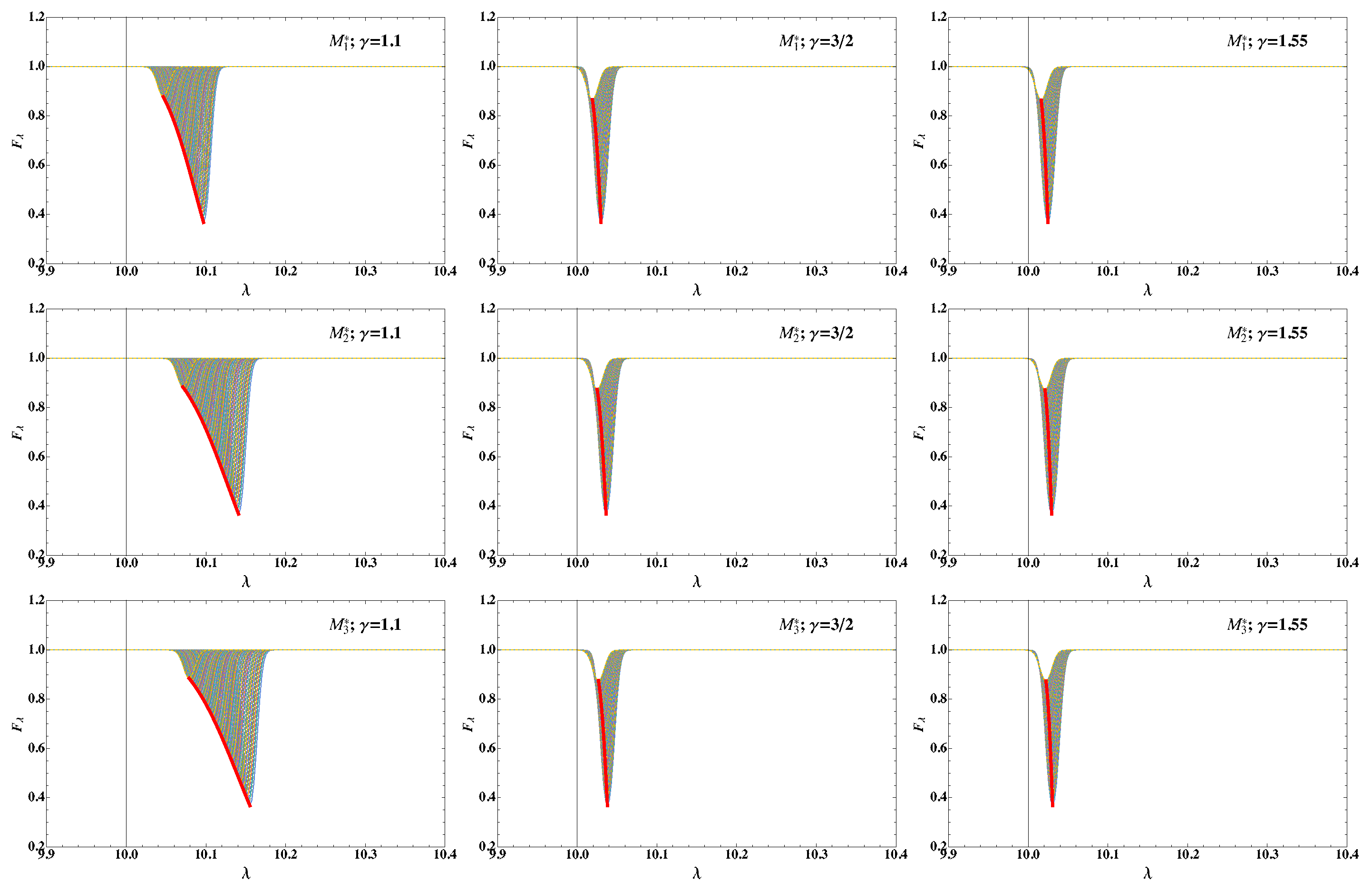
4. Catalogue of Pure Absorption Spectral Line Shapes for $\mathbf{1}.\mathbf{1}\le \mathbf{\gamma }\le \mathbf{1}.\mathbf{66}$

As resolution improves with the emergence of more powerful telescopes, it becomes mandatory to predict the shape of absorption spectral lines as seen by a distant observer. This can be done by imagining a radially falling atom onto the SMBH according to the predictions of models $M_{1,2,3}^{\star }$, which would absorb photons emitted by the inner region at 10 Å in the rest-frame. Then we use the Doppler-shift formula [51]:

$$w=\frac{w_0}{\gamma L(1-\frac{\mathrm{v}\left(x\right)}{c}cos\varphi )},$$

(31)

where w is the angular frequency of an emitted photon with rest-frame frequency $w_0$ as measured by the observer, $\gamma L$ is the Lorentz factor, $\mathrm{v}\left(x\right)$ is the velocity of the absorbing atom, and $\varphi$ is the angle between the streamline and the line-of-sight towards the observer, which we set to $\varphi =0$. For falling particles we set $\mathrm{v}\left(x\right)=-\mathcal{M}\left(x\right)c_{\mathrm{s}}$, where $c_{\mathrm{s}}$ is given by Equation (7)2, for values of ≈360, 420, 430, 440, and 420 km s${}^{-1}$. A simple description of the absorption spectrum is given by

$$F_{\lambda }\left(x\right)=exp\left\{-A\left(x\right)exp\left[-\frac{{\left(\lambda \left(x\right)-{\lambda }_0\right)}^2}{{\sigma }^2}\right]\right\},$$

(32)

where ${\nu }_0{\lambda }_0=w_0/\left(2\pi \right){\lambda }_0=c$, $\sigma$ is given by $0.1\%\lambda \left(x\right)$, c is the speed of light, and ${\lambda }_0$ is the photon wavelength in the rest frame. The intensity of the absorption is modelled by setting $A\left(x\right)=\rho \left(x\right)/{\rho }_{\max }$, where $\rho \left(x\right)=\tilde{\rho }\left(x\right){\rho }_{\infty }$ and ${\rho }_{\max }=\tilde{\rho }(x=3\times {10}^{-4}){\rho }_{\infty }$. As the particle is getting closer and closer to the black hole, the density increases and the shape of the spectral line tends to have a deeper deep shifted towards the red. Figure 5 depicts the predicted accretion absorption line shape for models $M_1^{\star }$, $M_2^{\star }$, and $M_3^{\star }$ with varied values of $\gamma$. From this figure, it is clear that the most asymmetrical lines are for model $M_3^{\star }$ corresponding to $f_{\star }=0.05$, for which the high-energy radiation is weaker making the particle to attain higher velocities and therefore more asymmetry. Telescopes with higher resolutions will be needed to resolve the asymmetry of these lines. As the UV emission dominates over the X-ray heating the absorption lines become broader, while they become narrower with increasing $\gamma$ regardless of the radiation field. For $\gamma =1.1$ the symmetry is enough to distinguish which source of radiation is dominant with a resolution of ≈2500 km s${}^{-1}$. However, as $\gamma$ increases this property is lost as changes in the fraction of UV heating from $f_{\mathrm{disc}}=0.5$ to 0.95 cannot be easily distinguished from the shape of the spectral absorption lines.

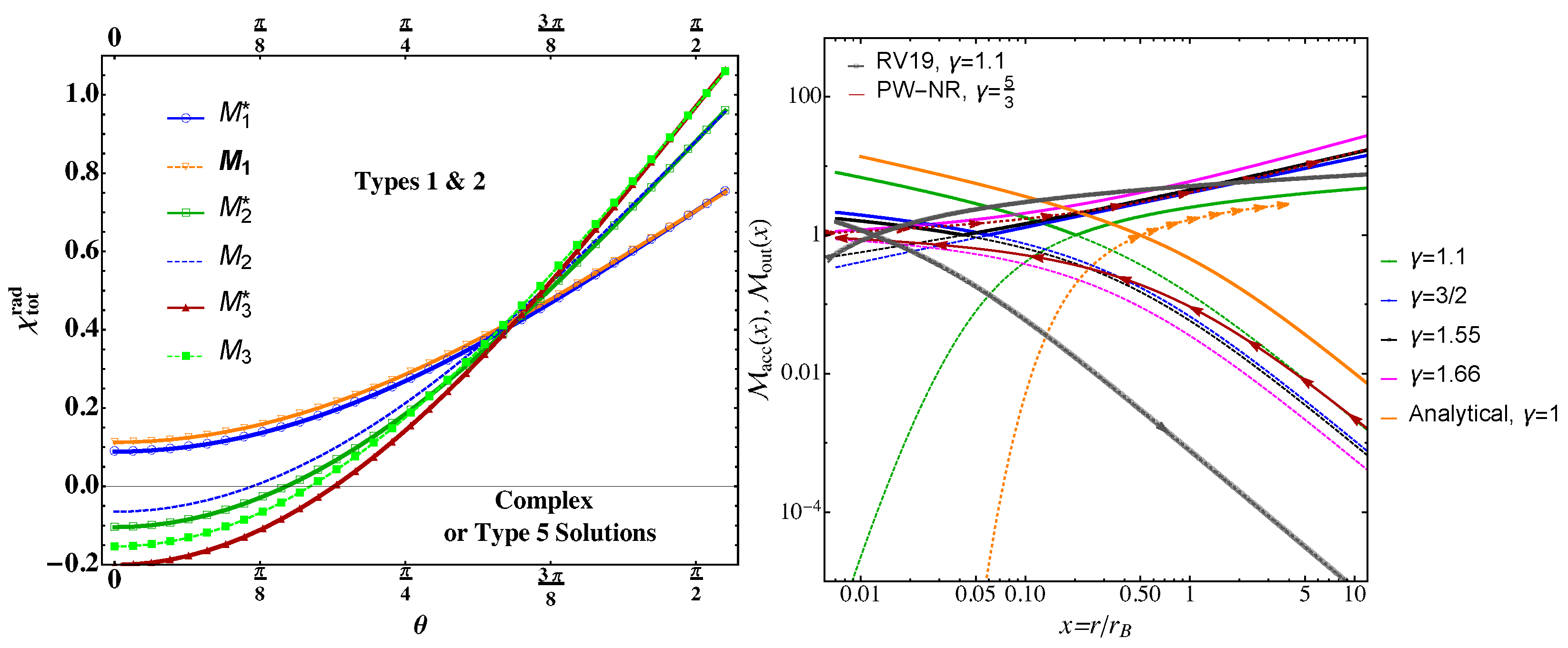
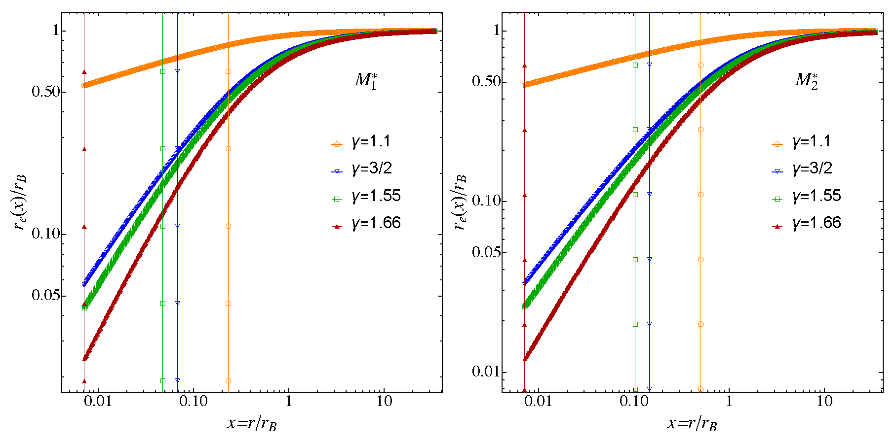
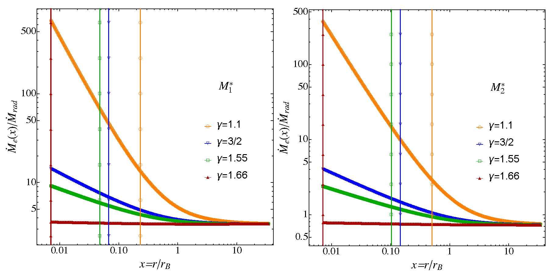
5. Estimated Bondi Radius and Mass Accretion with Respect to Conditions at Infinity

We are now in the position to quantify the ratio between the estimated ($r_e$) and the true ($r_B$) values of the Bondi radius and that between the estimated (${\dot{M}}_e$) and the true (${\dot{M}}_{\mathrm{rad}}$) accretion rates when the boundary conditions are not at infinity. These ratios are given as functions of the radial distance from the SMBH by the following relations

$$\begin{array}{ccc}\hfill \frac{r_{e;\{\mathrm{acc},\mathrm{out}\}}\left(x\right)}{r_B}& =& {\left(\frac{x^2{\mathcal{M}}_{\{\mathrm{acc},\mathrm{out}\}}}{\lambda }\right)}^{2(\gamma -1)/(\gamma +1)},\hfill \end{array}$$

(33)

$$\begin{array}{ccc}\hfill \frac{{\dot{M}}_{e;\{\mathrm{acc},\mathrm{out}\}}\left(x\right)}{{\dot{M}}_{\mathrm{rad}}}& =& \frac{1}{{\chi }_{\mathrm{tot}}^{\mathrm{rad}}{|}_{\theta ={\theta }_0}^2}{\left[\frac{r_{e;\{\mathrm{acc},\mathrm{out}\}}\left(x\right)}{r_B}\right]}^{-(5-3\gamma )/\left[2\right(\gamma -1\left)\right]},\hfill \end{array}$$

(34)

respectively, where ${\chi }_{\mathrm{tot}}^{\mathrm{rad}}(\theta ,x)$ is the angle- and space-dependent radiative factor. Figure 6 (left) shows the estimated Bondi radii for model $M_1^{\star }$ for adiabatic indices between $\gamma =1.1$ and $1.66$. At small radial distances ($x=8\times {10}^{-3}$), model $M_1^{\star }$ with $\gamma =1.1$ has an estimated Bondi radius of $r_e/r_B\approx 0.50$. As the adiabatic index is increased, the ratio $r_e/r_B$ decreases reaching values slightly less than 0.5 for $\gamma =1.1$ and as low as ≈0.03 for $\gamma =1.66$ at $x={10}^{-2}$. The same trends are also seen for models $M_2^{\star }$ (see Figure 6 (right)) and $M_3^{\star }$ as $\gamma$ is increased, except that now the estimated Bondi radii achieve slightly lower values as the radiation field is dominated by the UV emission from the accretion disc. The profiles for model $M_3^{\star }$ are very similar to those displayed in Figure 6 with the ratios $r_e/r_B$ achieving slightly smaller values close to the centre. For all models regardless of the adiabatic index the ratio $r_e/r_B\to 1$ at large radii ($x=3$).

Figure 7 shows the estimated accretion rates for models $M_1^{\star }$, and $M_2^{\star }$, for varied values of $\gamma$. When the UV emission is increased from $f_{\mathrm{disc}}=0.8$ to 0.95 for model $M_3^{\star }$ the trends are almost the same as those in Figure 7 (right) for model $M_2^{\star }$. In all cases, the radiative effects lead to an overestimation of the accretion rates for $x\lesssim 0.1$ (model $M_1^{\star }$) and $x\lesssim 0.12$ (models $M_2^{\star }$ and $M_3^{\star }$). The differences between ${\dot{M}}_e\left(x\right)$ and ${\dot{M}}_{\mathrm{rad}}$ grow rapidly as we get closer to the central source. However, the rapid growth of the ratio ${\dot{M}}_e\left(x\right)/{\dot{M}}_{\mathrm{rad}}$ towards the centre becomes progressively less steep as $\gamma$ is increased, with ${\dot{M}}_e\left(x\right)/{\dot{M}}_{\mathrm{rad}}$ becoming almost flat for $\gamma =1.66$. For instance, model $M_1^{\star }$ has an accretion rate at $x={10}^{-2}$ for $\gamma =1.1$ that is about 100 times larger than for $\gamma =1.66$. A similar difference between both values of $\gamma$ happens when comparing models $M_2^{\star }$ and $M_3^{\star }$, where the UV emission from the disc dominates over the incident X-ray flux. The observed large overestimations in the estimated accretion rates make sense because as the closer the accreting matter is to the source of gravitation, the less accurate are the determination of $\rho$ and $c_{\mathrm{s}}$ from their values at infinity. However, the authors of [38] found that the level of overestimation of the accretion rates compared to the classical Bondi problem is slightly attenuated when the effects of line driving are ignored (model $M_1$ with $\gamma =1.1$). The same is true for higher values of $\gamma$.

6. Conclusions

In this paper, we have investigated the non-isothermal Bondi accretion onto a supermassive black hole (SMBH) when the adiabatic index is varied in the interval $1.1\le \gamma \le 1.66$ by including the effects of X-ray heating and UV emission. The radiation field is modelled using the prescriptions introduced by [13] (P07), where a central SMBH is considered as a source of X-ray heating and a surrounding optically thick, geometrically thin, standard accretion disc as a source of UV radiation. The radiative, non-isothermal radial accretion is solved semi-analytically using a method similar to that developed by the authors of [41]. The X-ray heating from the SMBH is assumed to be isotropic, while the UV emission from the accretion disc is assumed to have an angular dependence. The effects of both types of radiation are studied for different flux fractions ($f_{\star }$ and $f_{\mathrm{disc}}$) and an incident angle ${\theta }_0={\theta }_{\mathrm{acc}}^{\mathrm{phase}}$ in the presence and absence of the effects of spectral line driving. The $\gamma =5/3$ regime is also explored using the Paczyński–Wiita (PW) potential for the case when the effects of line driving are ignored.

The relevant conclusions are summarized as follows:

• Mass inflows with $1.1\le \gamma \le 1.66$ occur at lower Mach numbers everywhere compared with pure isothermal ($\gamma =1$) inflows, while isothermal outflows take place at much lower Mach numbers than their non-isothermal counterparts. In addition, for the isothermal accretion the sonic radius occurs at larger distances from the centre compared to the non-isothermal inflows, implying that in the former case the supersonic flow occupies a much larger central volume.
• When the UV flux dominates over the X-ray heating in models with spectral line driving, the inflow for given $\gamma$ becomes faster everywhere. In particular, at radial distances as close as ${10}^{-3}{r}_B$ from the central source the inflow is always supersonic regardless of $\gamma$, where $r_B$ is the Bondi radius. However, as the adiabatic index is increased from $\gamma =1.1$ to $\gamma =1.66$, the inflow of matter occurs at lower Mach numbers.
• The position of the sonic point depends on both the radiation field and the adiabatic index. In particular, when line driving is allowed and $\gamma$ is increased from 1.1 to 1.66 the sonic point is at smaller radial distances from the centre. Hence, the central volume occupied by the supersonic inflow decreases in radius with increasing $\gamma$. For given $\gamma$, as the UV emission dominates over the X-ray heating the sonic point is shifted towards larger radii and, as a consequence, the supersonic inflow will occupy larger volumes.
• As long as the fraction of X-ray heating is comparable to that of UV emission from the accretion disc, the outflow at large radii from the central source becomes more supersonic than the inflow close to the black hole. Independently of the radiation field, the faster outflows always occur when $\gamma =1.66$.
• With no line driving, the inflow becomes less supersonic as the UV emission dominates over the X-ray heating and the values of $\gamma$ increases. In fact, as the UV radiation becomes stronger, the central volume occupied by the supersonic inflow becomes larger as the sonic points are shifted towards larger radii from the gravitational source. In contrast, the outflows become more supersonic as the UV emission becomes stronger and $\gamma$ is increased.
• At distances of ${10}^{-3}{r}_B$ from the central source, the ratio of the estimated to the true Bondi radius is always below one. Independently of the dominant type of radiation, the deviations between the estimated and true Bondi radius increase with increasing $\gamma$. For given $\gamma$ between $1.1$ and $1.66$, this ratio drops faster as the radiation field is dominated by the UV emission.
• Under the effects of line driving, the radiative effects lead to an overestimation of the accretion rates close to the centre. The deviation between the estimated and the true accretion rate increases with decreasing $\gamma$. For given $\gamma$, the deviation decreases as the UV emission becomes stronger.
• The models predict broader absorption lines when the UV emission dominates over the high-energy (X-ray) heating, when going from $f_{\mathrm{disk}}=0.8\to 0.95$, which in turn become narrower as the value of $\gamma$ is increased. For low $\gamma (=1.1)$ the lines are so asymmetric, e.g., [52,53], that they can be used to infer which source of radiation is dominant with resolutions of ≈3000 km s${}^{-1}$. As $\gamma$ is increased and the lines become narrower, their shape can no longer be used to distinguish the dominant source of heating.
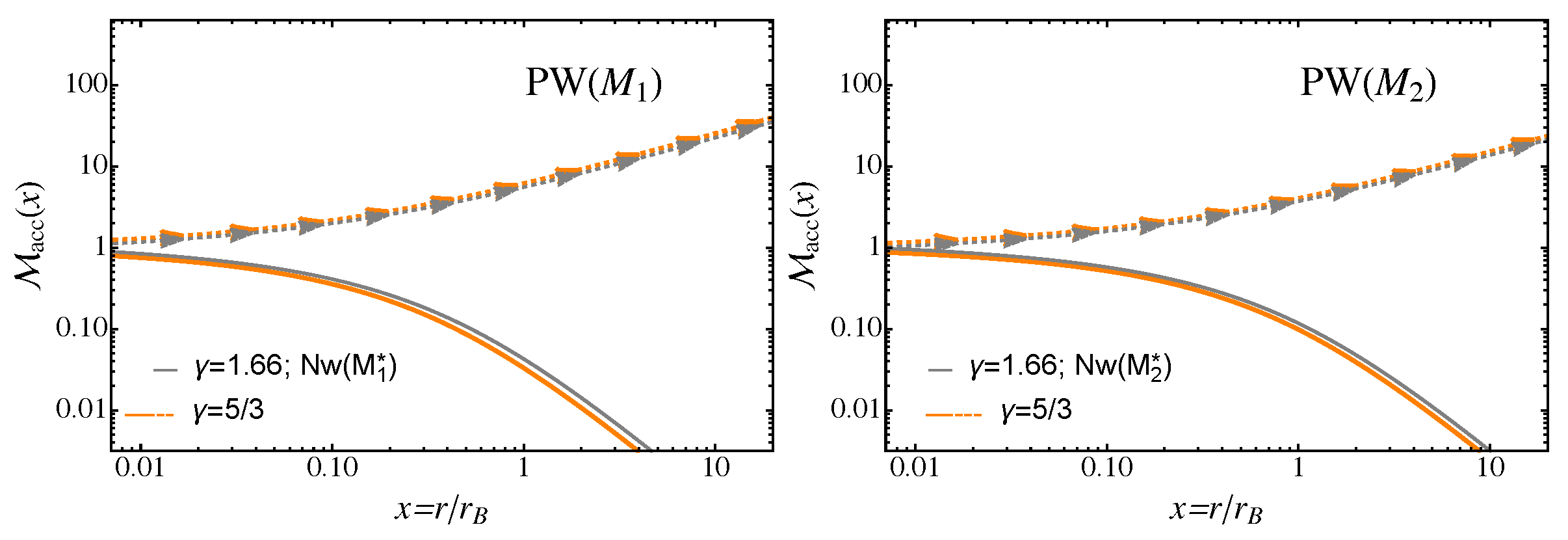
• Compared to the Newtonian $\gamma =1.66$ case, the PW model with $\gamma =5/3$ and no spectral line driving exhibits almost identical inflow Mach numbers everywhere. As the UV emission dominates over the X-ray heating, i.e., when $f_{\mathrm{disk}}$ increases from 0.5 to 0.8, both the inflow and outflow become slightly faster for the Newtonian $\gamma =1.66$ case.

References

1. Kormendy, J.; Richstone, D. Inward bound—The search for supermassive black holes in galactic nuclei. Annu. Rev. Astron. Astrophys. 1995, 33, 581–624. [Google Scholar] [CrossRef]
2. Ferrarese, L.; Ford, H. Supermassive black holes in galactic nuclei: Past, present and future research. Space Sci. Rev. 2005, 116, 523–624. [Google Scholar] [CrossRef] [Green Version]
3. Contreras, E.; Rincón, Á.; Ramírez-Velásquez, J.M. Relativistic dust accretion onto a scale-dependent polytropic black hole. Eur. Phys. J. C 2019, 79, 53. [Google Scholar] [CrossRef]
4. Bondi, H. On spherically symmetrical accretion. Mon. Not. R. Astron. Soc. 1952, 112, 195–204. [Google Scholar] [CrossRef]
5. Salpeter, E.E. Accretion of interstellar matter by massive objects. Astrophys. J. 1964, 140, 796–800. [Google Scholar] [CrossRef]
6. Fabian, A.C. The obscured growth of massive black holes. Mon. Not. R. Astron. Soc. 1999, 308, L39–L43. [Google Scholar] [CrossRef] [Green Version]
7. Barai, P. Large-scale impact of the cosmological population of expanding radio galaxies. Astrophys. J. Lett. 2008, 682, L17–L20. [Google Scholar] [CrossRef]
8. Germain, J.; Barai, P.; Martel, H. Anisotropic active galactic nucleus outflows and enrichment of the intergalactic medium. I. Metal disribution. Astrophys. J. 2009, 704, 1002–1020. [Google Scholar] [CrossRef] [Green Version]
9. Croston, J.H.; Hardcastle, M.J.; Birkinshaw, M.; Worrall, D.M.; Laing, R.A. An XMM-Newton study of the environments, particle content and impact of low-power radio galaxies. Mon. Not. R. Astron. Soc. 2008, 386, 1709–1728. [Google Scholar] [CrossRef] [Green Version]
10. DiMatteo, T.; Springel, V.; Hernquist, L. Energy input from quasars regulates the growth and activity of black holes and their host galaxies. Nature 2005, 433, 604–607. [Google Scholar] [CrossRef]
11. Sincell, M.W.; Krolik, J.H. The vertical structure and ultraviolet spectrum of X-ray-irradiated accretion disks in active galactic nuclei. Astrophys. J. 1997, 476, 605–619. [Google Scholar] [CrossRef] [Green Version]
12. Proga, D. Winds from accretion disks driven by radiation and magnetocentrifugal force. Astrophys. J. 2000, 538, 684–690. [Google Scholar] [CrossRef] [Green Version]
13. Proga, D. Dynamics of accretion flows irradiated by a quasar. Astrophys. J. 2007, 661, 693–702. [Google Scholar] [CrossRef]
14. Proga, D.; Waters, T. Cloud formation and acceleration in a radiative environment. Astrophys. J. 2015, 804, 137. [Google Scholar] [CrossRef]
15. Ramírez-Velasquez, J.M.; Klapp, J.; Gabbasov, R.; Cruz, F.; Sigalotti, L.D. Impetus: New cloudy’s radiative tables for accretion onto a galaxy black hole. Astrophys. J. Suppl. Ser. 2016, 226, 22. [Google Scholar] [CrossRef] [Green Version]
16. Dyda, S.; Dannen, R.; Waters, T.; Proga, D. Irradiation of astrophysical objects—SED and flux effects on thermally driven winds. Mon. Not. R. Astron. Soc. 2017, 467, 4161–4173. [Google Scholar] [CrossRef] [Green Version]
17. Ramírez-Velasquez, J.M.; Klapp, J.; Gabbasov, R.; Cruz, F.; Sigalotti, L.D. The IMPETUS project: Using ABACUS for the high performance computation of radiative tables for accretion onto a galaxy black hole. In Recent Developments in High Performance Computing; Barrios Hernández, C.J., Gitler, I., Klapp, J., Eds.; Springer: Berlin/Heidelberg, Germany, 2017; Volume 697, pp. 374–386. [Google Scholar]
18. Silk, J.; Rees, M.J. Quasars and galaxy formation. Astron. Astrophys. 1998, 331, L1–L4. [Google Scholar]
19. Furlanetto, S.R.; Loeb, A. Metal absorption lines as probes of the intergalactic medium prior to the reionization epoch. Astrophys. J. 2003, 588, 18–34. [Google Scholar] [CrossRef] [Green Version]
20. Haiman, Z.; Bryan, G.L. Was star formation suppressed in high-redshift minihalos? Astrophys. J. 2006, 65, 7–11. [Google Scholar] [CrossRef]
21. Hopkins, P.F.; Hernquist, L.; Cox, T.J.; Robertson, B.; Springel, V. Determining the properties and evolution of red galaxies from the quasar luminosity function. Astrophys. J. Suppl. Ser. 2006, 163, 50–79. [Google Scholar] [CrossRef] [Green Version]
22. Ciotti, L.; Ostriker, J.P.; Proga, D. Feedback from central black holes in elliptical galaxies. III. Models with both radiative and mechanical feedback. Astrophys. J. 2010, 717, 708–723. [Google Scholar] [CrossRef]
23. McCarthy, I.G.; Schaye, J.; Ponman, T.J.; Bower, R.G.; Booth, C.M.; DallaVecchia, C.; Crain, R.A.; Springel, V.; Theuns, T.; Wiersma, R.P.C. The case for AGN feedback in galaxy groups. Mon. Not. R. Astron. Soc. 2010, 406, 822–839. [Google Scholar] [CrossRef] [Green Version]
24. Ostriker, J.P.; Choi, E.; Ciotti, L.; Novak, G.S.; Proga, D. Momentum driving: Which physical processes dominate active galactic nucleus feedback? Astrophys. J. 2010, 722, 642–652. [Google Scholar] [CrossRef]
25. Fabian, A.C. Observational evidence of active galactic nuclei feefback. Annu. Rev. Astron. Astrophys. 2012, 50, 455–489. [Google Scholar] [CrossRef] [Green Version]
26. Faucher-Giguère, C.-A.; Quataert, E.; Murray, N. A physical model of FeLoBALs: Implications for quasar feedback. Mon. Not. R. Astron. Soc. 2012, 420, 1347–1353. [Google Scholar] [CrossRef] [Green Version]
27. Choi, E.; Naab, T.; Ostriker, J.P.; Johansson, P.H.; Moster, B.P. Consequences of mechaical and radiative feedback from black holes in disc galaxy mergers. Mon. Not. R. Astron. Soc. 2014, 442, 440–453. [Google Scholar] [CrossRef]
28. Dannen, R.C.; Proga, D.; Kallman, T.R.; Waters, T. Photoionization calculations of the radiation force due to spectral lines in AGNs. arXiv 2019, arXiv:1812.01773v2. [Google Scholar] [CrossRef] [Green Version]
29. Palit, I.; Janiuk, A.; Sukova, P. Effects of adiabatic index on the sonic surface and time variability of low angular momentum accretion flows. Mon. Not. R. Astron. Soc. 2019, 487, 755–768. [Google Scholar] [CrossRef] [Green Version]
30. Chakrabarti, S.K.; Das, S. Model dependence of transonic properties of accretion flows around black holes. Mon. Not. R. Astron. Soc. 2001, 327, 808–812. [Google Scholar] [CrossRef] [Green Version]
31. Das, T.K. On some transonic aspects of general relativistic spherical accretion on to Schwarzschild black holes. Mon. Not. R. Astron. Soc. 2002, 330, 563–566. [Google Scholar] [CrossRef] [Green Version]
32. Meliani, Z.; Sauty, C.; Tsinganos, K.; Vlahakis, N. Relativistic Parker winds with variable effective polytropic index. Astron. Astrophys. 2004, 425, 773–781. [Google Scholar] [CrossRef]
33. Fukue, J. Transonic disk accretion revisited. Publ. Astron. Soc. Jpn. 1987, 39, 309–327. [Google Scholar]
34. Chattopadhyay, I.; Ryu, D. Effects of fluid composition on spherical flows around black holes. Astrophys. J. 2009, 694, 492. [Google Scholar] [CrossRef]
35. Sarkar, S.; Chattopadhyay, I.; Laurent, P. Two-temperature solutions and emergent spectra from relativistic accretion discs around black holes. Astron. Astrophys. 2020, 642, A209. [Google Scholar] [CrossRef]
36. Fabian, A.C.; Rees, M.J. The accretion luminosity of a massive black hole in an elliptical galaxy. Mon. Not. R. Astron. Soc. 1995, 277, L55–L58. [Google Scholar] [CrossRef] [Green Version]
37. Volonteri, M.; Rees, M.J. Rapid growth of high-redshift black holes. Astrophys. J. 2005, 633, 624–629. [Google Scholar] [CrossRef] [Green Version]
38. Ramírez-Velasquez, J.M.; Sigalotti, L.D.; Gabbasov, R.; Klapp, J.; Contreras, E. Bondi accretion for adiabatic flows onto a massive black hole with an accretion disc. The one dimensional problem. Astron. Astrophys. 2019, 631, A13. [Google Scholar] [CrossRef]
39. Ciotti, L.; Pellegrini, S. Isothermal Bondi accretion in Jaffe and Hernquist galaxies with a central black hole: Fully analytical solutions. Astrophys. J. 2017, 848, 29. [Google Scholar] [CrossRef] [Green Version]
40. Ciotti, L.; ZiaeeLorzad, A. Two-component Jaffe models with a central black hole—I. The spherical case. Mon. Not. R. Astron. Soc. 2018, 473, 5476–5491. [Google Scholar] [CrossRef] [Green Version]
41. Korol, V.; Ciotti, L.; Pellegrini, S. Bondi accretion in early-type galaxies. Mon. Not. R. Astron. Soc. 2016, 460, 1188–1200. [Google Scholar] [CrossRef] [Green Version]
42. Ramírez-Velasquez, J.M.; Sigalotti, L.D.; Gabbasov, R.; Cruz, F.; Klapp, J. IMPETUS: Consistent SPH calculations of 3D spherical Bondi accretion on to a black hole. Mon. Not. R. Astron. Soc. 2018, 477, 4308–4329. [Google Scholar] [CrossRef] [Green Version]
43. Castor, J.I.; Abbott, D.C.; Klein, R.I. Radiation-driven winds of of stars. Astrophys. J. 1975, 195, 157–174. [Google Scholar] [CrossRef]
44. Stevens, I.R.; Kallman, T.R. X-ray illuminated stellar winds: Ionization effects in the radiative driving of stellar winds in massive X-ray binary systems. Astrophys. J. 1990, 365, 321–331. [Google Scholar] [CrossRef]
45. Paczyński, B.; Wiita, P.J. Thick accretion disks and supercritical luminosities. Astron. Astrophys. 1980, 88, 23–31. [Google Scholar]
46. Abramowicz, M.A. The Paczyński-Wiita potential. A step-by-step derivation. Astron. Astrophys. 2009, 500, 213–214. [Google Scholar] [CrossRef] [Green Version]
47. Proga, D.; Begelman, M.C. Accretion of low angular momentum material onto black holes: Two-dimensional hydrodynamical inviscid case. Astrophys. J. 2003, 582, 69–81. [Google Scholar] [CrossRef]
48. Frank, J.; King, A.; Raine, D.J. Accretion Power in Astrophysics, 3rd ed.; Cambridge University Press: Cambridge, UK, 2002. [Google Scholar]
49. Laor, A.; Fiore, F.; Elvis, M.; Wilkes, B.J.; McDowell, J.C. The soft X-ray properties of a complete sample of optically selected quasars. II. Final results. Astrophys. J. 1997, 477, 93–113. [Google Scholar] [CrossRef]
50. Zheng, W.; Kriss, G.A.; Telfer, R.C.; Grimes, J.P.; Davidsen, A.F. A composite HST spectrum of quasars. Astrophys. J. 1997, 475, 469–478. [Google Scholar] [CrossRef] [Green Version]
51. Rybicki, G.B.; Lightman, A.P. Radiative Processes in Astrophysics; Wiley-Interscience: New York, NY, USA, 1979. [Google Scholar]
52. Ramírez, J.M.; Bautista, M.; Kallman, T. Line asymmetry in the Seyfert galaxy NGC 3783. Astrophys. J. 2005, 627, 166–176. [Google Scholar] [CrossRef]
53. Ramírez, J.M. Kinematics from spectral lines for AGN outflows based on time-independent radiation-driven wind theory. Rev. Mex. Astron. Astrofísica 2011, 47, 385–399. [Google Scholar]
Figure 1. Model geometry. (a) Integration is performed along a radial streamline for a fixed meridional angle θ 0 . (b) The full angular dependence can be obtained by integrating along different radial streamlines.
Galaxies 09 00055 g001
Figure 2. (Left) Angular dependence of the UV emission for models M 1 , 2 , 3 and M 1 , 2 , 3 . The horizontal black solid line at χ tot rad = 0 mark the transition from type 5 to types 1 and 2 solutions. (Right) Mach number as a function of radius for model M 1 and γ = 1 (analytical solution; orange curves), γ = 1.1 (numerical solution from [38] with ψ rad = C / r ; gray curves, and this work with C = C ( r ) ; green curves), γ = 3 / 2 (blue curves), γ = 1.55 (black curves), γ = 1.66 (magenta curves) and γ = 5 / 3 (non-radiative (NR), with x s = 2.5 × 10 3 ; red curves). The thick solid curves represent supersonic inflow ( x < x s ) and outflow ( x > x s ) solutions, while the dashed lines represent inflow and ourflow subsonic solutions.
Galaxies 09 00055 g002
Figure 3. (Top) Radial Mach number profiles of the inflow (solid lines) and outflow (dotted lines with arrows) solutions for model (a) M 1 with M ( τ ) 0 and (b) M 1 with M ( τ ) = 0 , f = 0.5 , f disc = 0.5 , and varied γ in the interval 1.1 γ 1.66 . (Bottom) (c) M 2 with M ( τ ) 0 and (d) M 2 with M ( τ ) = 0 , f = 0.2 , f disc = 0.8 .
Galaxies 09 00055 g003
Figure 4. Comparison of the Mach number profiles between the Newtonian ( γ = 1.66 ) case with spectral line forces and the ( γ = 5 / 3 ) case with M ( τ ) = 0 .
Galaxies 09 00055 g004
Figure 5. Absorption line shapes as predicted for models M 1 , M 2 , and M 3 with varied adiabatic indices in the range 1.1 γ 1.66 . The solid red lines depict the profiles of a typical absorption line for an atom falling off onto a black hole.
Galaxies 09 00055 g005
Figure 6. (Left) Estimated Bondi radii for model M 1 with M ( τ ) 0 . (Right  M 2 with M ( τ ) 0 ), f = 0.5 ( 0.2 ) and f disc = 0.5 ( 0.8 ) for varied values of the adiabatic index in the range 1.1 γ 1.66 . The vertical solid lines mark the position of the sonic point and the symbols on them identify to which inflow solution they correspond to.
Galaxies 09 00055 g006
Figure 7. (Left) Estimated accretion rates for model M 1 with M ( τ ) 0 (Right  M 2 with M ( τ ) 0 ), f = 0.5 and f disc = 0.5 for varied values of the adiabatic index in the range 1.1 γ 1.66 . The vertical solid lines mark the position of the sonic point and the symbols on them identify to which inflow solution they correspond to.
Galaxies 09 00055 g007