Review

Quantum Cosmology in the Light of Quantum Mechanics

by
Salvador J. Robles-Pérez
1,2
1
Departamento de matemáticas, IES Miguel Delibes, Miguel Hernández 2, 28991 Torrejón de la Calzada, Spain
2
Estación Ecológica de Biocosmología, Pedro de Alvarado, 14, 06411 Medellín, Spain
Galaxies 2019, 7(2), 50; https://doi.org/10.3390/galaxies7020050
Submission received: 29 January 2019 / Revised: 10 April 2019 / Accepted: 18 April 2019 / Published: 24 April 2019

Abstract

:
There is a formal analogy between the evolution of the universe, when it is seen as a trajectory in the minisuperspace, and the worldline followed by a test particle in a curved spacetime. The analogy can be extended to the quantum realm, where the trajectories are transformed into wave packets that give us the probability of finding the universe or the particle in a given point of their respective spaces: the spacetime in the case of the particle and the minisuperspace in the case of the universe. The wave function of the spacetime and the matter fields, all together, can then be seen as a super-field that propagates in the minisuperspace and the so-called third quantisation procedure can be applied in a parallel way as the second quantisation procedure is performed with a matter field that propagates in the spacetime. The super-field can thus be interpreted as made up of universes propagating, i.e., evolving, in the minisuperspace. The analogy can also be used in the opposite direction. The way in which the semiclassical state of the universe is obtained in quantum cosmology allows us to obtain, from the quantum state of a field that propagates in the spacetime, the geodesics of the underlying spacetime as well as their quantum uncertainties or dispersions. This might settle a new starting point for a different quantisation of the spacetime.

1. Introduction

In 1990, M. Gell-Mann and J. B. Hartle presented the sum-over-histories formulation of quantum cosmology in a paper entitled “Quantum mechanics in the light of quantum cosmology”, in which the classical domains of familiar experience are derived from a decoherence process between the alternative histories of the universe. In that paper [1], the authors concluded that quantum mechanics is best and most fundamentally understood in the context of quantum cosmology. This is so mainly for two reasons. First, the non-locality or, generally speaking, the non-separability of the quantum theory leads to the assumption that it cannot be applied only to a given system since it is not isolated but coupled to its natural environment, which is again coupled to another environment, and so forth [2]. The extrapolation of that idea inevitably implies that the quantum theory must be applied, from the most fundamental level, to the universe as a whole. In that case, the quantum mechanics of particles and fields must be a consequence of the application of the quantum theory to the whole universe.
For instance, there is no preferred time variable in the universe so, strictly speaking, it cannot undergo any time evolution. However, we know from experience that the spacetime and the things that are deployed in the spacetime evolve in time. Therefore, as Gell-Mann and Hartle show, time and time evolution, and particularly the Schrödinger equation that provides us with the time evolution of the quantum systems, turn out to be emergent features of the quantum state of the universe. Furthermore, the universe brings into question some of the fundamentals of the quantum theory. For instance, what do the concepts of uncertainty and non-locality mean in the context of a universe that is not deployed in the spacetime but contains it? Thus, quantum cosmology forces us to acquire a deeper and a wider understanding of the quantum theory. It is from all these points of view that the principles of quantum mechanics can be most fundamentally understood in the context of quantum cosmology.
The idea behind quantum cosmology is that the conditions imposed on the state of the universe at the boundary1 together with the equations of quantum mechanics should be enough to derive from a decoherence process the classical domains of the spacetime and eventually assign probabilities to any plausible event that may happen in the universe. This is the most that a non-deterministic theory such as the quantum mechanics can provide. With that purpose, and following a parallelism with the Feynman’s formalism of path integrals, Gell-Mann and Hartle extended the seminal idea of Everett [3] and developed their sum-over-histories theory [1,4,5], in which a history is defined as a time ordered sequence of projectors that represent all the possible outcomes that the infinite constituents of the universe may give at each moment of time2. These fine-grained histories represent therefore all the possibilities in the universe and, hence, they contain all the information of the universe. However, these histories interfere among each other, thus, to assign independent probabilities to the exclusive outcomes of the semiclassical experience3, one must take some coarse graining around the representative values of the distinguished variables under study. In that process, the fine detailed information is lost because the coarse graining averages over a certain domain around the representative values. When that domain is large enough, the quantum correlations between two different values of the distinguished variables disappear and it is only then, once we have ignored the exhaustive fine detailed information, we can assign consistent probabilities to the alternative outcomes of a given experiment. It may seem then curious that, from the point of view of the sum-over-histories formulation, the acceptance of a bit of ignorance produces the necessary decoherence that allows us to obtain relevant information from the distinguished constituents of the universe.
In the case of quantum cosmology, it turns out that time and the time evolution of matter fields, which constitute the main ingredients of the semiclassical domain of our physical experience, are emergent features that decohere from the fine-detailed description of the quantum state of the universe [5]. Thus, the sum-over-histories framework provides us with a consistent assignation of probabilities to the different outcomes of a given experiment and, in cosmology, it supplies us with an explanation for the appearance of the semiclassical domains of everyday experience4, where there are developed the quantum field theories of the matter fields; thus, at least from the conceptual point of view, everything seemed to be settled in quantum cosmology. The idea that was left is that little else could be done. To understand quantum mechanically the primordial singularity, we need a complete quantum theory of gravity, and short after the origin the inflationary process seems to blur any poasible imprint of the quantum regime of the universe. Besides, everything that follows could be explained by the quantum mechanics of particles and fields that, in the light of quantum cosmology, are emergent features of the quantum state of the whole universe. Thus, quantum cosmology got stuck in the 1990s5.
Almost thirty years afterwards, the title of this paper aims to be a humble tribute to Gell-Mann and Hartle, and to many other authors who made possible the development of quantum cosmology [1,2,5,11,12,13,14,15,16,17,18,19,20,21,22,23,24,25,26,27,28,29,30,31,32,33], and particularly to P. González-Díaz, who figuratively introduced me to all of them. However, it also suggests the idea that it might now be the time, as in Plato’s cavern allegory, of doing the way back to that proposed by Gell-Mann and Hartle. Perhaps, it may now be quantum cosmology that can benefit from a deeper insight into the light of the well known principles of the quantum mechanics of particles and fields. With that aim in mind, we use the analogy between the spacetime and the minisuperspace, as well as the analogy between their quantum mechanical counterparts, to shed some light in both directions. In one direction, the analogy between quantum cosmology and the quantum theory of a field that propagates in the spacetime provides us with a useful framework to develop a plausible quantum description of the multiverse. In the opposite direction, the way in which the semiclassical state of the universe is obtained in quantum cosmology will allow us to obtain, from the quantum state of a field that propagates in the spacetime, the classical trajectories followed by test particles as well as the quantum uncertainties in their positions. This might settle a new viewpoint for a different quantisation of the spacetime coordinates.
The paper is outlined as follows. In Section 2, we sketch a brief description of the canonical procedure of quantisation that is customary used in quantum cosmology. The aim is only to provide the very basics of the procedure that leads to the concept of the wave function of the universe. We end the section showing that for most practical purposes the assumption of a minisuperspace for the configuration space of the wave function of the universe can be justified. In Section 3, we develop the classical analogy between the evolution of the universe in the minisuperspace and the trajectory of a test particle in a curved spacetime. In Section 4, we consider the wave function of the spacetime and the matter fields, all together, as a super-field that propagates in the minisuperspace. Then, a similar quantisation formalism to that made in a quantum field theory is applied and the super-field is then interpreted as made up of universes propagating in the minisuperspace. In Section 5, we describe the semiclassical regime of the universe derived from the solutions of the Wheeler–DeWitt equation and, analogously, we also obtain the trajectories of test particles in the spacetime from the semiclassical expansion of the solutions of the Klein–Gordon equation. Finally, in Section 6, we summarise and draw some conclusions.

2. Quantum Cosmology: A (Very) Brief Review

2.1. Classical Constraints

In the canonical approach of quantum cosmology, the quantum state of the universe is described by a wave function that depends on the variables of the spacetime and on the variables of the matter fields. It is the solution of the Wheeler–DeWitt equation [12], which is obtained by canonically quantising the Hamiltonian constraint associated to the classical Einstein–Hilbert action plus the action of matter [32,33]
S = 1 16 π M d 4 x g 4 R 2 Λ + 1 8 π M d 3 x h K + S matter ,
where we have used units in which G = c = 1 , K = K i i is the trace of the extrinsic curvature, and for a single scalar field φ with potential V ( φ ) ,
S matter = M d 4 x g 1 2 g μ ν μ φ ν φ V ( φ )
The next step consists of foliating the spacetime into space-like Cauchy hypersurfaces Σ t , where t denotes the global time function of the 3 + 1 decomposition (see Figure 1). A line element of the spacetime can then be written as [32,33,34]
d s 2 = g μ ν d x μ d x ν = h i j N i N j N 2 d t 2 + h i j N i d x j + N j d x i d t + h i j d x i d x j ,
where h i j is the three-dimensional metric induced on each hypersurface Σ t , given by [32]
h μ ν = g μ ν + n μ n ν ,
with the unit normal to Σ t , n μ , satisfying, n μ n μ = 1 , and N and N i are called the lapse and the shift functions, respectively, which are the normal and tangential components of the vector field t μ , which satisfies t μ μ t = 1 , with respect to the Cauchy hypersurface Σ t (see the details in, for instance, Refs. [32,33,34]). In the Hamiltonian formulation of the Einstein–Hilbert action, the variables of the phase space turn out to be then the metric components, h i j = h i j ( t , x ) , the scalar field, φ ( t , x ) , and their conjugate momenta [32,33]
π i j = h 16 π K i j h i j K , π φ = h N φ ˙ N i i φ .
With the 3 + 1 decomposition (Equation (3)), one can show that the action (Equation (1)) can be written as [33]
S = d t d 3 x π 0 N ˙ + π i N ˙ i N H N i H i ,
where the lapse and the shift functions act as Lagrange multipliers, and [33]
H = 16 π G i j k l π i j π k l h 16 π 3 R 2 Λ + 1 2 h 1 h π φ 2 + h i j i φ j φ + 2 V ( φ ) ,
H i = 2 D j π i j + h i j j π φ ,
with
G i j k l = 1 2 h 1 2 h i k h j l + h i l h j k h i j h k l ,
is the DeWitt metric [12]. Therefore, variation of the action (Equation (6)) with respect to the lapse and the shift functions yields the classical Hamiltonian and momentum constraints, respectively, i.e.,
H = 0 , H i = 0 ,
which are nothing more than the ( 00 ) and the ( 0 i ) components of Einstein’s equations.

2.2. Canonical Quantisation

The canonical procedure of quantisation consists of assuming the quantum version of the classical constraints (Equation (10)) that would be obtained from the quantisation of the momenta conjugated to the variables of the configuration space
π i j i δ δ h i j , π φ i δ δ φ .
In particular, the classical Hamiltonian constraint, H = 0 , gives rise the well-known Wheeler–DeWitt equation [12,32,33],
16 π 2 G i j k l δ 2 δ h i j δ h k l + h 16 π ( 3 ) R + 2 Λ + 16 π T ^ 00 ϕ ( h a b , φ ) = 0 ,
where is the Planck constant, and T ^ 00 reads
T ^ 00 = 1 2 h δ 2 δ φ 2 + 1 2 h i j φ , i φ , j + V ( φ ) .
The wave function ϕ ( h a b , φ ) in Equation (12) is called the wave function of the universe [24] because it represents the quantum state of the spacetime and the matter fields that propagate therein. It is defined in the abstract space of all possible three-metrics defined in Σ t , modulo diffeomorphisms, and matter field configurations in Σ t , called the superspace. Furthermore, the Wheeler–DeWitt equation (Equation (12)) is not a single equation but in fact is an equation at each point x of the hypersurface Σ t [33]. It is then easy to understand that the exact solution of the Wheeler–DeWitt equation (Equation (12)) is very difficult if not impossible to obtain for a general value of the metric and a general value of the matter fields. For practical purposes, one needs to assume some symmetries in the underlying spacetime to make it tractable. In that case, the number of variables of the superspace can be notably reduced and for that reason it is called the minisuperspace6.

2.3. Minisuperspace

The observational data indicate that, for most of its history, the universe has been homogeneous and isotropic, with inhomogeneities and anisotropies that are small compared to the background. It seems therefore reasonable to consider, at least as a first approximation, the minisuperspace associated to a homogeneous and isotropic spacetime instead of the full superspace. It is mainly a practical approximation because, to describe the quantum creation of all kinds of universes, we would need a full quantum theory of gravity, which is not available. However, we can assume, as it is usually done in many cosmological models [19,21,35], that the universe leaves the Euclidean gravitational vacuum and starts inflating from an initial hypersurface Σ ( a i ) that is small but large enough to presume that the fluctuations of the spacetime are subdominant. In that case, the quantum cosmology of a minisuperspace model is partially justified. Besides, it can also be seen as a pedagogical way of visualising the quantum creation of the universe as well as some of its effects in the first stage of the evolution. Furthermore, it could well happen that the quantum description of the universe might also be relevant at other scales rather than the Planck length, even in a macroscopic universe like ours7. For all those reasons, it may be justified to consider a homogeneous and isotropic spacetime as a first approximation, and to analyse the departures from homogeneity and isotropy as small corrections to the background.
If one assumes isotropy, the metric of the three-dimensional hypersurfaces, h i j ( t , x ) , and the value of the matter fields, φ n ( t , x ) , can be expanded in spherical harmonics as [26,30]
h i j ( t , x ) = a 2 ( t ) Ω i j + a 2 ( t ) n 2 d n ( t ) G i j n ( x ) + ,
φ ( t , x ) = 1 2 π φ ( t ) + n f n ( t ) Q n ( x ) ,
where Ω i j are the metric components of a line element in the three-sphere, Q n ( x ) are the scalar harmonics, and G i j n ( x ) are the transverse traceless tensor harmonics, with n ( n , l , m ) (see Ref. [26] for the details). More terms appear in the expansion of the metric tensor [26]. However, the dominant contribution is given by the tensor modes of the spacetime, d n , and the scalar modes of the perturbed field, f n , thus let us focus on d n and f n as the representatives of the inhomogeneous modes of the metric and matter fields, respectively8.
If, as a first approximation, we only consider the homogeneous modes, the evolution of the universe is essentially described by the zero order terms in the expansion (Equations (14) and (15)), i.e., the scale factor a ( t ) and the homogeneous mode of the scalar field φ ( t ) , which are the configuration variables of the minisuperspace. In that case, as we show in Section 3 and Section 4, the Einstein–Hilbert action (Equation (1)) and the Wheeler–DeWitt equation (Equation (12)) simplify considerably and the wave function of the universe turns out to be a function of only two variables, ( a , φ ) . Although this minisuperspace is a very simplified version of the full superspace, it provides us with a very powerful tool to analyse the quantum evolution of a rather realistic model of the universe. Furthermore, it can easily be generalised to other models of the universe. For instance, we could consider n scalar fields9, φ 1 , , φ n , to represent the matter content of the universe. In that case, the resulting minisuperspace would be generated by the coordinates ( a , φ ) , where φ = ( φ 1 , , φ n ) . One can also describe small anisotropies by choosing a minisuperspace with coordinates ( a x , a y , a z , φ ) , or considering isotropy but not homogeneity, as in Equations (14) and (15). Then, the minisuperspace would be the infinite-dimensional space spanned by the variables ( a , φ , f , d , ) , where f = ( f 1 , f 2 , ) , d = ( d 1 , d 2 , ) , , are the vectors formed by all the inhomogeneous modes of the expansions (Equations (14) and (15)).
In all those cases, the evolution of the universe can be seen as a parameterised trajectory in the corresponding minisuperspace, with parametric coordinates ( a ( t ) , φ ( t ) , f ( t ) , d ( t ) , ) , where the time variable t is the parameter that parameterises the trajectory in the minisuperspace. In this paper, we assume a homogeneous and isotropic background as a first approximation, and the inhomogeneities are analysed as small perturbations propagating in the isotropic and homogeneous background. In that case, the evolution of the universe would basically be given by a path in the ( a , φ ) plane, and the inhomogeneities would only produce small oscillations in the rest of planes around the main trajectory. Even accepting that the minisuperspace approximation is not fully satisfactory, we show in this paper that it is still very useful for obtaining a deep understanding of the application of the quantum theory to the universe as a whole. For instance, it allows us to uncover an accurate relationship that may exist between the quantisation of the evolution of the universe in quantum cosmology and the well-known procedure of quantisation of particles and matter fields in quantum mechanics.

3. Classical Analogy: The Geometric Minisuperspace

As pointed out above, the evolution of the universe can be seen as a parameterised trajectory in the minisuperspace, with the time variable t being the parameter that parameterised the trajectory. If we assume homogeneity and isotropy in the background spacetime, as stated in the previous section, then, N i = 0 , i in Equation (3), and the metric becomes
d s 2 = N 2 d t 2 + a 2 ( t ) d Ω 3 2 ,
where a ( t ) is the scale factor, and d Ω 3 2 is the line element on the three sphere. The lapse function N parameterises here the ways in which the homogeneous and isotropic spacetime can be foliated into space and time, which are just time reparameterisations. If N = 1 , the time variable t is called cosmic time and, if N = a ( t ) , t is renamed with the Greek letter η and is called conformal time because in terms of η the metric becomes conformal to the metric of a closed static spacetime. For the matter fields, let us consider the homogeneous mode of a scalar field, φ ( t ) , minimally coupled to gravity. Below, we consider inhomogeneities of the spacetime and the matter fields as small perturbations of the homogeneous and isotropic background. The Einstein–Hilbert action (Equation (1)) simplifies and can then be written as [27,32]
S = S g + S m = d t N 1 2 G A B q ˙ A q ˙ B N 2 V ( q ) ,
where the variables of the minisuperspace, q A , are the scale factor and the homogeneous mode of the scalar field10, i.e., q { a , φ } . The metric G i j k l in Equation (9) turns out to be [32]
G A B = diag ( a , a 3 ) ,
and the potential term, V ( q ) in Equation (17), contains all the non-kinetic terms of the action,
V ( q ) V ( a , φ ) = 1 2 a + a 3 V ( φ ) .
The first term in Equation (19) comes from the closed geometry of the three space, and V ( φ ) is the potential of the scalar field. The case of a spacetime with a cosmological constant, Λ , is implicitly included if we consider a constant value of the potential of the scalar field, V ( φ ) = Λ 3 .
The action in Equation (17) shows that the minisuperspace is equipped with a geometrical structure formally similar to that of a curved spacetime, with the tensor (Equation (18)) being the metric tensor, called the minisupermetric [32], and a line element in the minisuperspace given by
d s 2 = a d a 2 + a 3 d φ 2 .
In the spacetime, the trajectory followed by a test particle can be obtained from the action [41]
S = m 2 d τ n 1 n 2 g μ ν d x μ d τ d x ν d τ 1 ,
where n is a function that makes the action (Equation (21)) invariant under reparameterisations of the affine parameter τ . The analogy between the actions in Equations (21) and (17) is the base of the parallel analysis that is done in this paper between the description of the evolution of the universe in the minisuperspace and the trajectory followed by a test particle in a curved spacetime. The variation of the action in Equation (21) yields the well-known geodesic equation,
d 2 x μ d τ 2 + Γ α β μ d x α d τ d x β d τ = 0 ,
which turns out to be the Euler–Lagrange equations associated to the action in Equation (21). Similarly, the classical evolution of the universe can be seen as the trajectory in the minisuperspace that extremises the action in Equation (17). The parametric coordinates a ( t ) and φ ( t ) of the curve that describe the evolution of the universe are then given by the solutions of the non-geodesic equation
q ¨ A + Γ B C A q ˙ B q ˙ C = G A B V q B ,
where11, q ˙ A d q A N d t , and Γ B C A are the Christoffel symbols associated to the minisupermetric G A B , defined as usual by
Γ B C A = G A D 2 G B D q C + G C D q B G B C q D .
In the case of the minisupermetric (Equation (18)), the non-vanishing components of Γ B C A are
Γ a a a = 1 2 a , Γ φ φ a = 3 a 2 , Γ φ a φ = Γ a φ φ = 3 2 a .
Inserting Equation (25) into Equation (23), one obtains12
a ¨ + a ˙ 2 2 a + 3 a 2 φ ˙ 2 = 1 2 a + 3 2 a V ( φ ) , φ ¨ + 3 a ˙ a φ ˙ = 1 2 V ( φ ) φ ,
which are the classical field equations [32,35]. The evolution of the universe can then be seen as a trajectory in the minisuperspace spanned by the variables a and φ (see Figure 2). The time variable t parameterises the worldline of the universe and the solutions of the field equations, a ( t ) and φ ( t ) , are the parametric coordinates of the universe along the worldline. Because the presence of the potential V in Equation (23), t is not an affine parameter of the minisuperspace and the trajectory ( a ( t ) , φ ( t ) ) is not a geodesic. However, it is worth noticing that the action in Equation (17) is invariant under time reparameterisations in the sense that the curve that extremises the action does not depend on the parameterisation we use to describe it. This is so because the lapse function N is not a dynamical variable and therefore, δ S δ N = 0 . We can then make the following change in the time variable
d t ˜ = 2 m 2 V ( q ) d t ,
where m is some constant. Together with the conformal transformation
G ˜ A B = 2 m 2 V ( q ) G A B ,
the action in Equation (17) becomes
S = d t ˜ N 1 2 N 2 G ˜ A B d q A d t ˜ d q B d t ˜ m 2 2 .
The new time variable, t ˜ , turns out to be the affine parameter of the minisuperspace geometrically described by the metric tensor G ˜ A B , with geodesic equation given by
d 2 q A d t ˜ 2 + Γ ˜ B C A d q B d t ˜ d q C d t ˜ = 0 .
Thus, the classical trajectory of the universe can equivalently be seen as either a geodesic of the minisuperspace geometrically determined by the minisupermetric G ˜ A B or a non-geodesic of the minisuperspace geometrically determined by13 G A B .
In the Lagrangian formulation of the trajectory of a test particle in the spacetime, we can define the momenta conjugated to the spacetime variables as, p μ = δ L δ d x μ d τ . The invariance of the action in Equation (21) under reparameterisations of the affine parameter leads to the Hamiltonian constraint, δ H δ n = 0 , which turns out to be the momentum constraint of the particle
g μ ν p μ p ν + m 2 = 0 .
A similar development can be done in the minisuperspace. The momenta conjugated to the variables of the minisuperspace are given by
p ˜ A δ L δ d q A d t ˜ ,
and the Hamiltonian constraint associated to the action in Equation (29) turns out to be
G ˜ A B p ˜ A p ˜ B + m 2 = 0 ,
or in terms of the metric G A B and the time variable t,
G A B p A p B + m ef 2 ( q ) = 0 ,
where for convenience we have written, m ef 2 ( q ) = 2 V ( q ) , with V ( q ) given by Equation (19). It is worth noticing that the phase space does not change in the transformation { G A B , t } { G ˜ A B , t ˜ } , because
δ L ˜ δ d q A d t ˜ p ˜ A = G ˜ A B d q B d t ˜ = G A B d q B d t = p A δ L δ d q A d t ,
where p A = { p a , p φ } and q A { a , φ } .
There is a clear analogy then between the evolution of the universe, when it is seen as a path in the minisuperspace, and the trajectory of a test particle that moves in a curved spacetime. That may allow us to attain a better understanding of the quantisation of both the evolution of the universe and the trajectory of a particle in the spacetime. Regarding the former, we show that the analogy allows us to study the wave function of the universe as another field, e.g., a super-field, that propagates in the minisuperspace, and whose quantisation can follow, at least in some cases, a similar procedure to that employed in the quantisation of a matter field that propagates in the spacetime. Following a parallel reasoning to that customarily made in a quantum field theory, this new field can be interpreted in terms of test particles propagating in the minisuperspace, i.e., in terms of universes evolving according to their worldline coordinates14. From this point of view, the natural scenario in quantum cosmology would be a many-universe system, or multiverse, in a similar way as a many particle system is the natural scenario in a quantum field theory. In the opposite direction, within the analogy between the minisuperspace and the spacetime, the way in which the semiclassical description of the universe is obtained, i.e., the way in which a classical trajectory in the minisuperspace is recovered from the quantum state of the wave function of the universe, will allow us to recover from the quantum state of the field φ ( t , x ) the geodesics of the spacetime where it propagates, i.e., the trajectories followed by the particles of the field, as well as the uncertainties or deviations from their classical trajectories.

4. Quantum Picture

4.1. Quantum Field Theory in the Spacetime

The formal analogy between the minisuperspace and a curved spacetime can be extended to the quantum picture too. Let us first notice that in the quantum mechanics of particles and fields, the momentum constraint (Equation (31)) can be quantised by transforming the momenta conjugated to the spacetime variables into operators, p μ i x μ . With an appropriate choice of factor ordering, it gives the so-called Klein–Gordon equation
2 x + m 2 φ ( t , x ) = 0 ,
where
x φ = g μ ν μ ν φ = 1 g x μ g g μ ν φ x ν ,
with g = det ( g μ ν ) . The field φ ( t , x ) in Equation (36) is then a field that propagates in the spacetime, which is the configuration space of the Klein–Gordon equation. Note, however, the presence in Equation (36) of the Planck constant, , which does not appear when the Klein–Gordon equation is derived from the action of a classical field15. The difference can be thought of as be irrelevant. In fact, most of the time one uses units in which = 1 so the Planck constant disappears. However, the presence of the Planck constant in Equation (36) is subtle and important. It allows us to develop a semiclassical expansion of the solutions of the Klein–Gordon equation that, following the parallelism with quantum cosmology, yields at zero-order 0 , the classical trajectory of a test particle moving in the given spacetime; and, at first order in , the uncertainties in the position given by the Schrödinger equation (see Section 5 and Ref. [41]). Thus, the classical and the quantum mechanics of a single particle is already contained in Equation (36).
However, the most powerful feature of a quantum field theory is that it allows us to describe the quantum state of a many-particle system, and there, in the many particle scenario, new quantum effects can appear that would not be present in the context of a single particle, for instance entanglement and other quantum correlations. Therefore, let us consider the so-called second quantisation procedure of the scalar field φ , which follows, as is well known (see, for instance, Refs. [45,46]), by expanding the field φ ( x ) in normal modes u k ( x ) ,
φ ( x ) = k a k u k ( x ) + a * u k * ( x ) ,
where u k ( x ) and a k * ( x ) are two linearly independent solutions of the Klein–Gordon equation (Equation (36)), which are orthonormal under the customary scalar product [45]
( φ 1 , φ 2 ) = i Σ φ 1 ( x ) μ φ 2 * ( x ) h d Σ μ ,
where d Σ μ = n μ d Σ , with n μ a future-directed unit vector orthogonal to the three-dimensional hypersurface Σ , d Σ the volume element in Σ , and h the determinant of the metric induced in Σ , i.e., h = det ( h i j ) . In that case, the modes u i ( x ) satisfy the customary relations
( u k , u l ) = δ k l , ( u k * , u l * ) = δ k l , ( u k , u l * ) = 0 .
The quantisation of the field (Equation (38)) is then implemented by promoting the constants a k and a k * into quantum operators, a ^ k and a ^ k , respectively, satisfying the following commutation relations
[ a ^ k , a ^ l ] = δ k l , [ a ^ k , a ^ l ] = [ a ^ k , a ^ l ] = 0 .
Then, one defines a vacuum state, | 0 = k | 0 k , where | 0 k is the state annihilated by the a ^ k operator, i.e., a ^ k | 0 k = 0 . The vacuum state | 0 k describes, in the representation defined by a ^ k and a ^ k , the no-particle state for the mode k of the field. We can then define the excited state,
| m k 1 , n k 2 , = 1 m ! n ! a ^ k 1 m a ^ k 2 n | 0 ,
as the many-particle state representing m particles in the mode k 1 , n particles in the mode k 2 , etc. It allows us to write the general quantum state of the field as
| φ = m , n , C m , n , | m k 1 n k 2 ,
where | C m , n , | 2 is the probability to find m particles in the mode k 1 , n particles in the mode k 2 , etc. Thus, when the modes u k are sufficiently localised16 the field can be interpreted as made up of particles propagating along the spacetime geodesics that correspond to different initial values of the momenta (see Section 5). The quantum state (Equation (43)) contains all the essence and the distinctive character of the quantum theory. For instance, it allows us to consider an entangled state such as
| φ = n C n | n k n k = C 0 | 0 k 0 k + C 1 | 1 k 1 k + ,
which represents the linear combination of perfectly correlated pairs of particles moving in opposite directions (with opposite values of their spatial momenta, k and k ). An entangled state such as in Equation (44) revolutionised the quantum mechanics, showing that the distinguishing feature of quantum mechanics is the non-locality, or more concretely the non-separability of the quantum states [47,48]. It also entailed the appearance of new crucial developments in the current physics, for instance, the theories of quantum information and quantum computation, among others. In the case of the universe, it seems now quite bizarre to think of an entangled state such as in Equation (44) or a many-particle state in quantum cosmology. However, if the expected effects [40,49] would be confirmed by astronomical observation, it would certainly revolutionise the picture of our universe in a similar way.

4.2. Quantum Field Theory in the Minisuperspace

A similar procedure of canonical quantisation can be followed in the minisuperspace by establishing the correspondence principle between the quantum and the classical variables of the phase space when they are applied upon the wave function, ϕ = ϕ ( a , φ ) . In the configuration space,
a a ^ ϕ = a ϕ , φ φ ^ ϕ = φ ϕ , p a p ^ a ϕ i ϕ a , p φ p ^ φ ϕ i ϕ φ .
Then, with an appropriate choice of factor ordering, the Hamiltonian constraint (Equation (33)) transforms into the Wheeler–DeWitt equation
2 ˜ q + m 2 ϕ = 0 ,
with ˜ q ˜ L B 2 , where the Laplace–Beltrami operator L B is the covariant generalisation of the Laplace operator [32], given by
˜ q ˜ L B 2 = 1 G ˜ A G ˜ G ˜ A B B ,
or in terms of the variables without tilde the classical Hamiltonian constraint (Equation (34)) becomes
2 q + m ef 2 ( q ) ϕ = 0 ,
where q is the Laplace–Beltrami operator (Equation (47)) with the metric G A B instead of G ˜ A B , and m ef 2 ( q ) is defined after Equation (34) as m ef 2 ( q ) = 2 V ( q ) , with V ( q ) given by Equation (19).
The customary approach of quantum cosmology consists of considering the solutions, exact or approximated, of the Wheeler–DeWitt equation (Equation (48)) and to analyse the quantum state of the universe from the perspective of the wave function that is so obtained. This is what we can call the quantum mechanics of the universe [5,25]. Within the restrictions used to obtain the wave function ϕ , it contains all the physics of a single universe, which has been the cosmological paradigm thus far. As is well-known (see Section 5.1 and Refs. [25,29]), the wave function ϕ contains, at the classical level, the classical evolution of its homogeneous and isotropic background, i.e., the trajectory of the universe in the minisuperspace; and at first order in , it contains the Schrödinger equation of the matter fields that propagate in the background spacetime.
However, as we have seen in the case of a field that propagates in the spacetime, it is the description of the field in a quantum field theory that shows all the distinctive power of the quantum theory. We are then impelled to follow a similar approach and exploit the remarkable parallelism between the geometric structure of the minisuperspace and the geometrical properties of a curved spacetime to interpret the wave function ϕ ( a , φ ) as a field that propagates in the minisuperspace. We can then formally apply a procedure of quantisation that parallels that of a second quantisation, which is sometimes called third-quantisation [50,51,52,53,54] to be distinguished from the customary one. Then, let us expand the super-field ϕ ( a , φ ) in terms of normal modes
ϕ ( q ) = i b i u i ( q ) + b i * u i * ( q ) ,
where the index i schematically represents the set of quantities necessary to label the modes, the sum must be understood as an integral for the continuous labels, and the functions u i ( q ) and u i * ( q ) form now a complete set of mode solutions of the Wheeler–DeWitt equation (Equation (46)) which, analogously to the modes of a field that propagates in a spacetime, are now orthonormal under the scalar product
( u 1 ( q ) , u 2 ( q ) ) = i Σ u 1 ( q ) μ u 2 * ( q ) g Σ d Σ μ ,
where, in analogy to a curved spacetime [45], d Σ μ = n μ d Σ , with n μ a future directed unit vector17 orthogonal to the space-like hypersurface Σ in the minisuperspace, with induced metric given by g Σ and volume element d Σ . Let us notice that the modes u i ( q ) in Equation (49) depend now on the variables of the minisuperspace, q A = { a , φ } , instead of on the coordinates of the spacetime. In the minisuperspace geometrically determined by the minisupermetric (Equation (18)), a natural choice is the one-dimensional subspace generated at constant a by the variable φ ( d Σ = d φ ); then, g Σ = a 3 and n μ = ( a 1 2 , 0 ) , thus the scalar product (Equation (50)) becomes [38]
( u 1 , u 2 ) = i + d φ a u 1 ( a , φ ) a u 2 * ( a , φ ) .
The quantisation of the theory is then implemented by promoting the constants b i and b i * to quantum operators, b ^ i and b ^ i , respectively, satisfying the customary commutation relations
[ b ^ i , b ^ j ] = δ i j , [ b ^ i , b ^ j ] = [ b ^ i , b ^ j ] = 0 .
This is what we can call second quantisation of the spacetime and the matter fields, all together18. The operators b ^ i and b ^ i are, respectively, the creation and the annihilation operators of universes, whose physical properties are described by the solutions, u i ( q ) , of the Wheeler–DeWitt equation (see Section 5). Different boundary conditions imposed on the state of the universe [14,20] give rise to different mode solutions of the Wheeler–DeWitt equation. It is worth noticing, however, that two different mode solutions in Equation (49) would be related by a Bogolyubov transformation. Therefore, the solutions that correspond to different boundary conditions would be related, in the third quantisation formalism, by a Bogolyubov transformation19.
Similar to the quantum field theory in the spacetime, we have to define a ground state, | 0 = i | 0 i , where | 0 i is the state annihilated by the operator b ^ i , i.e., b ^ i | 0 i = 0 . It describes, in the representation defined by b ^ i and b ^ i , the no-universe state for the value i of the mode. It means that the ground state | 0 represents the no-universe at all state, which is called the nothing state [53]. An excited state, i.e., a state representing different number of universes with values i 1 , i 2 , , is then given by
| m i 1 , n i 2 , = 1 m ! n ! b i 1 m b i 2 n | b 0 ,
which represents m universes in the mode i 1 , n universes in the mode i 2 , etc. Let us notice that in the case of a field that propagates in a homogeneous and isotropic spacetime the value of the mode k represents the value of the spatial momentum of the particle [45,46]. In a homogeneous and isotropic minisuperspace, the value of the mode i would also correspond to the eigenvalue of the momentum conjugated to the scalar field φ , which formally plays the role of a spatial-like variable in the minisuperspace. In that case, the values i 1 , i 2 , , in Equation (53), label the different initial values of the time derivatives of the scalar field in the universes. Thus, the state (Equation (53)) represents m universes with a scalar field with φ ˙ i 1 , n universes with a scalar field with φ ˙ i 2 , etc. They represent different energies of the matter fields and, therefore, different number of particles in the universes. The general quantum state of the field ϕ , which represents the quantum state of the spacetime and the matter fields, all together, is then given by
| ϕ = m , n , C m n ( b ) | b m i 1 n i 2 ,
which represents therefore the quantum state of the multiverse [54], in the simplified model considered here.
In the quantisation of a field that propagates in a curved spacetime, there is an ambiguity in the choice of mode operators of the quantum scalar field. The different representations are eventually related by a Bogolyubov transformation, thus, at the end of the day, the vacuum state of one representation turns out to be full of particles20 of another representation [46]. The ambiguity is solved by imposing the appropriate boundary conditions that give rise to the invariant representation, in which the vacuum state represents the no particle state along the entire history of the field [55]. In the minisuperspace, b ^ i and b ^ i in Equation (49) would be the creation and the annihilation operators, respectively, of the corresponding invariant representation [55]. Thus, the ground state of the invariant representation, | 0 , would represent the nothing state at any point of the minisuperspace. It seems therefore to be the appropriate representation to describe the universes of the multiverse. However, we can assume (as a boundary condition) that the state of the super-field ϕ at the boundary Σ ( a 0 ) , where a 0 is the value of the scale factor at which the universes are created from the gravitational vacuum, is given by the ground state | 0 ¯ of the diagonal representation of the Hamiltonian at a 0 , given by21 b ¯ i and b ¯ i . In that case, assuming that the universes undergo from the onset an inflationary period in which the inflation field can be considered nearly constant, i.e., φ ˙ 1 and V ( φ ) H 0 2 , then the super-field ϕ that represents the quantum state of the spacetime and the matter fields, all together, would then be represented by an infinite number of correlated universes, because, as it happens in a quantum field theory (see, Ref. [46]), we have
| 0 ¯ = i 1 | α i | 1 2 n β i 2 α i n | n i , n i ,
where α i and β i are the Bogolyubov coefficients that relate the diagonal and the invariant representations, b ¯ i , b ¯ i and b i , b i , respectively, i.e.
b i = α i * b ¯ i + β i b ¯ , b i = α i b ¯ i + β i * b ¯ i .
It is worth noticing that, because of the isotropy of the underlying minisuperspace in the region where the universes are created, i.e., the region limited by small values of the scale factor and large values of the inflation field, the universes would be created in correlated states, | n i , n i , with opposite values of their momenta, i and i . The creation of universes in pairs with opposite values of the momenta conjugated to the minisuperspace variables would conserve the value of the total momentum and it can also be seen a consequence of the quantum creation of universes in Equation (55). As we show in Section 5, it has important consequences because the time variables of the two universes of a given pair could be reversely related [56]. In that case, the particles that propagate in the time reversely related universe would naturally be identified with the antiparticles that are left in the observer’s universe. That might explain, for instance, the primordial matter–antimatter asymmetry observed in the context of a single universe [57].

5. Particles and Universes Propagating in Their Spaces

5.1. Semiclassical Universes: Classical Spacetime and Quantum Matter Fields

In quantum mechanics, the trajectories are transformed into wave packets. Instead of definite positions and definite trajectories, we have a wave function that gives us the probability of finding the particle in a particular region of the space at different moments of time (see Figure 3). In the semiclassical regime this probability is highly peaked around the classical trajectory and we recover the classical picture of a particle propagating along the particle worldline.
Similarly, we can see quantum cosmology as the quantisation of the classical trajectory of the universe in the minisuperspace. In that case, the wave function ϕ ( a , φ ) can be interpreted as a field made up of universes which, in the classical limit, follow definite trajectories in the minisuperspace, i.e., their spacetime backgrounds follow in that limit the classical evolution determined by the field equations. At first order in , we recover the Schrödinger equation of the matter fields.
To show it, let us consider the WKB solutions of the Wheeler–DeWitt equation (Equation (48)), which can be written as
ϕ ( q ) = ϕ + + ϕ = C ( q ) e + i S ( q ) + C ( q ) e i S ( q ) ,
where C n ( q ) and S n ( q ) are a slow varying function and a rapid varying function, respectively, of the minisuperspace variables, and the sum extends to all possible classical configurations [28]. Because the hermitian character of the Wheeler–DeWitt equation, which in turn is rooted on the time reversal symmetry of the Hamiltonian constraint (Equation (34)), the semiclassical solutions may come in conjugate pairs as in Equation (57), which can be associated to the mode solutions u ( q ) and u * ( q ) in Equation (49). These two solutions represent classical universes is the following sense. If we insert the wave functions ϕ ± into the Wheeler–DeWitt equation (Equation (48)) and expand it in powers of , then, at order 0 it is obtained the following Hamilton–Jacobi equation
G A B S q A S q B + m ef 2 ( q ) = 0 .
It can be shown [5,25] that this equation turns out to be the Hamiltonian constraint (Equation (34)) if we assume a time parameterisation of the paths in the minisuperspace given by
t = ± G A B S q A q B .
In that case,
q ˙ A = ± G A B S q B , and S q A = ± G A B q ˙ B = p A ,
so that the Hamilton–Jacobi equation (Equation (58)) becomes the Hamiltonian constraint (Equation (34)). Furthermore, from Equations (60) and (58), one can derive the equation of the geodesic of the minisuperspace (Equation (23)). Therefore, at the classical level, one recovers the classical trajectory of the universe in the minisuperspace, i.e., one recovers the classical description of the background spacetime of the universe. In that sense, these solutions describe the classical spacetime of the universes they represent. It is worth noticing the freedom that we have of choosing the sign of the time variable in Equation (59), + t or t . The Hamiltonian constraint (Equation (34)) is invariant under a reversal change in the time variable. However, the value of the momenta, given by Equation (60), is not invariant under the reversal change of the time variable. It means that the two complex conjugated wave functions in Equation (57) are associated to the momenta + p A and p A . The wave function in Equation (57) represents two universes that are created in pairs with opposite values of their momenta so that the total momentum is conserved (see Figure 4). The two reversely-related time variables, t and t , represent the two possible directions in which the worldlines can be run in the minisuperspace, with positive and negative tangent vectors, ± v t (see Figure 2). One of the universes is moving forward and the other is moving backward in the sense that one of the trajectories has a positive zero component of the tangent vector, i.e., a ˙ > 0 , and the other has a negative zero component, a ˙ < 0 . Therefore, one of the universes is increasing the value of the scale factor, so it corresponds to an expanding universe, and the other is reducing the value of the scale factor, so it corresponds to a contracting universe.
At order 1 in the expansion of of the Wheeler–DeWitt equation with the semiclassical states (Equation (57)), the Schrödinger equation of the matter fields that propagate in the background spacetime is recovered. Then, one obtains from the semiclassical states (Equation (57)) the semiclassical picture of quantum matter fields propagating in a classical spacetime. For the sake of concreteness, let us consider the minisuperspace of homogeneous and isotropic spacetimes considered in Section 3 and Section 4, with small inhomogeneities propagating therein. These inhomogeneities can be seen as particles propagating isotropically in the background spacetime. In that case, the total Hamiltonian can be written as [26,30]
( H ^ b g + H ^ m ) ϕ = 0 ,
where the Hamiltonian of the background spacetime, H b g , is given by
H ^ b g = 1 2 a 2 a 2 + 1 a a 1 a 2 2 ϕ 2 + a 4 V ( φ ) a 2 ,
and H m is the Hamiltonian of the particles of matter. In that case, the wave function ϕ also depends on the degrees of freedom of the particles, i.e., ϕ = ϕ ( a , φ ; x n ) . The semiclassical wave function (Equation (57)) can now be written as [25,31]
ϕ = ϕ + + ϕ = C e i S ψ + C e i S ψ * ,
where C and S are two functions that depend only on the variables of the background, i.e., C = C ( a , φ ) and S = S ( a , φ ) , and ψ = ψ ( a , φ ; x n ) gathers all the dependence of the wave function ϕ on the inhomogeneous degrees of freedom. Again, because of the hermitian character of the Wheeler–DeWitt equation, the solutions come in conjugated pairs that represent, in terms of the same time variable, a pair of universes, one contracting and one expanding. As before, at order 0 in the Hamiltonian constraint (Equation (61)), one obtains [20]
S a 2 + 1 a 2 S φ 2 + a 4 V ( φ ) a 2 = 0 .
In terms of the time variable t given by Equation (59), which now reads
t = ± 1 a S a a + 1 a 3 S φ φ ,
and implies
a ˙ 2 = 1 a 2 S a 2 , φ ˙ 2 = 1 a 6 S φ 2 ,
the Hamiltonian constraint (Equation (64)) turns out to be the Friedmann equation22
a ˙ a 2 + 1 a 2 = φ ˙ 2 + V ( φ ) .
At order 1 , the Hamiltonian constraint (Equation (61)) reads [30,49]
i 1 a S a a + 1 a 3 S φ φ ψ = H m ψ ,
where the minus sign corresponds to ϕ + in Equation (63) and the positive sign corresponds to ϕ in Equation (63). The term in brackets in Equation (68) is the time variable of the background spacetime (Equation (65)), thus Equation (68) turns out to be the Schrödinger equation for the matter fields that propagate in the classical background spacetime. We have then recovered, at orders 0 and 1 , the semiclassical picture of quantum matter fields, which satisfy the Schrödinger equation (Equation (68)), propagating in a classical spacetime that satisfies the Friedmann equation (Equation (67)). However, to obtain the correct sign in the Schrödinger equation (Equation (68)), one must choose a different sign for the time variables of the two universes of the conjugated pair. For the branch represented by ϕ + , one must take the negative sign in Equation (65) and for ϕ one must choose the positive sign. It means that the physical time variables of the two universes, i.e., the time variable measured by actual clocks that are eventually made of matter and therefore are driven by the Schrödinger equation, are reversely related, t 2 = t 1 . The universes are therefore both expanding or both contracting in terms of their reversely-related time variables, t 1 and t 2 [56]. However, considering two contracting universes at the onset become uninteresting because the newborn universes, which with the highest probability are created with a small value of the scale factor, would then delve again into the gravitational vacuum from which they just emerged. Therefore, the most interesting solution is the creation of two expanding universes that start inflating from their minimal hypersurfaces, Σ 1 ( a i ) and Σ 2 ( a i ) , and whose physical time variables reversely related. After the inflationary period, matter is created in both universes. However, from the point of view of an observer in one of the universes, say Alice, the particles that propagate in the symmetric universe look as they were propagating backwards in time so she would naturally identify them with the antimatter that is left in her universe. For an observer in the other universe, say Bob, the things are the other way around. The particles created in his universe are seen by Bob as the particles of matter and the particles that propagate in the symmetric universe (Alice’s universe in this case) could be identified with the antimatter that Bob does not observe in his own universe. Neither Alice nor Bob can see the particles of the partner universes, i.e., they cannot see the primordial antimatter, because the Euclidean gap that separates the two universes23 (see Figure 4). That is a mechanism that might explain the primordial matter–antimatter asymmetry observed in the context of a single universe [57,58].
Let us also notice that the superposition of states in Equation (63) does not alter the semiclassical analysis made above. In fact, it can be shown [59] that the superposition principle of the quantum mechanics of a matter field is an emergent feature of the semiclassical wave function (Equation (63)), as expected. The phases in the exponentials of Equation (63) are given, in the semiclassical regime, by a main term that is common to all the semiclassical solutions plus a residual term that can be incorporated into the phases of the matter fields. A global factor can then be taken out from the summation and, thus, the superposition in Equation (63) turns out to be the superposition of states of the matter field that is usually considered in quantum mechanics, all of them propagating in the same spacetime background (see Refs. [57,59] for the details).

5.2. Semiclassical Particles: Geodesics and Uncertainties in the Position

The analogy between the evolution of the universe in the minisuperspace and the trajectory of a particle in a curved spacetime make us wonder whether the classical trajectories of test particles in a curved spacetime can also be derived from the quantum state of a field that propagates in the spacetime. The answer is yes [41]. We show here that the solutions of the Klein–Gordon equation contain not only information about the matter field they represent but also about the geometrical structure of the spacetime where they propagate through the geometrical information contained in the corresponding geodesics. To show it, let us consider the analogue in the spacetime to the semiclassical wave function (57),
φ ( x ) = C ( x ) e ± i S ( x ) ,
where x = ( t , x ) , and C ( x ) and S ( x ) are two functions that depend on the spacetime coordinates. Then, inserting the semiclassical wave function (Equation (69)) into the Klein–Gordon equation (Equation (36)) and expanding it in powers of , it is obtained at order 0 the following Hamilton–Jacobi equation
g μ ν S x μ S x ν + m 2 = 0 ,
which is the momentum constraint (Equation (31)) if we make the identification, p μ = S x μ . Furthermore, with the following choice of the affine parameter,
τ = ± 1 m g μ ν S x μ x ν ,
one arrives at
p μ = ± m g μ ν d x ν d τ .
With the momentum constraint (Equation (70)) and the value of the momenta (Equation (72)), one can derive the equation of the geodesic (Equation (22)) [41]. The two possible signs in the definition of the affine parameter in Equation (71) correspond to the two possible ways in which the geodesic can be run, forward and backward in time. These are the solutions used by Feynman to interpret the trajectories of particles and antiparticles of the Dirac’s theory [60].
For instance, let us consider the case of a flat DeSitter spacetime, with metric element given by
d s 2 = d t 2 + a 2 ( t ) d Ω 3 2 ,
where a ( t ) e H 0 t , for which the analytical solutions of the Klein–Gordon are well known. In conformal time, η = d t a , and in terms of the rescaled field, χ ( η , x ) = a ( η ) φ ( η , x ) , the Klein–Gordon equation (Equation (36)) becomes
2 χ 2 2 χ + m 2 a 2 2 a a χ = 0 ,
where the prime denotes the derivative with respect to the conformal time. Let us notice the appearance here of the Planck constant in comparison with the expression of the Klein–Gordon equation that is derived from the Lagrangian of a classical scalar field (see, for instance, Refs. [45,46]). We can proceed as usual by decomposing the function χ in normal modes as
χ ( η , x ) = d 3 k ( 2 π ) 3 2 χ k ( η ) e ± i k · x ,
where the normal modes χ k satisfy
2 χ k + ω k 2 ( η ) χ k = 0 ,
with k = | k | , and in the case of a flat DeSitter spacetime
ω k 2 ( η ) = k 2 + m 2 H 2 2 2 1 η 2 .
The solutions of the wave equation (Equation (76)) can easily be found [45,46] in terms of Bessel functions. The solution with the appropriate boundary condition is given by [46]
v k ( η ) = π | η | 2 H n ( 2 ) k | η | ,
where H n ( 2 ) ( x ) is the Hankel function of second kind and order n, with
n = 9 4 m 2 2 H 2 .
These are the customary modes of the Bunch–Davies vacuum. Note, however, the presence of the Planck constant in the argument and in the order of the Hankel function. It does not appear when the Klein–Gordon is derived from the action of a classical field. In the present case, it allows us to make an expansion of the modes in powers of . Using the Debye asymptotic expansions for Hankel functions [41], one can write
H i m H ( 2 ) k H a 2 H π ω c e π m 2 H e i ω c H m H log a k ( m + ω c ) 1 + O ( ) ,
where
ω c ω c ( k , η ) = k 2 + m 2 a 2 .
Then, the solutions of the Klein–Gordon equation can be written in the semiclassical form of the wave function (Equation (69)) with,
S ( η , x ) = k · x ω c H m H log a k ( m + ω c ) .
In that case, the momentum constraint (Equation (70)) is satisfied because, from Equation (82), we have
S η = ω c ( η ) , and S = k ,
thus the momentum constraint turns out to be the dispersion relation given by Equation (81). We can now choose the affine parameter τ , defined by
τ = ± 1 a 2 m ω c η + k · ,
in terms of which,
d x d τ = ± 1 a 2 m k , d η d τ = 1 a 2 m ω c ,
that satisfy the geodesic equation of the flat DeSitter spacetime, given by the Euler–Lagrange equations associated to the action in Equation (21).
Therefore, at the classical level (order 0 ), the solution of the Klein–Gordon equation gives rise to the classical geodesics of the spacetime where they are propagating [41]. It means that the Klein–Gordon equation contains not only information about the quantum state of the field but also about the geometrical structure of the underlying spacetime. At first order in , in the non-relativistic limit, it also contains the quantum information of the Schrödinger equation. In the case of a free scalar field that propagates in the flat DeSitter spacetime, for which the metric element is given by Equation (73), the Klein–Gordon equation (Equation (36)) can be written in cosmic time as
2 φ ¨ + 2 3 a ˙ a φ ˙ 2 Σ 2 φ + m 2 φ = 0 ,
where Σ 2 is the three-dimensional Laplacian defined in the hypersurface Σ . In the non-relativistic regime, we can assume that the field φ ( t , x ) has the semiclassical form
φ ( t , x ) = 1 a 3 2 e i m t ψ ( t , x ) ,
where ψ ( t , x ) is the non-relativistic wave function of the field. Then, inserting it in the Klein–Gordon equation (Equation (86)), and disregarding second order time derivatives [7,41,61,62,63], the Schrödinger equation is obtained for the free wave function ψ ( t , x ) , i.e.,
i ψ t = 2 2 m Σ 2 ψ ( t , x ) .
The same method can be applied to more general metrics, not only to that of a flat DeSitter spacetime. For instance, let us consider the metric element,
d s 2 = g μ ν d x μ d x ν = | g t t | d t 2 + h i j d x i d x j ,
with | g t t | = 1 + 2 V ( x ) . It is now convenient to make the conformal transformation, g ˜ μ ν = | g t t | 1 g μ ν , together with the following reparameterisation in the action in Equation (21), d λ = m | g t t | 1 d τ , so that the momentum constraint of the particle (Equation (21)) can be split into a relativistic and a non-relativistic parts as
H = H r + H n r = 0 ,
with
H r = 1 2 m p t 2 + m 2 , H n r = 1 2 m h ˜ i j p i p j + m V ( x ) ,
where h ˜ i j is the inverse of the metric induced by g ˜ μ ν on the spatial sections Σ ˜ , with h ˜ i j = Δ 1 h i j . In that case, following a similar procedure to that made above with Equations (86)–(88), one arrives at [41]
i ψ t = 2 2 m Σ ˜ 2 + V ( x ) ψ ( t , x ) ,
which is the Schrödinger equation of a particle moving in a space with metric h ˜ i j under the action of the potential V ( x ) . A particularly interesting case is the Schwarzschild spacetime, for which the metric reads
d s 2 = Δ d t 2 + Δ 1 d r 2 + d Ω 3 2 ,
with Δ = 1 2 M r , in units for which c = G = 1 . In that case, following the same procedure, one arrives at the Schrödinger equation (Equation (92)) with the Newtonian potential of a gravitational body with mass M, V ( r ) = M r . Far from the Schwarzschild radius, Δ 1 , so the metric of the spatial sections induced by g ˜ μ ν can be approximated by the metric of the flat space. However, close to the event horizon, h ˜ i j would entail a significant departure from the flat space. It means that far enough from the gravitational body24 the Newtonian picture of a test particle propagating in a flat spacetime under the action of the gravitational potential V ( r ) is recovered.
Therefore, we have shown that the solution of the Klein–Gordon equation (Equation (36)) contains at order 0 , i.e., at the classical level, the classical trajectories of test particles moving in the spacetime where the quantum field propagates; and, at order 1 , the Klein–Gordon equation becomes the Schrödinger equation (Equation (92)). In the particle interpretation of the scalar field, the former gives the curve where it is most probable to find the particles and the latter gives the dispersion in their positions, which is given by
Δ 2 x = ψ | x ^ 2 | ψ ψ | x ^ | ψ 2 ,
where ψ | x ^ | ψ satisfies the Ehrenfest theorem that is derived from the Shcrödinger equation (Equation (92)). Thus, we can specify now the meaning given in Section 4.1 (see, f.n. Equation (16)) to “sufficiently localised” for interpreting the modes u ( x ) and u * ( x ) in terms of particles and their trajectories: the dispersion of their positions, given by Δ x , must be small compared with x , i.e.,
Δ x x 1 .
When the condition in Equation (95) is satisfied, one can interpret the field in terms of particles25, hence the wave packets are highly localised and the expectation values approximate the classical values. Furthermore, the preceding approach might provide us with a new starting point for the quantisation of the spacetime. Let us notice that Δ x in Equation (94) would entail a purely quantum deviation from the geodesic motion. In turn, a geodesic deviation can be associated to a non-zero value of the Riemann tensor [64,65]. Thus, the quantum deviation Δ x that would be obtained from considering the higher orders in the expansion in of the Klein–Gordon equation could eventually be related to some curvature fluctuations of quantum nature, which would entail a novel approach for the quantisation of the spacetime26.
Similarly, the modes u i ( q ) of the third quantisation procedure, which are the solutions of the Wheeler–DeWitt equation, represent semiclassical universes in the sense that they represent, at zero order in , the classical spacetime background where the matter fields propagate and, at first order in , the uncertainties in the values of the matter fields. Therefore, far from the cosmological singularities or the turning points [66,67], the wave function ϕ ( a , φ ) can be seen as a field that propagates in the minisuperspace and can be interpreted as made up of particles, i.e., semiclassical universes whose matter contents are randomly distributed among all the possible values (recall that the scalar field φ is the space-like coordinate of the minisuperspace). It represents therefore the quantum state of the whole multiverse, in the minisuperspace approximation.

6. Conclusions and Further Comments

There is a formal analogy between the evolution of the universe in the minisuperspace and the trajectory of a test particle in a curved spacetime that allows us to interpret the former as a trajectory in the minisuperspace with parametric coordinates given by the solutions of the classical field equations, a ( t ) and φ ( t ) . The time variable t is the parameter that parameterises the trajectories. The invariance of the Lagrangian associated to the Einstein–Hilbert action, and therefore of the field equations too, with respect to a time reversal change of the time variable indicates that the universes can be created in pairs with opposite values of the momenta conjugated to the minisuperspace variables. A positive value of the momentum conjugate to the scale factor entails a positive value of the zero component of the tangent vector to the trajectory, i.e., it entails an increasing value of the scale factor, so the associated solution represents an expanding universe. In terms of the same time parameterisation, the partner universe with the opposite value of the momentum entails a decreasing value of the scale factor so it corresponds to a contracting universe. Therefore, in terms of the same time variable, one of the universes of the pair would be a contracting universe and the other an expanding universe.
The analogy between the evolution of the universe in the minisuperspace and the trajectory of a test particle in the spacetime can be extended to the quantum picture too. The wave function that represents the quantum state of the spacetime and the matter fields, all together, can be seen as a super-field that propagates in the minisuperspace. Then, a third quantisation procedure can be applied that parallels that of the second quantisation for a field that propagates in the spacetime. We can then define creation and annihilation operators of universes and the super-field can be interpreted as made up of universes evolving (i.e., propagating) in the minisuperspace. The appropriate representation to describe the universes in the minisuperspace is the invariant representation of the quantum Hamiltonian associated to the Einstein–Hilbert action. In terms of the invariant representation, the ground state of the super-field represents the nothing state, which corresponds to the state of no universe at all at any point in the minisuperspace. However, the minisuperspace could be full of universes if the boundary state of the super-field is the ground state of a different representation. In particular, if the boundary state of the super-field is the ground state of the diagonal representation of the Hamiltonian at some boundary Σ ( a 0 ) , where a 0 is the scale factor at which the universes are created, then, the minisuperspace would be full of pairs of universes with opposite values of their momenta conjugated to the variables of the minisuperspace in a correlated or entangled state.
In the semiclassical regime of the wave function of the universe, we recover the picture of quantum matter fields propagating in a classical spacetime background. The modes of the mode decomposition of the super-field represent, in that case, semiclassical universes propagating in the minisuperspace. The cosmic time naturally arises as the WKB parameter that parameterises the classical trajectory, i.e., it parameterises the classical evolution of the spacetime background of the universes. At first order in the Planck constant, we obtain the Schrödinger equation that determines the quantum evolution of the matter fields in the pair of universes. However, the time variable in the two universes of the pair must be reversely related in order to obtain the appropriate value of the Schrödinger equation in the two symmetric universes. It means that in terms of their physical time variables, i.e., in terms of the time variables given by actual clocks that are eventually made of matter, the two universes of the symmetric pair are both expanding or both contracting. The consistent solution would be considering two expanding universes because two newborn contracting universes would rapidly delve again into the gravitational vacuum from which they just emerged. For an internal inhabitant of the universe, the particles that propagate in the partner universe would look as though they were propagating backward in time so they would naturally be identified with the antiparticles that he or she does not observe in his/her universe. The matter–antimatter asymmetry observed in the context of a single universe would thus be restored.
The semiclassical formalism can also be applied to the quantum state of a field that propagates in a curved spacetime. In that case, the zero order component in of the semiclassical expansion of the field gives rise the equation of the geodesic of the underlying spacetime. Therefore, the solution of the Klein–Gordon equation contains not only information about the quantum state of the field but also information about the geometrical structure of the spacetime where it propagates. At first order in one obtains the corresponding Schrödinger equation that gives the evolution of the uncertainties in the position of the particles of the field. Therefore, when the field modes are sufficiently localised, the field can be interpreted in terms of particles propagating with the highest probability along the geodesics of the spacetime but with some uncertainty or deviation from the classical path given by the wave functions of the corresponding Schrödinger equation, which would eventually be related to some curvature of pure quantum nature.
Let us finally make a brief comment on the limitations of the scenario presented here. The consideration of a minisuperspace model and the neglect of the higher order fluctuations of the spacetime clearly restrict the application of the present formalism to a few variety of models within the large amount of possibilities that could be derived from a full quantum theory of gravity. Thus, it must be taken at best as a plausible scenario, even though it may be important for at least two reasons. First, there is so far nothing in the observational data that prevents us form thinking that our universe could be described by one of these simplified models. In fact, in the very motivating Higgs-inflation scenario [68], the length scale of a newborn universe, a i H 1 , might be, in Planck units, of order of the strong coupling that exists between the Higgs and gravity. In that case, a i l P , and the assumptions made here would not be very far from reality. Second, even if that is not the case, it shows that the application of the quantum theory to a simplified model of the universe suggests that, at least in some particular cases, it may form a part of a higher structure, called the multiverse. It is then plausible to think that the scenario would be even more complex in a full quantum theory of gravity. In both cases, the consideration of just a single universe, at least from a theoretical point of view, seems to be rather disfavoured.

Funding

This research received no external funding.

Acknowledgments

The author would like to thank the organisers of the meeting Travelling through Pedro’s universes, held in memory of Pedro González-Díaz in the Complutense University of Madrid from 3–5 December, for inviting me to give a talk on which this work is partially based.

Conflicts of Interest

The author declares no conflict of interest.

References

  1. Gell-Mann, M.; Hartle, J.B. Quantum mechanics in the light of quantum cosmology. In Complexity, Entropy and the Physics of Information; Zurek, W.H., Ed.; Addison-Wesley: Reading, PA, USA, 1990. [Google Scholar]
  2. Kiefer, C. Quantum Cosmology and the Emergence of a Classical World. In Philosophy, Mathematics and Modern Physics: A Dialogue; Rudolph, E., Stamatescu, I.O., Eds.; Springer: Berlin/Heidelberg, Germany, 1994; pp. 104–119. [Google Scholar] [CrossRef]
  3. Everett, H. “Relative State” Formulation of Quantum Mechanics. Rev. Mod. Phys. 1957, 29, 454. [Google Scholar] [CrossRef]
  4. Gell-Mann, M.; Hartle, J.B. Classical equations for quantum systems. Phys. Rev. D 1993, 47, 3345–3382. [Google Scholar] [CrossRef]
  5. Hartle, J.B. Spacetime quantum mechanics and the quantum mechanics of spacetime. In Gravitation and Quantization: Proceedings of the 1992 Les Houches Summer School; Julia, B., Zinn-Justin, J., Eds.; North Holland: Amsterdam, The Netherlands, 1995. [Google Scholar]
  6. Rovelli, C. Notes for a brief history of quantum gravity. In Proceedings of the 9th Marcel Grossmann Meeting, Rome, Italy, 2–8 July 2000. [Google Scholar]
  7. Kiefer, C.; Singh, T.P. Quantum gravitational corrections to the functional Schrödinger equation. Phys. Rev. D 1991, 44, 1067. [Google Scholar] [CrossRef]
  8. Kiefer, C.; Krämer, M. Quantum gravitational contributions to the CMB anisotropy spectrum. Phys. Rev. Lett. 2012, 108, 021301. [Google Scholar] [CrossRef]
  9. Brizuela, D.; Kiefer, C.; Krämer, M. Quantum-gravitational effects on gauge-invariant scalar and tensor perturbations during inflation: The de Sitter case. Phys. Rev. D 2016, 93, 104035. [Google Scholar] [CrossRef]
  10. Brizuela, D.; Kiefer, C.; Krämer, M. Quantum-gravitational effects on gauge-invariant scalar and tensor perturbations during inflation: The slow-roll approximation. Phys. Rev. D 2016, 94, 123527. [Google Scholar] [CrossRef]
  11. Wheeler, J.A. On the nature of quantum geometrodynamics. Ann. Phys. 1957, 2, 604–614. [Google Scholar] [CrossRef]
  12. De Witt, B.S. Quantum Theory of Gravity. I. The Canonical Theory. Phys. Rev. 1967, 160, 1113–1148. [Google Scholar] [CrossRef]
  13. Hawking, S.W. Spacetime foam. Nucl. Phys. B 1978, 144, 349–362. [Google Scholar] [CrossRef]
  14. Hawking, S.W. The boundary conditions of the universe. In Astrophysical Cosmology, Proceedings of the Study Week on Cosmology and Fundamental Physics, Rome, Italy, 28 September–2 October 1981; Pontifical Academy of Sciences: Vatican City, Italy, 1982; pp. 563–572. [Google Scholar]
  15. Hawking, S.W. Quantum cosmology. In Relativity, Groups and Topology II, Les Houches, Session XL, 1983; De Witt, B.S., Stora, R., Eds.; Elsevier Science Publishers B. V.: Amsterdam, The Netherlands, 1984. [Google Scholar]
  16. Hawking, S.W. The quantum state of the universe. Nucl. Phys. B 1984, 239, 257–276. [Google Scholar] [CrossRef]
  17. Hawking, S.W. The Density Matrix of the Universe. Phys. Scr. 1987, T15, 151–153. [Google Scholar] [CrossRef]
  18. Vilenkin, A. Creation of universes from nothing. Phys. Lett. B 1982, 117, 25–28. [Google Scholar] [CrossRef]
  19. Vilenkin, A. Quantum creation of universes. Phys. Rev. D 1984, 30, 509–511. [Google Scholar] [CrossRef]
  20. Vilenkin, A. Boundary conditions in quantum cosmology. Phys. Rev. D 1986, 33, 3560–3569. [Google Scholar] [CrossRef]
  21. Vilenkin, A. Quantum cosmology and the initial state of the Universe. Phys. Rev. D 1988, 37, 888–897. [Google Scholar] [CrossRef]
  22. Vilenkin, A. Approaches to quantum cosmology. Phys. Rev. D 1994, 50, 2581–2594. [Google Scholar] [CrossRef]
  23. Vilenkin, A. Predictions from Quantum Cosmology. Phys. Rev. Lett. 1995, 74, 846–849. [Google Scholar] [CrossRef] [PubMed]
  24. Hartle, J.B.; Hawking, S.W. Wave function of the Universe. Phys. Rev. D 1983, 28, 2960. [Google Scholar] [CrossRef]
  25. Hartle, J.B. The quantum mechanics of cosmology. In Quantum Cosmology and Baby Universes; Coleman, S., Hartle, J.B., Piran, T., Weinberg, S., Eds.; World Scientific: London, UK, 1990; Volume 7. [Google Scholar]
  26. Halliwell, J.J.; Hawking, S.W. Origin of structure in the Universe. Phys. Rev. D 1985, 31, 1777–1791. [Google Scholar] [CrossRef]
  27. Halliwell, J.J. Correlations in the wave function of the Universe. Phys. Rev. D 1987, 36, 3626–3640. [Google Scholar] [CrossRef]
  28. Halliwell, J.J. Decoherence in quantum cosmology. Phys. Rev. D 1989, 39, 2912–2923. [Google Scholar] [CrossRef]
  29. Halliwell, J.J. Introductory lectures on quantum cosmology. In Quantum Cosmology and Baby Universes; Coleman, S., Hartle, J.B., Piran, T., Weinberg, S., Eds.; World Scientific: London, UK, 1990; Volume 7. [Google Scholar]
  30. Kiefer, C. Continuous measurement of mini-superspace variables by higher multipoles. Class. Quant. Grav. 1987, 4, 1369–1382. [Google Scholar] [CrossRef]
  31. Kiefer, C. Decoherence in quantum electrodynamics and quantum gravity. Phys. Rev. D 1992, 46, 1658–1670. [Google Scholar] [CrossRef]
  32. Kiefer, C. Quantum Gravity; Oxford University Press: Oxford, UK, 2007. [Google Scholar]
  33. Wiltshire, D.L. An Introduction to Quantum Cosmology. In Cosmology: The Physics of the Universe; Robson, B., Visvanathan, N., Woolcock, W., Eds.; World Scientific: Singapore, 1996; pp. 473–531. [Google Scholar]
  34. Arnowitt, R.; Deser, S.; Misner, C.W. Dynamical structure and definition of energy in General Relativity. Phys. Rev. 1959, 116, 1322–1330. [Google Scholar] [CrossRef]
  35. Linde, A. Particle Physics and Inflationary Cosmology; Contemporary Concepts in Physics; Harwood Academic Publishers: Chur, Switzerland, 1993; Volume 5. [Google Scholar]
  36. Joos, E.; Zeh, H.D.; Kiefer, C.; Giulini, D.J.; Kupsch, J.; Stamatescu, I.O. Decoherence and the Appearance of a Classical World in Quantum Theory; Springer: Berlin, Germany, 2003. [Google Scholar]
  37. Schlosshauer, M. Decoherence and the Quantum-To-Classical Transition; Springer: Berlin, Germany, 2007. [Google Scholar]
  38. Robles-Pérez, S.; González-Díaz, P.F. Quantum entanglement in the multiverse. J. Exp. Theor. Phys. 2014, 118, 34. [Google Scholar] [CrossRef]
  39. Robles-Pérez, S.J. Creation of entangled universes avoids the Big Bang singularity. J. Grav. 2014, 2014, 382675. [Google Scholar] [CrossRef]
  40. Robles-Pérez, S. Effects of inter-universal entanglement on the state of the early universe. In Cosmology on Small Scales 2018. Dark Matter Problem and Selected Controversies in Cosmology; Krizek, M., Dumin, Y.V., Eds.; Institute of Mathematics, Czech Academy of Sciences: Žitná, Czech Republic, 2018. [Google Scholar]
  41. Garay, I.; Robles-Pérez, S. Classical geodesics from the canonical quantisation of spacetime coordinates. arXiv 2019, arXiv:1901.05171. [Google Scholar]
  42. Christodoulakis, T.; Dimakis, N.; Terzis, P.A.; Doulis, G.; Grammenos, T.; Melas, E.; Spanaou, A. Conditional symmetries and the canonical quantization of constrained minisuperspace actions: The Schwarzschild case. J. Geom. Phys. 2013, 71, 127–138. [Google Scholar] [CrossRef]
  43. Karagiorgos, A.; Pailas, T.; Dimakis, N.; Terzis, P.A.; Christodoulakis, T. Quantum cosmology of a Bianchi III LRS goemetry coupled to a source free electromagnetic field. J. Cosmol. Astropart. Phys. 2018, 2018, 030. [Google Scholar] [CrossRef]
  44. Chernikov, N.A.; Tagirov, E.A. Quantum theory of scalar field in de Sitter space-time. Annales de l’IHP Physique Théorique 1968, 9, 109–141. [Google Scholar]
  45. Birrell, N.D.; Davies, P.C.W. Quantum Fields in Curved Space; Cambridge University Press: Cambridge, UK, 1982. [Google Scholar]
  46. Mukhanov, V.F.; Winitzki, S. Quantum Effects in Gravity; Cambridge University Press: Cambridge, UK, 2007. [Google Scholar]
  47. Schrödinger, E. Discussion of Probability relations between separated systems. Math. Proc. Camb. Philos. Soc. 1936, 31, 555–563. [Google Scholar] [CrossRef]
  48. Bell, J.S. Speakable and Unspeakable in Quantum Mechanics; Cambridge University Press: Cambridge, UK, 1987. [Google Scholar]
  49. Robles-Pérez, S.J. Cosmological perturbations in the entangled inflationary universe. Phys. Rev. D 2018, 97, 066018. [Google Scholar] [CrossRef]
  50. Caderni, N.; Martellini, M. Third quantization formalism for Hamiltonian cosmologies. Int. J. Theor. Phys. 1984, 23, 233. [Google Scholar] [CrossRef]
  51. McGuigan, M. Third quantization and the Wheeler-DeWitt equation. Phys. Rev. D 1988, 38, 3031. [Google Scholar] [CrossRef]
  52. Rubakov, V.A. On third quantization and the cosmological constant. Phys. Lett. B 1988, 214, 503–507. [Google Scholar] [CrossRef]
  53. Strominger, A. Baby Universes. In Quantum Cosmology and Baby Universes; Coleman, S., Hartle, J.B., Piran, T., Weinberg, S., Eds.; World Scientific: London, UK, 1990; Volume 7. [Google Scholar]
  54. Robles-Pérez, S.; González-Díaz, P.F. Quantum state of the multiverse. Phys. Rev. D 2010, 81, 083529. [Google Scholar] [CrossRef]
  55. Robles-Pérez, S. Invariant vacuum. Phys. Lett. B 2017, 774, 608–615. [Google Scholar] [CrossRef]
  56. Robles-Pérez, S.J. Time reversal symmetry in cosmology and the quantum creation of universes. arXiv 2019, arXiv:1901.03387. [Google Scholar]
  57. Robles-Pérez, S.J. Restoration of matter-antimatter symmetry in the multiverse. arXiv 2017, arXiv:1706.06304. [Google Scholar]
  58. Boyle, L.; Finn, K.; Turok, N. CPT-Symmetric universe. Phys. Rev. Lett. 2018, 121, 251301. [Google Scholar] [CrossRef]
  59. Robles-Pérez, S. Quantum cosmology of a conformal multiverse. Phys. Rev. D 2017, 96, 063511. [Google Scholar] [CrossRef]
  60. Feynman, R.P. The theory of positrons. Phys. Rev. 1949, 76, 749. [Google Scholar] [CrossRef]
  61. Kiefer, C. The semiclassical approximation to quantum gravity. In Canonical Gravity: From Classical to Quantum; Ehlers, J., Friedrich, H., Eds.; Springer: Berlin, Germany, 1994. [Google Scholar]
  62. Sharma, L.K.; Sharma, G.S. Quark potentials for mesons in the Klein-Gordon equation. Pramana 1984, 22, 539–547. [Google Scholar] [CrossRef]
  63. Littlejohn, R.G. Introduction to Relativistic Quantum Mechanics and the Klein-Gordon Equation. Available online: http://bohr.physics.berkeley.edu/classes/221/1112/notes/kleing.pdf (accessed on 24 April 2019).
  64. Manarse, F.K.; Misner, C.W. Fermi normal coordinates and some basic concepts in differential geometry. J. Math. Phys. 1963, 4, 735. [Google Scholar] [CrossRef]
  65. Podolsky, J.; Svarc, R. Interpreting spacetimes of any dimension using geodesic deviation. Phys. Rev. D 2012, 85, 044057. [Google Scholar] [CrossRef]
  66. Kiefer, C. Wave packets in minisuperspace. Phys. Rev. D 1988, 38, 1761. [Google Scholar] [CrossRef]
  67. Kiefer, C.; Zeh, H.D. Arrow of time in a recollapsing quantum universe. Phys. Rev. D 1995, 51, 4145–4153. [Google Scholar] [CrossRef]
  68. Bezrukov, F.L.; Shaposhnikov, M.E. The Standard Model Higgs boson as the inflation. Phys. Lett. B 2008, 659, 703. [Google Scholar] [CrossRef]
1
Time is created at the onset of the universe and thus the wave function of the universe cannot be a time-dependent function, so we cannot apply an initial condition on the state of the universe. However, the universe may have a boundary where to impose the conditions that eventually would determine everything else in the whole history of the universe.
2
These are essentially the relative states of Everett’s formulation of quantum mechanics [3]. However, Everett did not provide an explanation of why some states and no others are selected from the whole set of possible states. To explain it, Hartle needed to add, besides the boundary condition of the state of the universe and the equations of quantum mechanics, a new ingredient: the coarse-graining process that makes some states emerge from the decoherence process. These are the selected states of the Everett’s formulation.
3
The outcomes of a classical experiment are exclusive, i.e., the cat is either dead or alive but not both.
4
The existence of a semiclassical domain in the universe, and actually our own existence, can be seen as two possible outcomes of the cosmological experiment. As Hartle stated [5], we live in the middle of this particular experiment.
5
Two important exceptions are the developments made in loop quantum cosmology [6] and the computation of next-order gravitational corrections to the Schrödinger equation made in Refs. [7,8,9,10].
6
Note, however, that this space can still be infinite dimensional.
7
It turns out that the quantum behaviour of a system is not a matter of its smallness, at least in principle. The analysis of the decoherence processes (see, for instance, Refs. [36,37]) shows that the quantum-to-classical transition essentially depends on the complexity of the system, i.e., on the number of constituents and the quantum coherence of their correlations. A macroscopic system typically contains a huge number of constituents so that the quantum correlations rapidly disappear. However, the application of the quantum theory to a model of the universe with a small number of degrees of freedom, e.g., a minisuperspace model of the universe, shows that the quantum effects might be important as well in the universe [38,39,40]. For instance, the quantum state of the universe could be given by a squeezed state, which is usually dubbed a quantum state without classical analogue [38]; or the composite quantum state of two otherwise semiclassical universes could be entangled [38,39,40]. Incidentally, it also reveals that the concept of classicality has different acceptations that must be taken with care in the context of quantum cosmology. As stated in Section 1, the application of the quantum theory to the universe challenges some of its fundamentals.
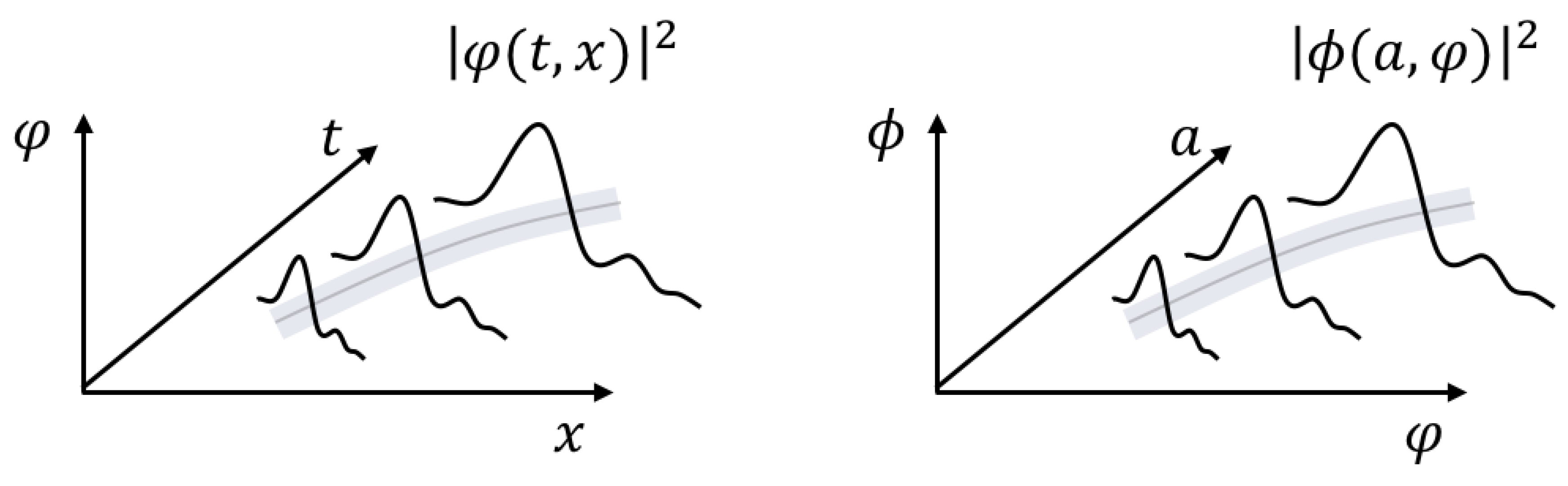
8
Eventually, these inhomogeneous modes are interpreted as particles and gravitons propagating in the homogeneous and isotropic background spacetime.
9
Spinorial and vector fields can be considered as well.
10
For convenience, the scalar field has been rescaled according to φ 2 φ .
11
Unless otherwise indicated, we always consider cosmic time, i.e., N = 1 .
12
Recall that the scalar field φ has been rescaled according to φ 2 φ , see f.n. 10.
13
This is the basis of the reasoning made in [41]. The trajectory followed by a test particle can be seen either as a geodesic in a given metric or as a non-geodesic in a conformal metric under the action of some potential [41] (see also Refs. [42,43]).
14
Let us bear in mind, however, that it is only an analogy.
15
This way of obtaining the Klein–Gordon equation from the Hamiltonian constraint of a test particle that propagates in the spacetime has been well-known for a long time. It can be seen, for instance, in Ref. [44]. However, it is not customarily used in quantum field theory.
16
The exact meaning of “sufficiently localised” is specified in Section 5.
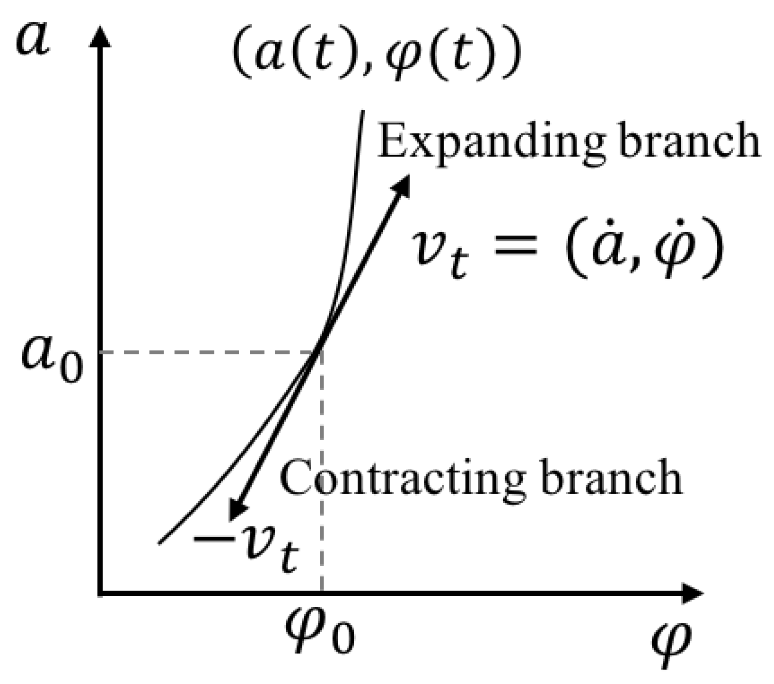
17
By a future directed vector in the minisuperspace, we mean a vector positively oriented with respect to the scale factor component, which is the time-like variable of the minisuperspace.
18
We do not call it second quantisation of the universe because in this formalism the field ϕ can represent many universes.
19
This can explicitly be seen in a very simplified cosmological model [38]. As we show below, it might have consequences in the quantum creation of universes.
20
In the quantisation of a complex scalar field, it would be full of particle–antiparticle pairs.
21
From now on, we omit the hats on top of the operators to ease the notation.
22
Recall that the field φ was rescaled according to φ 2 φ , see f.n. 10.
23
The Euclidean gap also prevent matter and antimatter from collapse
24
Classically, the changes, g ˜ μ ν = Δ 1 g μ ν and d λ = m Δ 1 d τ , transform the action in Equation (21) [41] into
S = d λ 1 2 h ˜ i j d x i d λ d x j d λ V ( r ) ,
which, far from the even horizon, corresponds to the action of a test particle moving in a flat space under the action of the Newtonian potential, V ( x ) = M r (in units, G = c = 1 ). It means that the trajectory of a free test particle in a Schwarzschild spacetime is equivalent, far from the event horizon, to the trajectory of the test particle in a flat space under the action of the Newtonian potential, as it is expected. Similarly, the Schrödinger equation (Equation (92)) is the non-relativistic version of the corresponding Klein–Gordon equation (Equation (36)).
25
For instance, in the case of a flat DeSitter spacetime, the modes with physical wavelengths λ p h y s much smaller than the cosmological horizon, L h = 1 H 0 , can be interpreted in terms of particles with highly definite trajectories [41].
26
This will be done elsewhere.
Figure 1. Foliation of the spacetime into space and time. (Left) In flat spacetime, the lines of constant x i are orthogonal to the spatial hypersurfaces Σ t and the coordinate time t coincides with the proper time, τ . (Right) In a curved spacetime, there is a shift, given by N i d t , between the point that would have been reached if the particle would have followed the orthonormal vector of the hypersurface, n μ at x i in Σ t , and the actual point of coordinates x i in d Σ t + d t . The proper time τ is now “lapsed” with respect to the coordinate time, t.
Galaxies 07 00050 g001
Figure 2. The evolution of the universe can be seen as a parameterised trajectory in the minisuperspace. Trajectories in the minisuperspace with positive zero components of the tangent vector entail a growing value of the scale factor so they represent expanding universes. Analogously, those with negative zero component in the tangent vector describe contracting universes.
Galaxies 07 00050 g002
Figure 3. (Left) In a quantum field theory, the field is described in terms of particles that follow with the highest probability the classical trajectories given by the geodesics with however some uncertainties in their positions. (Right) The wave function that describes the quantum state of the spacetime and the matter fields, all together, can be seen as a another field, say a super-field, that propagates in the minisuperspace. The universes can then be seen as “test” particles following classical trajectories in the minisuperspace with quantum uncertainties given by the Schrödinger equation of their matter fields.
Galaxies 07 00050 g003
Figure 4. The creation of universes in entangled pairs [49]. To obtain the correct value of the Schrödinger equation in the two universes, their physical time variables must be reversely related. In that case, particles moving in the symmetric universe look as though they were moving backward in time so they are naturally identified with the antiparticles that are left in the observer’s universe. The primordial matter–antimatter asymmetry observed in the context of a single universe would thus be restored in the multiverse. Particles and antiparticles do not collapse at the onset because the Euclidean gap that exists between the two newborn universes [49,57].
Galaxies 07 00050 g004

