Faraday Tomography Tutorial


Abstract
1. Introduction
2. Basics of Faraday Tomography
2.1. Faraday Tomography
2.2. RM Synthesis
2.3. RM CLEAN
RM Ambiguity
2.4. QU-Fitting with MCMC
2.5. Comparison of Methods
3. Tutorial
3.1. Data
3.2. Scripts
3.3. Practical Exercises
3.3.1. RM Synthesis
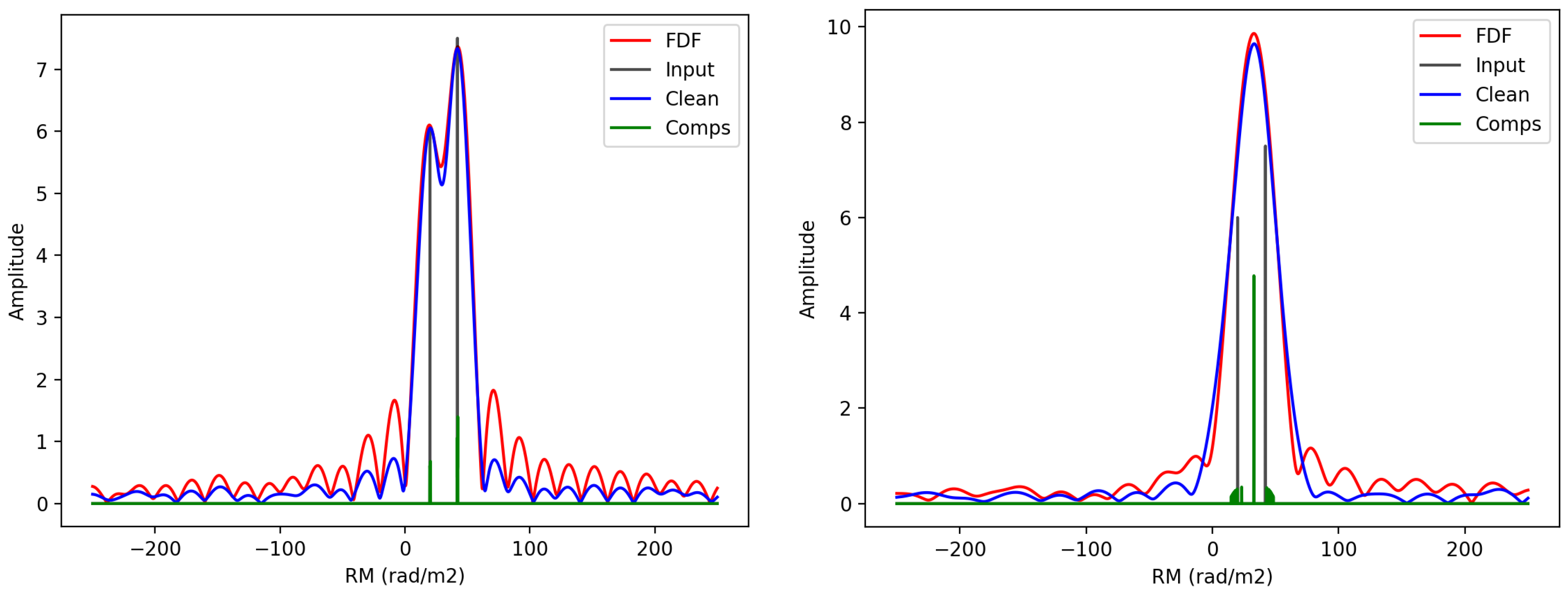
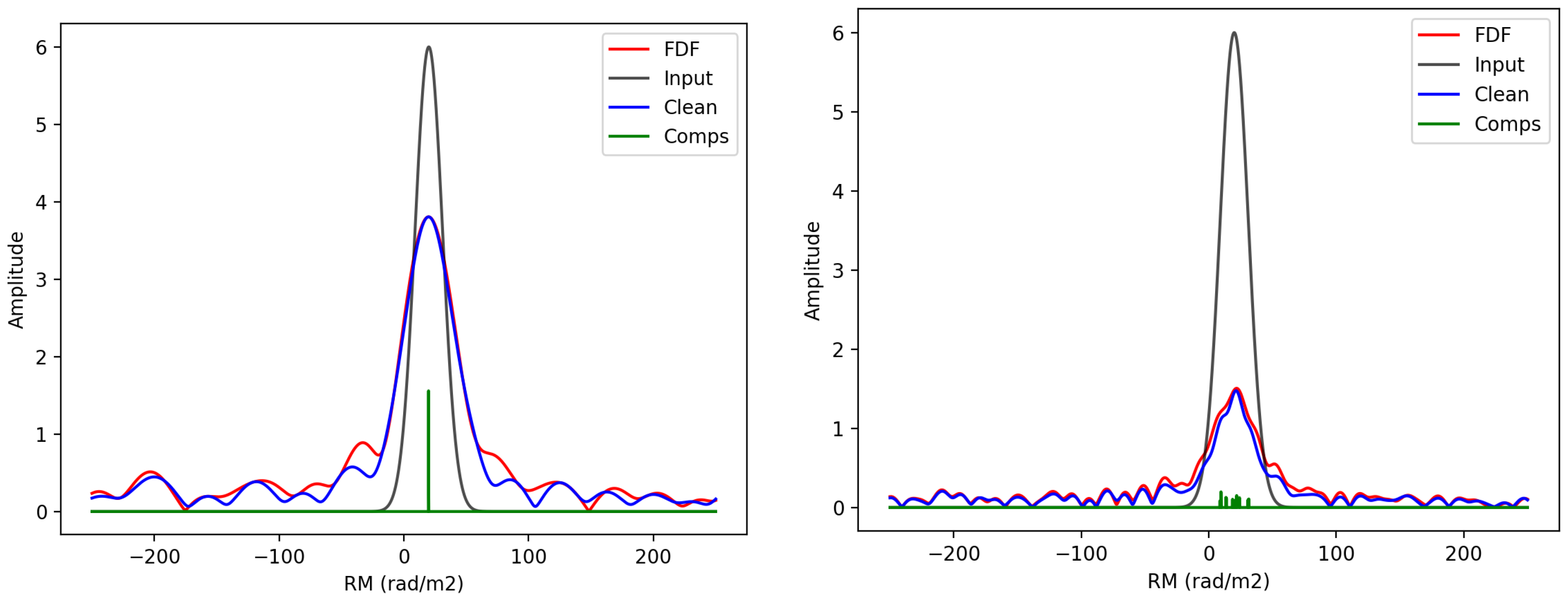
3.3.2. RM CLEAN
3.3.3. QU-Fitting with MCMC
4. Summary
Author Contributions
Funding
Acknowledgments
Conflicts of Interest
References
- Van Haarlem, M.P.; Wise, M.W.; Gunst, A.W.; Heald, G.; McKean, J.P.; Hessels, J.W.T.; de Bruyn, A.G.; Nijboer, R.; Swinbank, J.; Fallows, R.; et al. LOFAR: The LOw-Frequency ARray. Astron. Astrophys. 2013, 556, A2. [Google Scholar] [CrossRef]
- Tingay, S.J.; Goeke, R.; Bowman, J.D.; Emrich, D.; Ord, S.M.; Mitchell, D.A.; Morales, M.F.; Booler, T.; Crosse, B.; Wayth, R.B.; et al. The Murchison Widefield Array: The Square Kilometre Array Precursor at Low Radio Frequencies. Publ. Astron. Soc. Aust. 2013, 30, e007. [Google Scholar] [CrossRef]
- McConnell, D.; Allison, J.R.; Bannister, K.; Bell, M.E.; Bignall, H.E.; Chippendale, A.P.; Edwards, P.G.; Harvey-Smith, L.; Hegarty, S.; Heywood, I.; et al. The Australian Square Kilometre Array Pathfinder: Performance of the Boolardy Engineering Test Array. Publ. Astron. Soc. Aust. 2016, 33, e042. [Google Scholar] [CrossRef]
- Jonas, J.; MeerKAT Team. The MeerKAT Radio Telescope. In Proceedings of the MeerKAT Science: On the Pathway to the SKA (MeerKAT2016), Stellenbosch, South Africa, 25–27 May 2016; p. 1. [Google Scholar]
- Brentjens, M.A. Wide field polarimetry around the Perseus cluster at 350 MHz. Astron. Astrophys. 2011, 526, A9. [Google Scholar] [CrossRef]
- Jelić, V.; de Bruyn, A.G.; Pandey, V.N.; Mevius, M.; Haverkorn, M.; Brentjens, M.A.; Koopmans, L.V.E.; Zaroubi, S.; Abdalla, F.B.; Asad, K.M.B.; et al. Linear polarization structures in LOFAR observations of the interstellar medium in the 3C 196 field. Astron. Astrophys. 2015, 583, A137. [Google Scholar] [CrossRef]
- Burn, B.J. On the depolarization of discrete radio sources by Faraday dispersion. Mon. Not. R. Astron. Soc. 1966, 133, 67–83. [Google Scholar] [CrossRef]
- Brentjens, M.A.; de Bruyn, A.G. Faraday rotation measure synthesis. Astron. Astrophys. 2005, 441, 1217–1228. [Google Scholar] [CrossRef]
- Brentjens, M.A. Radio Polarimetry in 2.5D. Ph.D. Thesis, University of Groningen, Groningen, The Netherlands, 2007. [Google Scholar]
- Heald, G.; Braun, R.; Edmonds, R. The Westerbork SINGS survey. II Polarization, Faraday rotation, and magnetic fields. Astron. Astrophys. 2009, 503, 409–435. [Google Scholar] [CrossRef]
- Heald, G. The Faraday rotation measure synthesis technique. Cosm. Magn. Fields 2009, 259, 591–602. [Google Scholar] [CrossRef]
- Farnsworth, D.; Rudnick, L.; Brown, S. Integrated Polarization of Sources at λ∼ 1 m and New Rotation Measure Ambiguities. Astron. J. 2011, 141, 191. [Google Scholar] [CrossRef]
- O’Sullivan, S.P.; Brown, S.; Robishaw, T.; Schnitzeler, D.H.F.M.; McClure-Griffiths, N.M.; Feain, I.J.; Taylor, A.R.; Gaensler, B.M.; Landecker, T.L.; Harvey-Smith, L.; et al. Complex Faraday depth structure of active galactic nuclei as revealed by broad-band radio polarimetry. Mon. Not. R. Astron. Soc. 2012, 421, 3300–3315. [Google Scholar] [CrossRef]
- Sun, X.H.; Rudnick, L.; Akahori, T.; Anderson, C.S.; Bell, M.R.; Bray, J.D.; Farnes, J.S.; Ideguchi, S.; Kumazaki, K.; O’Brien, T.; et al. Comparison of Algorithms for Determination of Rotation Measure and Faraday Structure. I. 1100–1400 MHz. Astron. J. 2015, 149, 60. [Google Scholar] [CrossRef]
- Bell, M.R.; Enßlin, T.A. Faraday synthesis. The synergy of aperture and rotation measure synthesis. Astron. Astrophys. 2012, 540, A80. [Google Scholar] [CrossRef]
- Sridhar, S.S.; Heald, G.; van der Hulst, J.M. cuFFS: A GPU-accelerated code for Fast Faraday rotation measure Synthesis. Astron. Comput. 2018, 25, 205–212. [Google Scholar] [CrossRef]
- Walt, S.V.D.; Colbert, S.C.; Varoquaux, G. The NumPy Array: A Structure for Efficient Numerical Computation. Comput. Sci. Eng. 2011, 13, 22–30. [Google Scholar] [CrossRef]
- Hunter, J.D. Matplotlib: A 2D graphics environment. Comput. Sci. Eng. 2007, 9, 90–95. [Google Scholar] [CrossRef]
- Kluyver, T.; Ragan-Kelley, B.; Pérez, F.; Granger, B.; Bussonnier, M.; Frederic, J.; Kelley, K.; Hamrick, J.; Grout, J.; Corlay, S.; et al. Jupyter Notebooks—A publishing format for reproducible computational workflows. In Positioning and Power in Academic Publishing: Players, Agents and Agendas; Loizides, F., Schmidt, B., Eds.; IOS Press: Amsterdam, The Netherlands, 2016; pp. 87–90. [Google Scholar]
| 1. | |
| 2. | |
| 3. |


| RM Synthesis + RM CLEAN | QU-fitting | |
|---|---|---|
| Model assumption | ◯ Not explicitly necessary | × Needed |
| Estimation of | ⨂ Not bad | ◯ Good (If appropriate models are given) |
| Estimation of error | × Impossible | ◯ Possible |
| Computational cost | ◯ Cheap | × Expensive |
| Amp. [arb. units] | [deg.] | |||
|---|---|---|---|---|
| 20 | 6 | 30 | - | |
| 20 | 6 | 30 | - | |
| 42 | 7.5 | −60 | - | |
| 20 | 6 | 30 | 11 | |
| 20 | 6 | 30 | 22 | |
| 20 | 6 | 30 | 44 | |
| 20 | 6 | 30 | 22 | |
| 42 | 7.5 | −60 | 11 |
© 2018 by the authors. Licensee MDPI, Basel, Switzerland. This article is an open access article distributed under the terms and conditions of the Creative Commons Attribution (CC BY) license (http://creativecommons.org/licenses/by/4.0/).
Share and Cite
Ideguchi, S.; Miyashita, Y.; Heald, G. Faraday Tomography Tutorial. Galaxies 2018, 6, 140. https://doi.org/10.3390/galaxies6040140
Ideguchi S, Miyashita Y, Heald G. Faraday Tomography Tutorial. Galaxies. 2018; 6(4):140. https://doi.org/10.3390/galaxies6040140
Chicago/Turabian StyleIdeguchi, Shinsuke, Yoshimitsu Miyashita, and George Heald. 2018. "Faraday Tomography Tutorial" Galaxies 6, no. 4: 140. https://doi.org/10.3390/galaxies6040140
APA StyleIdeguchi, S., Miyashita, Y., & Heald, G. (2018). Faraday Tomography Tutorial. Galaxies, 6(4), 140. https://doi.org/10.3390/galaxies6040140