Better Galactic Mass Models through Chemistry

Abstract

With the upcoming release of the Gaia catalog and the many multiplexed spectroscopic surveys on the horizon, we are rapidly moving into a new data-driven era in the study of the Milky Way’s stellar halo. When combined, these data sets will give us a many-dimensional view of stars in accreted structures in the halo that includes both dynamical information about their orbits and chemical information about their formation histories. Using simulated data from the state-of-the-art Latte simulations of Milky-Way-like galaxies, which include hydrodynamics, feedback, and chemical evolution in a cosmological setting, we demonstrate that while dynamical information alone can be used to constrain models of the Galactic mass distribution in the halo, including the extra dimensions provided by chemical abundances can improve these constraints as well as assist in untangling different accreted components.

1. Introduction

Our knowledge of the Galaxy in which we live, the Milky Way (MW), is poised to undergo a revolution in the next ten years thanks to a new generation of state-of-the-art stellar surveys. These include photometric surveys like PanSTARRS [1] and LSST [2], spectroscopic surveys like 4MOST [3], DESI [4], WEAVE [5], and Subaru-PFS [6], and astrometric surveys starting with Gaia [7] and extending to LSST and WFIRST [8]. The Galactic renaissance will also include far greater insight into the chemical abundances of stars thanks to efforts like the Cannon [9], which can translate the abundance patterns generated from smaller high-resolution spectroscopic surveys like APOGEE [10], GALAH [11], and the Gaia-ESO survey [12] into the larger medium- and low-resolution spectroscopic surveys listed above. It is not an exaggeration to say that ten years from now we can expect to have complete phase-space information for stars in the Galaxy nearly to its virial radius, complemented by 10–20 dimensions of chemical abundance information. This new high-dimensional view of the Galaxy demands new approaches to understanding its contents. Here we discuss how this combined phase and abundance space will be uniquely powerful for setting constraints on the MW’s dark matter (DM) distribution and untangling the building blocks of its accreted stellar halo, allowing us to use our Galaxy as a time machine to study ancient dwarf galaxies.

Currently our knowledge of the distribution of stars in the MW is limited to the region within about 120 kpc [13], less than half of what we imagine to be the full extent of its dark halo. Because of this limited information, our knowledge of the shape and mass of the MW’s DM halo is equally limited: measurements of its total mass disagree by a factor of ~4 [14] and our understanding of its shape and radial profile is still poorly constrained enough to be controversial [15,16] especially in light of new estimates of the mass of its largest companion, the Large Magellanic Cloud [17,18]. This makes it difficult to place our Galaxy in a cosmological context in order to use it as a test of DM theories, since many predictions from cosmological simulations scale with mass and concentration [19].

2. Methods

Stars in the accreted stellar halo of the Milky Way provide one of the few sources of information about the outer extents of the Galactic dark halo. Most of these stars are part of structures called tidal streams (e.g., [20]) created by the disruption of ancient dwarf satellite galaxies of the MW, and are expected to reach to the MW’s virial radius and beyond [21,22]. Since the stars in tidal streams all have similar orbits, tidal streams are, in principle, more sensitive to the radial profile and shape of the halo than the orbits of individual bound dwarf galaxies or globular clusters, and so are valuable for constraining the MW’s shape and mass. Furthermore the approximately isotropic nature of accretion (although see [23]) samples orbits well out of the plane of the Galactic disk and at much larger distances, giving us a more complete map of the gravitational forces exerted by our Galaxy than we could otherwise achieve.

2.1. The Action Space of Stellar Orbits

One approach to mapping the Milky Way’s dark halo with tidal streams is to work in the space of their actions $\mathbf{J}$, which are defined for stars on bound orbits in a system described by a Hamiltonian $\mathcal{H}$ as a canonical transformation of their positions $\mathbf{x}$ and momenta $\mathbf{p}$, such that for each component $x_i$,

$$J_i=\oint p_{i}d{x}_i,$$

(1)

where the integral is over one cycle of the coordinate $x_i$. When defined in this way, a star’s actions $\mathbf{J}$ are adiabatic invariants (i.e., integrals of the motion) and the angles $\theta$ evolve linearly in time with frequencies $\mathrm{\Omega }$:

$$\begin{array}{ccc}\hfill {\theta }_i& =& {\mathrm{\Omega }}_{i}t+{\theta }_{i,0},\hfill \end{array}$$

(2)

$$\begin{array}{ccc}\hfill {\mathrm{\Omega }}_i& =& \frac{\mathsf{\partial }\mathcal{H}}{\mathsf{\partial }{J}_i}.\hfill \end{array}$$

(3)

For more background on action-angle variables we refer the reader to the discussions in Chapter 3 of [24] or Chapter 10 of [25]; for more detailed information on the techniques described in this section see [26,27].

For a tidal stream, in which all the stars began life within the small (compared to the MW) phase-space volume of a dwarf galaxy, their actions are persistently similar unless the host galaxy (in this case the MW) undergoes a major merger that non-adiabatically transforms the gravitational potential. The actions thus conveniently label stars in each tidal stream by their orbit family, and the small cluster in $\mathbf{J}$ representing the stream can be treated using linear transformations [28]. Furthermore, a stellar halo made of accreted small galaxies, as predicted by theories of cold DM, will exhibit a high degree of clustering in the space of its actions even for structures that are spread across the Galaxy (Figure 1, panels A and B). This space is thus ideal for separating different accreted structures from one another [29,30,31].

Studying tidal streams in action space requires assuming a global gravitational potential, but the structure of action space itself gives insight into the correct potential to use. As shown by comparing panels B and C of Figure 1, only when the assumed potential is a close representation of the true mass distribution will the action space of the stellar demonstrate the expected degree of clustering [26,33,34]. A statistical measure of the degree of clustering can thus be used as the figure of merit to determine the best-fit potential [26,27,35]. We will describe the quantification of clustering in Section 2.2. The advantage of this method of determining the Galactic gravitational potential, especially in the context of the many upcoming stellar surveys, is twofold. First, it does not require that individual streams are identified or stars assigned to membership in a particular stream, merely that the stars in the fitting sample come mainly from the accreted stellar halo so that the assumption of an intrinsically clustered distribution is satisfied. Second, the method is agnostic as to which labels are used as dimensions, so long as the stars in each stream demonstrate some correlation with each other in those labels and at least some of them depend on the gravitational potential. This means that if chemical abundance information is also available for the stars in the fitting sample, these labels can be added as extra dimensions. The chemical abundances of stars from a given progenitor galaxy should be correlated through their shared star formation history, so this extra information should improve the ability to constrain the gravitational potential by, for example, differentiating stars from progenitors with different masses that accreted on similar orbits.

2.2. Measuring Clustering in Actions

To quantify the degree of clustering in the distribution of actions $\mathbf{J}$ and abundances $\mathbf{Z}$, given a guess for the gravitational potential $\mathsf{\Phi }$, we use the mutual information (MI) statistic [36], defined as the relative entropy between the target distribution $p_{\mathsf{\Phi }}(\mathbf{J},\mathbf{Z})$ and a “shuffled” version ${\tilde{p}}_{\mathsf{\Phi }}(\mathbf{J},\mathbf{Z})$:

$$MI\left(\mathsf{\Phi }\right)\equiv \int p_{\mathsf{\Phi }}(\mathbf{J},\mathbf{Z})ln\frac{p_{\mathsf{\Phi }}(\mathbf{J},\mathbf{Z})}{{\tilde{p}}_{\mathsf{\Phi }}(\mathbf{J},\mathbf{Z})}d\mathbf{J}d\mathbf{Z}$$

(4)

The distribution ${\tilde{p}}_{\mathsf{\Phi }}$ is constructed by randomizing the $\mathbf{J}$ and $\mathbf{Z}$ coordinates of each star relative to one another. This transformation preserves the one-dimensional marginal distributions along each coordinate, and is equivalent to the product of the marginals:

$${\tilde{p}}_{\mathsf{\Phi }}(\mathbf{J},\mathbf{Z})=\prod _i{p}_{\mathsf{\Phi }}\left(J_i\right|J_{\ne i},\mathbf{Z})\prod _j{p}_{\mathsf{\Phi }}\left(Z_j\right|Z_{\ne j},\mathbf{J}).$$

(5)

To calculate the MI for a given set of stars, we first calculate the stellar actions assuming the potential $\mathsf{\Phi }$ and use the density estimation code EnLink [37] to calculate the densities $p_{\mathsf{\Phi }}$ and ${\tilde{p}}_{\mathsf{\Phi }}$ in $(\mathbf{J},\mathbf{Z})$ space at the location of each star. We then use Monte Carlo integration to estimate the MI by summation over all stars in the sample:

$$MI\left(\mathsf{\Phi }\right)=\sum _{i=1}^{N_{*}}ln\frac{p_{i,\mathsf{\Phi }}(\mathbf{J},\mathbf{Z})}{{\tilde{p}}_{i,\mathsf{\Phi }}(\mathbf{J},\mathbf{Z})}$$

(6)

As shown in Figure 2, the more clustered the distribution is, the greater the difference with the product of its marginals, and hence the larger the value of $MI\left(\mathsf{\Phi }\right)$. The maximum value of $MI\left(\mathsf{\Phi }\right)$ identifies the most clustered distribution and hence the best-fit gravitational potential.

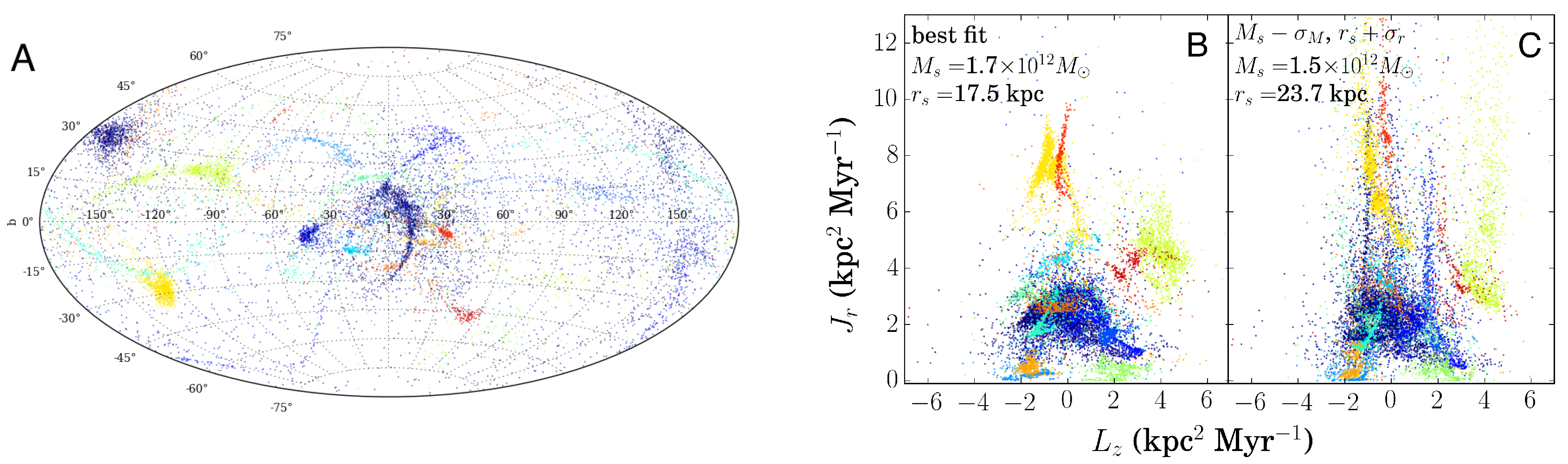
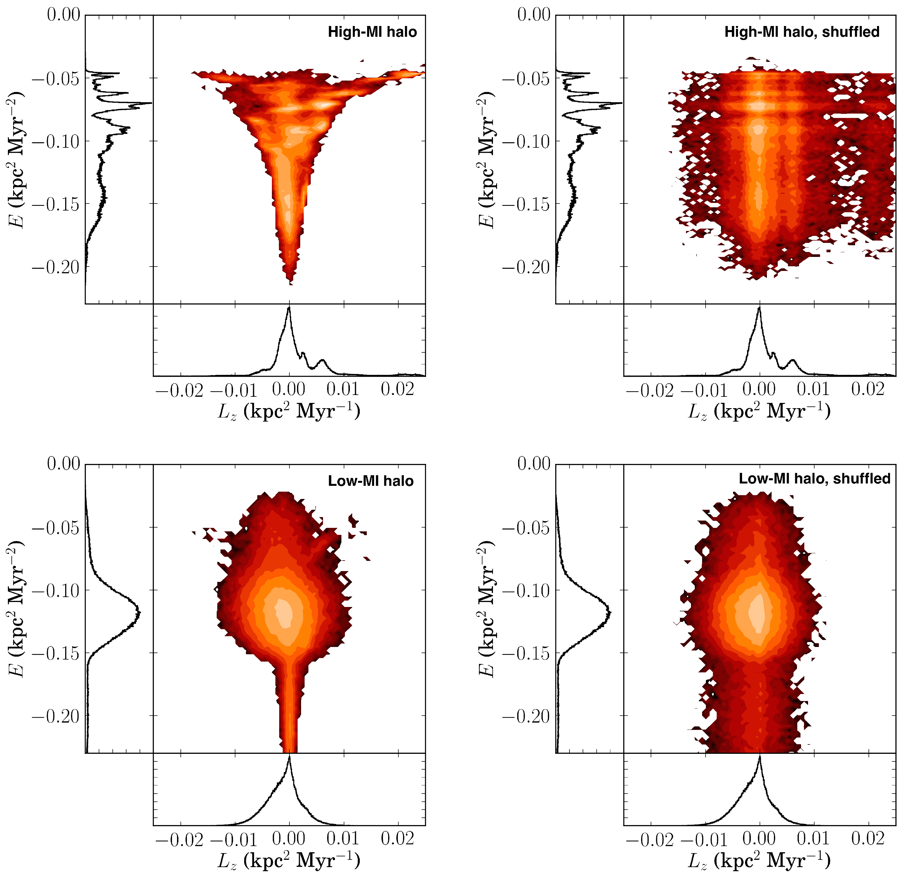
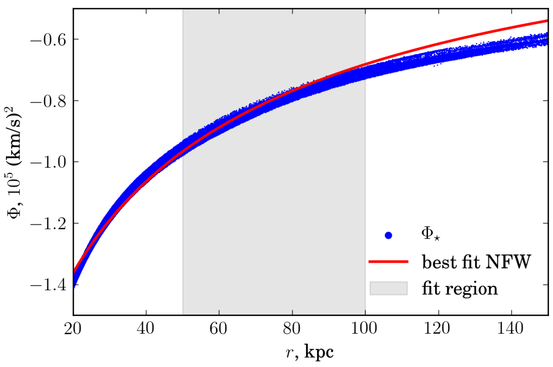
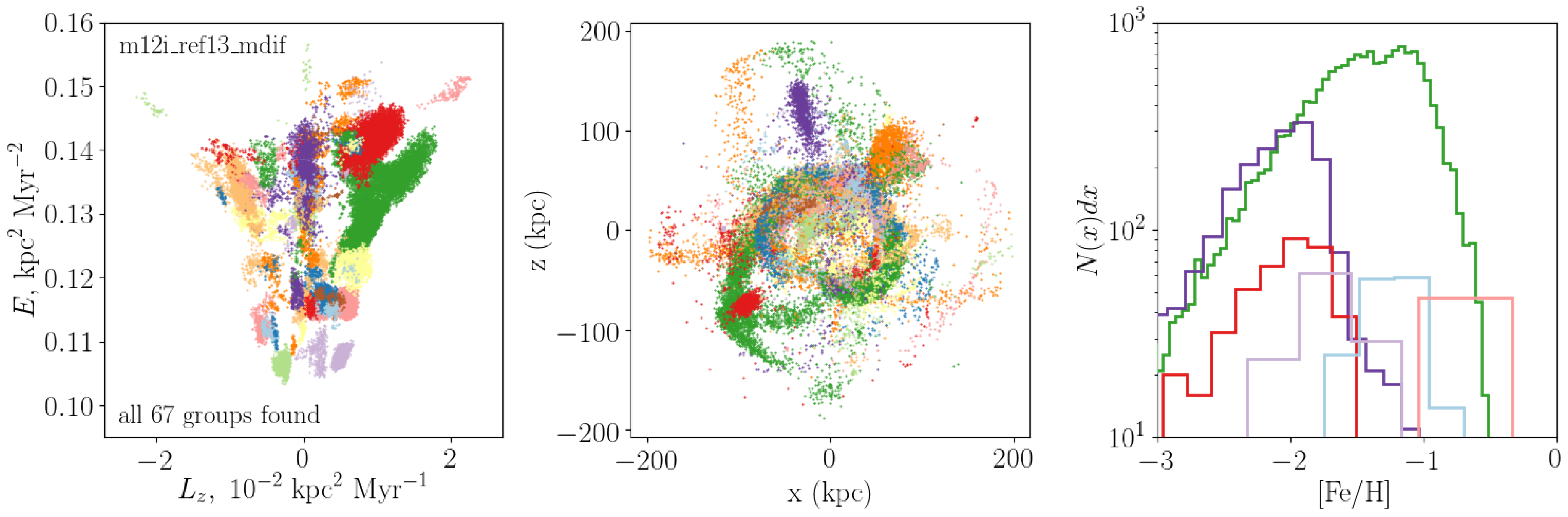
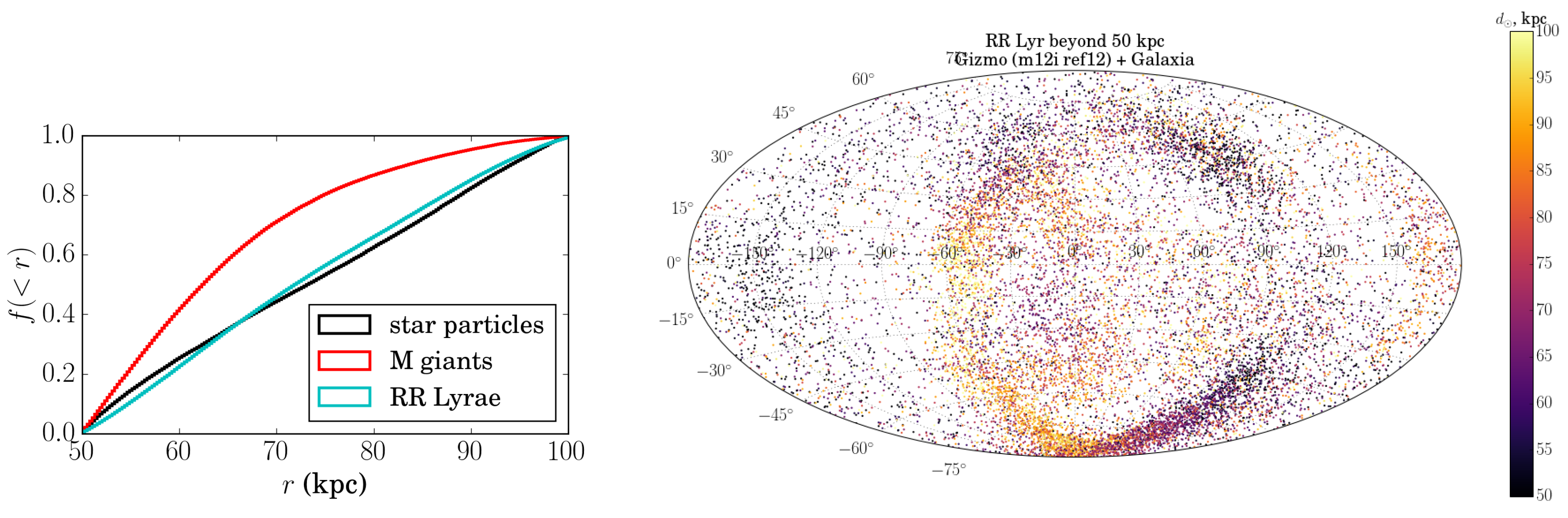
2.3. Simulating the Accreted Stellar Halo

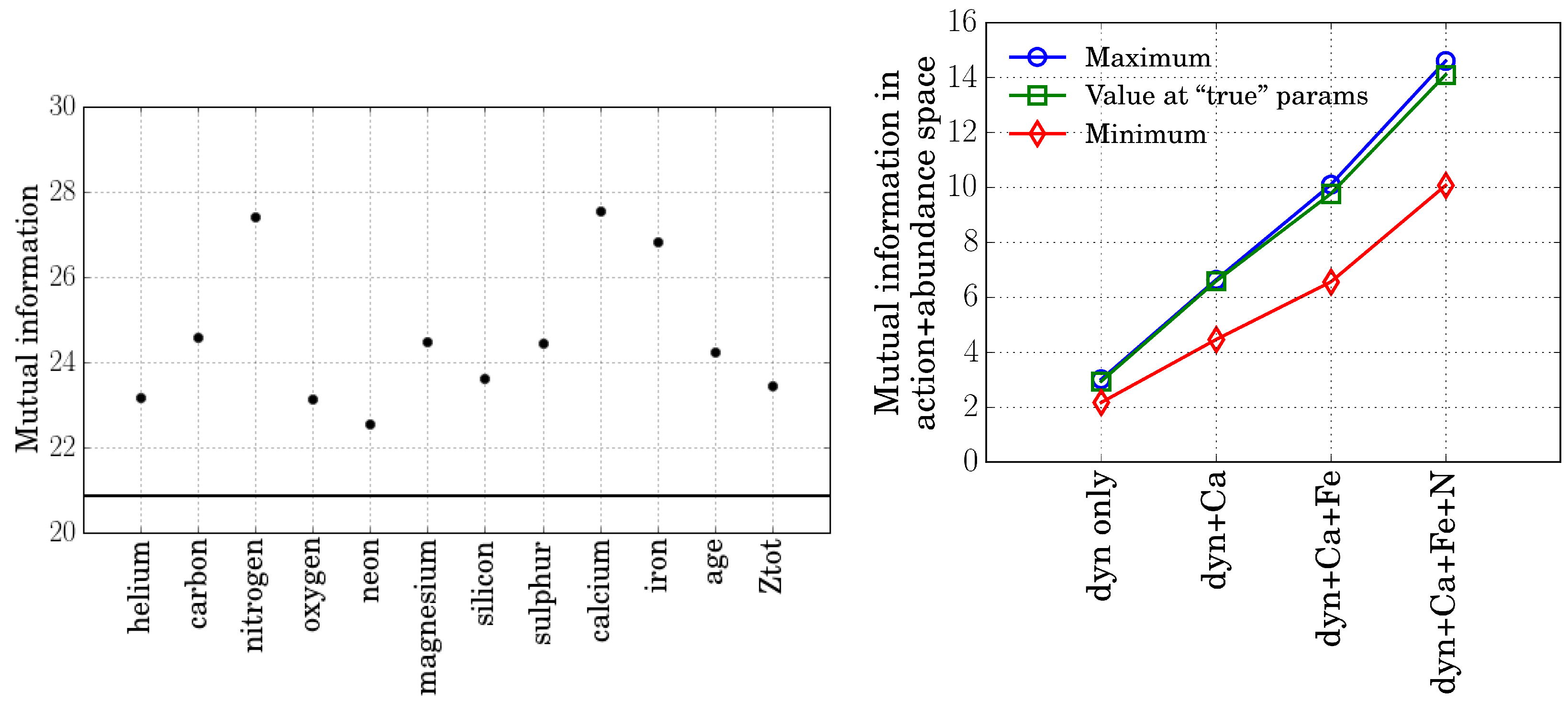
To test the hypothesis that adding chemical abundance information can improve constraints on the Galactic gravitational potential, we used the simulated galaxy m12i from the Latte simulation suite, described in [38]. This MW-like simulated galaxy is the product of a high-resolution, cosmological zoom-in simulation that uses the FIRE-2 feedback recipe [39] to follow star formation and the evolution of stellar populations. The simulation tracks the evolution of ten chemical elements produced by supernovae (types I and II) and winds from evolved stars. For the examples shown here we used the second-highest resolution version of the simulation, in which star particles have $m_p$~56,500 M${}_{\odot }$. For this preliminary test, we selected star particles in a region between 50 and 100 kpc from the main galaxy’s center to avoid the galactic stellar and gas disk.

Using this selection as the fitting sample, we modeled the galactic mass distribution with a spherical Navarro-Frenk-White form [40] with scale radius $r_s$ and scale density ${\rho }_s$, parameterized in terms of the enclosed mass $M_s$ at the scale radius,

$$M_s\equiv M_{encl}\left(r_s\right)=4\pi {\rho }_s{r}_s^3\left(ln2-\frac{1}{2}\right),$$

(7)

In terms of $M_s$ and $r_s$, the potential is

$$\mathsf{\Phi }\left(r\right)=-G\frac{M_s}{ln2-1/2}\frac{ln(1+r/r_s)}{r}$$

(8)

where G is Newton’s constant. The choice of $M_s$ over ${\rho }_s$ as the mass parameter is motivated by the sensitivity of stellar orbits to the enclosed mass rather than the local density, and avoids severe degeneracies between parameters during the fit. This functional form ignores the triaxiality of the halo but can adequately approximate the radial profile of the gravitational potential over a limited radial range. To check the results of the fit using the halo sample, we also fit the same functional form directly to the gravitational potentials of the stars as calculated directly by the simulation (Figure 3).

3. Results

Calculating the MI for a distribution involves estimating the density from a finite number of points, so adding extra dimensions is costly and can introduce noise in the MI value and hence in the best fit. So before adding all ten chemical abundances tracked by the simulation, we first looked at the change in the MI when adding each abundance separately to the actions, while assuming the potential fit directly to the values calculated from the simulation and shown in Figure 3. A larger increase in MI when a given abundance is added signals a larger degree of clustering in that dimension and should correspond to more additional constraining power on the potential when added to the actions. The left panel of Figure 4 shows that indeed some abundances appear to contain more extra information than others, probably as a result of the assumptions about how different elements are produced in the simulation. Guided by this result we selected nitrogen, calcium, and iron to use as additional labels in fitting the gravitational potential. We caution that the result that these three abundances were most informative should not be over-interpreted, given the simplified yield tables used in the simulations; this is more a proof of concept and a demonstration of a technique that could be used on future data sets.

Next we carried out a fit of the gravitational potential by varying the parameters $M_s$ and $r_s$ of the model over an iteratively refined grid in parameter space, first using only the actions and then adding the extra chemical abundance dimensions one at a time. We then looked at the contrast between the maximum value of the MI (at the best-fit potential) and the value far from the best-fit peak, and likewise at the value of the MI for the parameters obtained when the NFW function was fit to the potential values calculated directly from the simulation (i.e., Figure 3). We compare to this baseline MI far from the best fit because the MI is an entropy and therefore an extensive quantity, meaning that its absolute value will increase somewhat when a dimension is added even if that dimension is not informative. However, as is evident from the right panel of Figure 4, the difference between the peak and baseline MI values increases as new abundance dimensions are introduced, suggesting that the height of the best-fit peak is increasing (and therefore the confidence interval around the best fit should shrink).

Once the best-fit potential is obtained, the different building blocks of the accreted stellar halo can be separated from one another by running a group-finding algorithm on the same space of actions and abundances. Here again one expects that adding abundance information to constants-of-motion space can help distinguish the different components. Figure 5 illustrates how groups found in constants of motion space alone using EnLink (left) indeed represent different tidal streams (center) but also have distinct, though overlapping, abundance distributions (right). This bodes well for future attempts to reconstruct the component dwarf galaxies of the Milky Way’s stellar halo.

4. Discussion

These results, obtained using the star particle data from a realistic simulation of a MW-like galaxy, indicate that studying tidal streams in the combined space of orbits and abundances is a promising direction both for constraining the Galactic gravitational potential and reconstructing the destroyed galaxies of the halo. Most interestingly, these results were obtained with a simulation in which the diffusion of chemical elements into star-forming gas was not implemented, which produces broader abundance distributions compared to those shown in Figure 5, and broader than the known abundance distributions of bound MW dwarf galaxies (Escala et al., in prep). Thus these results can be understood as a conservative estimate for the extra information contributed by elemental abundances.

On the other hand, these results assumed perfect data without observational uncertainties; furthermore, those uncertainties depend strongly on the type of stellar tracer for both phase-space coordinates and abundances. For example, variable-star standard candles like RR Lyra stars will have extremely precise distances [13,41] but pose difficulties when obtaining precise radial velocities or elemental abundances thanks to the same physics that makes them standard candles. Conversely, bright, cool giant stars will be visible to great distances and have well-constrained abundances and RVs, but less precise distances. Even more fundamentally, different stellar tracers have different specific frequencies depending on the underlying metal content of the population; for example, RR Lyr are more common in metal-poor populations and M giants are more common in metal-rich populations. As a result, they probe different regions of the Galaxy, and different regions in the stellar halo in particular, as illustrated in the left panel of Figure 6.

To better account for both the variety of stellar tracers and the range of expected observational errors, we are now updating the synthetic survey code Galaxia [42] to self-consistently resample the high-resolution Latte simulations with synthetic stars drawn from PARSEC isochrones [43]. A preliminary example is shown in the right panel of Figure 6. When complete, this machinery will allow us to make robust, detailed comparisons between the Milky Way and simulated galaxies, and accurately forecast the performance of various methods to constrain the Galactic gravitational potential and untangle the accretion history of the stellar halo.

References

1. Chambers, K.C.; Magnier, E.A.; Metcalfe, N.; Flewelling, H.A.; Huber, M.E.; Waters, C.Z.; Denneau, L.; Draper, P.W.; Farrow, D.; Finkbeiner, D.P.; et al. The Pan-STARRS1 Surveys. arXiv 2016, arXiv:astro-ph.IM/1612.05560. [Google Scholar]
2. LSST Science Collaboration; Abell, P.A.; Allison, J.; Anderson, S.F.; Andrew, J.R.; Angel, J.R.P.; Armus, L.; Arnett, D.; Asztalos, S.J.; Axelrod, T.S.; et al. LSST Science Book, Version 2.0. arXiv 2009, arXiv:astro-ph.IM/0912.0201. [Google Scholar]
3. De Jong, R.S.; Bellido-Tirado, O.; Chiappini, C.; Depagne, É.; Haynes, R.; Johl, D.; Schnurr, O.; Schwope, A.; Walcher, J.; Dionies, F.; et al. 4MOST: 4-Metre Multi-Object Spectroscopic Telescope. In Proceedings of the SPIE Astronomical Instrumentation and Telescopes Conference, Amsterdam, The Netherlands, 1–6 July 2012; McLean, I.S., Ramsay, S.K., Takami, H., Eds.; SPIE: Bellingham, DC, USA, 2012; Volume 8446. [Google Scholar]
4. Flaugher, B.; Bebek, C. The Dark Energy Spectroscopic Instrument (DESI). In Proceedings of the Ground-based and Airborne Instrumentation for Astronomy V, Montréal, QC, Canada, 22 June 2014; Ramsay, S.K., McLean, I.S., Takami, H., Eds.; SPIE: Bellingham, DC, USA, 2014; Volume 9147. [Google Scholar]
5. Dalton, G.; Trager, S.C.; Abrams, D.C.; Carter, D.; Bonifacio, P.; Aguerri, J.A.L.; MacIntosh, M.; Evans, C.; Lewis, I.; Navarro, R.; et al. WEAVE: The next generation wide-field spectroscopy facility for the William Herschel Telescope. In Proceedings of the Ground-based and Airborne Instrumentation for Astronomy IV, Amsterdam, The Netherlands, 1 July 2012; Ramsay, S.K., Takami, H., Eds.; SPIE: Bellingham, DC, USA, 2012; Volume 8446. [Google Scholar]
6. Chiba, M.; Cohen, J.; Wyse, R.F.G. Galactic Archaeology with the Subaru Prime Focus Spectrograph. In Proceedings of the International Astronomical Union, Honolulu, HI, USA, 3 August 2015; Bragaglia, A., Arnaboldi, M., Rejkuba, M., Romano, D., Eds.; IAU: Paris, France, 2016; Volume 317, pp. 280–281. [Google Scholar]
7. Gaia Collaboration; Prusti, T.; de Bruijne, J.H.J.; Brown, A.G.A.; Vallenari, A.; Babusiaux, C.; Bailer-Jones, C.A.L.; Bastian, U.; Biermann, M.; Evans, D.W.; et al. The Gaia mission. Astron. Astrophys. 2016, 595, A1. [Google Scholar]
8. Spergel, D.; Gehrels, D.; Baltay, C.; Bennett, D.; Breckinridge, J.; Donahue, M.; Dressler, A.; Gaudi, B.S.; Greene, T.; Guyon, O.; et al. Wide-Field InfrarRed Survey Telescope-Astrophysics Focused Telescope Assets WFIRST-AFTA 2015 Report. arXiv 2015, arXiv:1503.03757. [Google Scholar]
9. Ness, M.; Hogg, D.W.; Rix, H.W.; Ho, A.Y.Q.; Zasowski, G. The Cannon: A data-driven approach to Stellar Label Determination. Astrophys. J. Suppl. Ser. 2015, 808, 21. [Google Scholar] [CrossRef]
10. Alam, S.; Albareti, F.D.; Prieto, C.A.; Anders, F.; Anderson, S.F.; Andrews, B.H.; Armengaud, E.; Aubourg, E.; Bailey, S.; Bautista, J.E.; et al. The Eleventh and Twelfth Data Releases of the Sloan Digital Sky Survey: Final Data from SDSS-III. Astrophys. J. Suppl. Ser. 2015, 219, 27. [Google Scholar] [CrossRef] [Green Version]
11. Martell, S.L.; Sharma, S.; Buder, S.; Duong, L.; Schlesinger, K.J.; Simpson, J.; Lind, K.; Ness, M.; Marshall, J.P.; Asplund, M.; et al. The GALAH survey: Observational overview and Gaia DR1 companion. Mon. Not. R. Astron. Soc. 2017, 465, 3203–3219. [Google Scholar] [CrossRef]
12. Gilmore, G.; Randich, S.; Asplund, M.; Binney, J.; Bonifacio, P.; Drew, J.; Feltzing, S.; Ferguson, A.; Jeffries, R.; Micela, G.; et al. The Gaia-ESO Public Spectroscopic Survey. Messenger 2012, 147, 25–31. [Google Scholar]
13. Sesar, B.; Hernitschek, N.; Dierickx, M.I.P.; Fardal, M.A.; Rix, H.W. The > 100 kpc Distant Spur of the Sagittarius Stream and the Outer Virgo Overdensity, as Seen in PS1 RR Lyrae Stars. arXiv 2017, arXiv:1706.10187. [Google Scholar] [CrossRef]
14. Eadie, G.M.; Springford, A.; Harris, W.E. Bayesian Mass Estimates of the Milky Way: Including Measurement Uncertainties with Hierarchical Bayes. Astrophys. J. Suppl. Ser. 2017, 835, 167. [Google Scholar] [CrossRef]
15. Law, D.R.; Majewski, S.R.; Johnston, K.V. Evidence for a Triaxial Milky Way Dark Matter Halo from the Sagittarius Stellar Tidal Stream. Astrophys. J. Suppl. Ser. 2009, 703, L67–L71. [Google Scholar] [CrossRef]
16. Vera-Ciro, C.; Helmi, A. Constraints on the Shape of the Milky Way Dark Matter Halo from the Sagittarius Stream. Astrophys. J. Suppl. Ser. 2013, 773, L4. [Google Scholar] [CrossRef]
17. Peñarrubia, J.; Gómez, F.A.; Besla, G.; Erkal, D.; Ma, Y.Z. A timing constraint on the (total) mass of the Large Magellanic Cloud. Mon. Not. R. Astron. Soc. 2016, 456, L54–L58. [Google Scholar] [CrossRef]
18. Laporte, C.F.P.; Gómez, F.A.; Besla, G.; Johnston, K.V.; Garavito-Camargo, N. Response of the Milky Way’s disc to the Large Magellanic Cloud in a first infall scenario. arXiv 2016, arXiv:1608.04743. [Google Scholar]
19. Mao, Y.Y.; Williamson, M.; Wechsler, R.H. The Dependence of Subhalo Abundance on Halo Concentration. Astrophys. J. Suppl. Ser. 2015, 810, 21. [Google Scholar] [CrossRef]
20. Newberg, H.J.; Yanny, B.; Rockosi, C.; Grebel, E.K.; Rix, H.W.; Brinkmann, J.; Csabai, I.; Hennessy, G.; Hindsley, R.B.; Ibata, R.; et al. The Ghost of Sagittarius and Lumps in the Halo of the Milky Way. Astrophys. J. Suppl. Ser. 2002, 569, 245–274. [Google Scholar] [CrossRef]
21. Bochanski, J.J.; Willman, B.; Caldwell, N.; Sanderson, R.; West, A.A.; Strader, J.; Brown, W. The Most Distant Stars in the Milky Way. Astrophys. J. Suppl. Ser. 2014, 790, L5. [Google Scholar] [CrossRef]
22. Sanderson, R.E.; Secunda, A.; Johnston, K.V.; Bochanski, J.J. New views of the distant stellar halo. Mon. Not. R. Astron. Soc. 2017, in press. [Google Scholar] [CrossRef]
23. Arnold, V.I.; Shandarin, S.F.; Zeldovich, I.B. The large scale structure of the universe. I - General properties One- and two-dimensional models. Geophys. Astrophys. Fluid Dyn. 1982, 20, 111–130. [Google Scholar] [CrossRef]
24. Binney, J.; Tremaine, S. Galactic Dynamics, 2nd ed.; Princeton University Press: Princeton, NJ, USA, 2008. [Google Scholar]
25. Goldstein, H.; Poole, C.; Safko, J. Classical Mechanics, 3rd ed.; Addison Wesley: Boston, MA, USA, 2002. [Google Scholar]
26. Sanderson, R.E.; Helmi, A.; Hogg, D.W. Action-space Clustering of Tidal Streams to Infer the Galactic Potential. Astrophys. J. Suppl. Ser. 2015, 801, 98. [Google Scholar] [CrossRef]
27. Sanderson, R.E.; Hartke, J.; Helmi, A. Modeling the Gravitational Potential of a Cosmological Dark Matter Halo with Stellar Streams. Astrophys. J. Suppl. Ser. 2017, 836, 234. [Google Scholar] [CrossRef]
28. Helmi, A.; White, S.D.M. Building up the stellar halo of the Galaxy. Mon. Not. R. Astron. Soc. 1999, 307, 495–517. [Google Scholar] [CrossRef]
29. Helmi, A.; de Zeeuw, P.T. Mapping the substructure in the Galactic halo with the next generation of astrometric satellites. Mon. Not. R. Astron. Soc. 2000, 319, 657–665. [Google Scholar] [CrossRef]
30. Sharma, S.; Johnston, K.V.; Majewski, S.R.; Muñoz, R.R.; Carlberg, J.K.; Bullock, J. Group Finding in the Stellar Halo Using M-giants in the Two Micron All Sky Survey: An Extended View of the Pisces Overdensity? Astrophys. J. Suppl. Ser. 2010, 722, 750–759. [Google Scholar] [CrossRef]
31. Gómez, F.A.; Helmi, A.; Brown, A.G.A.; Li, Y.S. On the identification of merger debris in the Gaia era. Mon. Not. R. Astron. Soc. 2010, 408, 935–946. [Google Scholar] [CrossRef]
32. Cooper, A.P.; Cole, S.; Frenk, C.S.; White, S.D.M.; Helly, J.; Benson, A.J.; De Lucia, G.; Helmi, A.; Jenkins, A.; Navarro, J.F.; et al. Galactic stellar haloes in the CDM model. Mon. Not. R. Astron. Soc. 2010, 406, 744–766. [Google Scholar] [CrossRef] [Green Version]
33. Peñarrubia, J.; Koposov, S.E.; Walker, M.G. A Statistical Method for Measuring the Galactic Potential and Testing Gravity with Cold Tidal Streams. Astrophys. J. Suppl. Ser. 2012, 760, 2. [Google Scholar] [CrossRef]
34. Magorrian, J. Bayes versus the virial theorem: Inferring the potential of a galaxy from a kinematical snapshot. Mon. Not. R. Astron. Soc. 2014, 437, 2230–2248. [Google Scholar] [CrossRef]
35. Sanderson, R.E. Inferring the Galactic Potential with GAIA and Friends: Synergies with Other Surveys. Astrophys. J. Suppl. Ser. 2016, 818, 41. [Google Scholar] [CrossRef]
36. Kullback, S.; Leibler, R.A. On Information and Sufficiency. Ann. Math. Stat. 1951, 22, 79–86. [Google Scholar] [CrossRef]
37. Sharma, S.; Johnston, K.V. A Group Finding Algorithm for Multidimensional Data Sets. Astrophys. J. Suppl. Ser. 2009, 703, 1061–1077. [Google Scholar] [CrossRef]
38. Wetzel, A.R.; Hopkins, P.F.; Kim, J.H.; Faucher-Giguère, C.A.; Kereš, D.; Quataert, E. Reconciling Dwarf Galaxies with ΛCDM Cosmology: Simulating a Realistic Population of Satellites around a Milky Way-mass Galaxy. Astrophys. J. Lett. 2016, 827, L23. [Google Scholar] [CrossRef]
39. Hopkins, P.F.; Wetzel, A.; Keres, D.; Faucher-Giguere, C.A.; Quataert, E.; Boylan-Kolchin, M.; Murray, N.; Hayward, C.C.; Garrison-Kimmel, S.; Hummels, C.; et al. FIRE-2 Simulations: Physics versus Numerics in Galaxy Formation. arXiv 2017, arXiv:1702.06148. [Google Scholar]
40. Navarro, J.F.; Frenk, C.S.; White, S.D.M. The Structure of Cold Dark Matter Halos. Astrophys. J. Suppl. Ser. 1996, 462, 563. [Google Scholar] [CrossRef]
41. Beaton, R.L.; Freedman, W.L.; Madore, B.F.; Bono, G.; Carlson, E.K.; Clementini, G.; Durbin, M.J.; Garofalo, A.; Hatt, D.; Jang, I.S.; et al. The Carnegie-Chicago Hubble Program. I. An Independent Approach to the Extragalactic Distance Scale Using Only Population II Distance Indicators. Astrophys. J. Suppl. Ser. 2016, 832, 210. [Google Scholar] [CrossRef]
42. Sharma, S.; Bland-Hawthorn, J.; Johnston, K.V.; Binney, J. Galaxia: A Code to Generate a Synthetic Survey of the Milky Way. Astrophys. J. Suppl. Ser. 2011, 730, 3. [Google Scholar] [CrossRef]
43. Bressan, A.; Marigo, P.; Girardi, L.; Salasnich, B.; Dal Cero, C.; Rubele, S.; Nanni, A. PARSEC: Stellar tracks and isochrones with the PAdova and TRieste Stellar Evolution Code. Mon. Not. R. Astron. Soc. 2012, 427, 127–145. [Google Scholar] [CrossRef]
Figure 1. Panel A: tidal streams in an accreted mock stellar halo from [32] shown distributed on the sky in Galactic coordinates. Each different color represents stars from a different progenitor dwarf galaxy. Panel B: The same mock stellar halo shown in a projection of action space, calculated using the best-fit spherical NFW approximation for the gravitational potential of the dark halo. The stars in each progenitor are now clustered together around the parent orbits of the accreted galaxies they formed from. Panel C: The same mock stellar halo with actions calculated using a potential that is roughly 1 σ away from the best-fit approximation. The clustering is notably less pronounced in this incorrect action space. Figure adapted from [27].
Galaxies 05 00043 g001
Figure 2. Measuring the degree of clustering using the mutual information. All panels show the distribution of energies and angular momenta for a region of a simulated stellar halo from one of the Latte galaxies [38]. The colors denote log projected density, with dark red denoting low density regions and light yellow regions of high density. The side-plots show the one-dimensional projected density along each dimension. The top row shows a case with a high degree of mutual information (MI, Equation (4)), where the distribution obtained by randomizing the coordinates of the stars while retaining the one-dimensional projected distributions (right) differs greatly from the original correlated distribution (left). The bottom row shows a case with a low degree of mutual information, where the distribution is similar whether or not the coordinates of the stars are shuffled. The mutual information can thus be used to measure the degree of clustering in the space of actions or constants of motion for a set of stars.
Galaxies 05 00043 g002
Figure 3. Gravitational potential Φ * of star particles in the simulated galaxy calculated directly from the simulation (blue) as a function of radius r, with the best direct fit of the NFW functional form (red) over the range shaded in gray. The density of stars is higher at smaller r within the range being fit, so agreement at smaller r is prioritized (consistent with the behavior of the action-space fitting scheme).
Galaxies 05 00043 g003
Figure 4. Left: Mutual information of stars in the Latte halo sample, in the space of constants of motion plus one additional label as shown on the horizontal axis. The solid black line shows the value of the mutual information (MI) calculated for constants of motion alone. The elements nitrogen, calcium, and iron appear to be most strongly correlated with the orbits of stars in the tidal streams. Right: MI values at the best-fit (blue), direct-fit (green), and far from the best fit (red) parameters for the gravitational potential, for the Latte stellar halo sample. When additional abundances (Ca, Fe, N) are included as extra dimensions, the contrast between the peak and the background increases relative to the fit when only actions are used (“dyn only”).
Galaxies 05 00043 g004
Figure 5. Left: groups found by EnLink group finder [37] in the space of constants of motion for star particles with 50 < d < 300 kpc in a high-resolution simulated Milky Way ( m p = 7070 M ) from the Latte suite, including a more realistic model for the turbulent diffusion of chemical elements [39] that results in more plausible abundance distributions. Different groups are plotted in different colors. Center: the same groups shown in Cartesian coordinates (with origin at the center of the main simulated galaxy) show the features of tidal streams. Right: a selection of 5 groups shows the variety of different distributions in iron abundance among the different building blocks of the stellar halo.
Galaxies 05 00043 g005
Figure 6. Left: Cumulative distance distributions for two stellar tracers, M giants (red) and RR Lyr (cyan), generated from the simulated Latte halo used in this work using a modification of the code Galaxia [42]. While the RR Lyr closely trace the distribution of star particles from the simulation (black), the M giants have significantly different, far more centrally concentrated distribution. Right: Sky distribution of the synthetic RR Lyr survey generated from the Latte halo. The color scale indicates Galactocentric distance.
Galaxies 05 00043 g006