TimeTubes: Visualization of Polarization Variations in Blazars

Abstract

Optical polarization provides important clues to the magnetic field in blazar jets. It is easy to find noteworthy patterns in the time-series data of the polarization degree (PD) and position angle (PA). On the other hand, we need to see the trajectory of the object in the Stokes $QU$ plane when the object has multiple polarized components. In this case, ironically, the more data we have, the more difficult it is to gain any knowledge from it. Here, we introduce TimeTubes, a new visualization scheme to explore the time-series data of polarization observed in blazars. In TimeTubes, the data is represented by tubes in 3D (Q, U, and time) space. The measurement errors of Q and U, color, and total flux of objects are expressed as the size, color, and brightness of the tubes. As a result, TimeTubes allows us to see the behavior of six variables in one view. We used TimeTubes for our data taken by the Kanata telescope between 2008 and 2014. We found that this tool facilitates the recognition of the patterns in blazar variations; for example, favored PA of flares and PA rotations associated with a series of flares.

1. Introduction

Observations of optical polarization can be a powerful tool to study temporal variations observed in blazars. The position angle of polarization (PA) is perpendicular to the direction of the magnetic field of the emitting region in the optically-thin regime. Hence, we can obtain a clue to the magnetic field structure in the jet from the observed features of PA.

For example, the observed PAs of BL Lac are concentrated in a narrow range centered at ∼${22}^{\circ }$, which is close to the direction of the radio jet [1]. This suggests that the magnetic field is perpendicular to the jet direction. Systematic changes in PA—in other words, polarization swings/rotations—also receive attention, because they may be a diagnostic feature of more complicated structures, such as bending structures of the jet and helical structures of the magnetic field (e.g., [2,3,4]).

It is easy for us to find noteworthy patterns in the time-series data of the degree of polarization (PD) and PA. The situation, however, changes if multiple polarization components are possibly present. In such cases, we need to carefully see the trajectory of the object in the Stokes $QU$ plane. In general, our goal is to extract universal patterns in the trajectory which correlate with the flux and color variations. This can be achieved if we have only tens of data points for a few objects. However, it is hard to find such patterns when the data size is large. The amount of polarimetric data of blazars has been increasing recently [5,6,7]. A possible way to handle such large amount of data is component separation to see the features of each component (e.g., [8]). Such an approach is generally based on some assumptions for the observed variation. Proper descriptions of the data are first needed to construct proper assumptions for models. Hence, we need a tool to properly visualize the data in order to obtain more knowledge from more data.

In this article, we propose a visualization tool, called “TimeTubes”, for blazar polarization [9]. We can see the temporal variations of the flux, color, and Stokes $QU$ in one view using this tool, which helps us to find interesting features in the polarization data. In the next section, we describe TimeTubes. In Section 3, we introduce applications to the real data observed with the Kanata telescope. In the last section, we discuss the astrophysical implications of the results shown in Section 3, and future plans for our project.

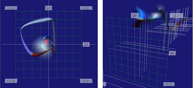
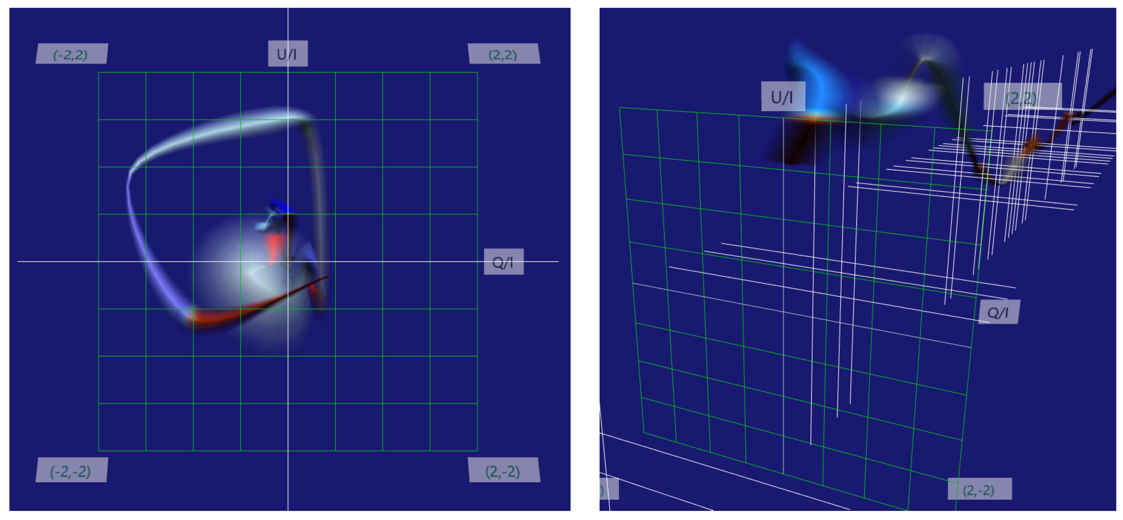
2. TimeTubes

We consider the time-series data of the total flux, color, and fractional Stokes parameters $(Q/I,U/I)$. In this article, we use not $(Q,U)$, but the fractional values, because the variations in polarization are emphasized. Of course, TimeTubes can also be used for $(Q,U)$. Figure 1 shows the light curve, color–magnitude diagram, and polarization data plots on the Stokes $(Q/I,U/I)$ plane for 3C 66A observed with the Kanata telescope [5]. The red points in each panel indicate the data taken on the same night. Such views are ineffective when searching for noteworthy patterns of the trajectory in the $(Q/I,U/I)$ plane which correlate with the flux and color.

A visualization tool, “TimeTubes” has been developed for the polarization variations in blazars [9]. In TimeTubes, the trajectory is visualized in 3D space with the time axis as the third axis, in addition to the 2D $(Q/I,U/I)$ plane. We express the trajectory as “tubes” in this 3D space. Figure 2 shows an example of the TimeTubes view for the data of 3C 66A, around MJD 52000 when a rapid flare was observed. The center of the tube corresponds to the observed $Q/I$ and $U/I$. The widths of the tube represent the measurement errors. Figure 3 shows the color map for the tube. Using this 2D color map, the observed color and flux are visualized as the tube’s color. As a result, we can see six variables ($Q/I$, $U/I$, their errors, flux, and color) in one TimeTubes view. In Figure 2, we can see a brightening and bluing period; that is, a flare with a variation in polarization.

TimeTubes is still under development. Some useful functions which are currently available are described as follows: (i) The temporal progress can be controlled with the mouse wheel, while we can jump to any given times using the “Time Search” function; (ii) The scales of the color map can be adjusted for any given ranges; (iii) The data with large errors can be located by different colors using the “Outlier filtering” function; (iv) The appearance of the tube can be adjusted from solid-like to blurring structures by using the “Opacity transfer function editor”; (v) The data can also be shown in the classical scatter plots. More details are available in [9].

3. Applications to Real Data

In this section, we introduce examples of the TimeTubes view for the data of PKS 1749+096 and 3C 454.3 taken with the Kanata telescope [5].

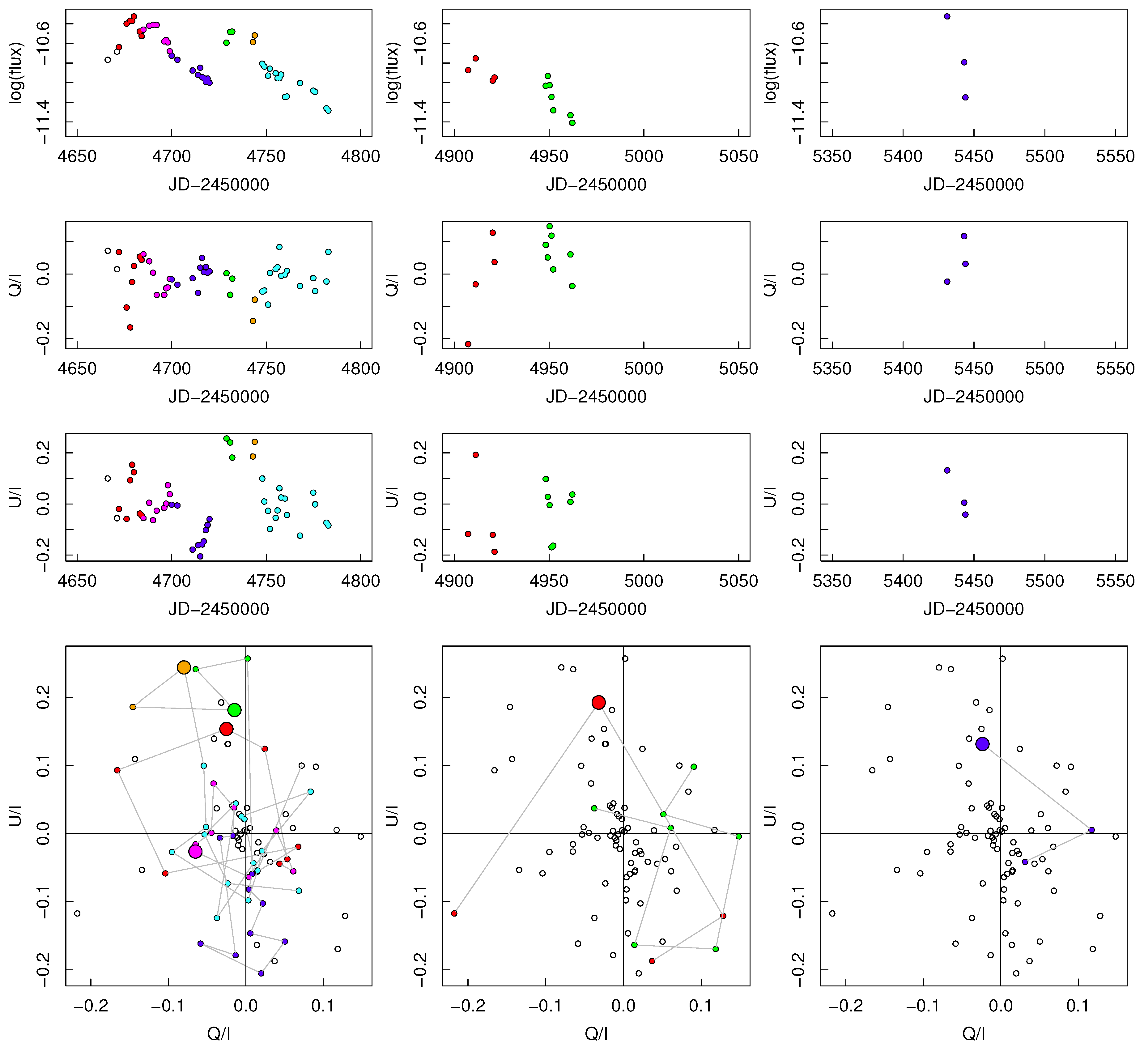
3.1. PKS 1749+096

Figure 4 is the TimeTubes view of PKS 1749+096 around MJD 54675 (left panel) and MJD 54730 (right panel). In the left panel, we can see a clear rotation feature, which was observed for 12 days. The rotation begins from a low region of the $QU$ plane and occurs in the clock-wise direction. Owing to TimeTubes, we can quickly recognize that the flare and color variation are associated with the rotation; the object starts with a dark-red state, then becomes brighter and bluer, and reaches the brightest state at a high $U/I$ region.

The right panel of Figure 4 shows the TimeTubes view ∼50 d after the rotation event. Two other flares can be identified with the bright and light-blue colored parts of the tubes. These two flares have similar polarization vectors; that is, large $U/I$ and small $Q/I$. Now, we find that the flare associated with the rotation also has a similar polarization direction at its peak. Those three flares suggest that flares of this object tend to have a common polarization direction. Then, we investigate this idea by using the other data of this object with more standard plots.

Figure 5 shows the V-band light curves (upper) and $(Q/I,U/I)$ planes (lower). The left, middle, and right panels are those in 2008, 2009, and 2010, respectively. The data in the left panel covers those shown in Figure 4. The light curve in 2008 is divided into five parts indicated by the different colors. The colors of the points in the $(Q/I,U/I)$ plane correspond to those in the light curve. There are two major outbursts which have multiple peaks; that is, the first outburst between MJD 54670 and 54730 (the red, magenta, and blue points), and the second one between MJD 54730 and 54780 (the light-green, orange, and cyan points). The observed peaks of the flares are indicated by the large circles in the lower panel.

We confirm that the flare was associated with the rotation, as indicated by the red points in the left panel. In 2008, we detected four flares as indicated by the red, magenta, light-green, and orange points. We confirm that three flares (with the exception of the magenta one) have a common polarization direction. In 2009, no bright state was detected in our observations, while the brightest point in this year is emphasized as the large red symbol in the $(Q/I,U/I)$ plane. In 2010, we again detected a bright flare. While the data was poor, the brightest point in 2009 and flare in 2010 seem to have a common polarization direction, as can be seen in the middle and right panels of Figure 5. In total, four flares out of five have a common polarization direction. In addition, three flares, including a possible one in 2009, exhibit large variations in PA around the flare peaks. They imply that polarization rotation is also common in the flares of this object.

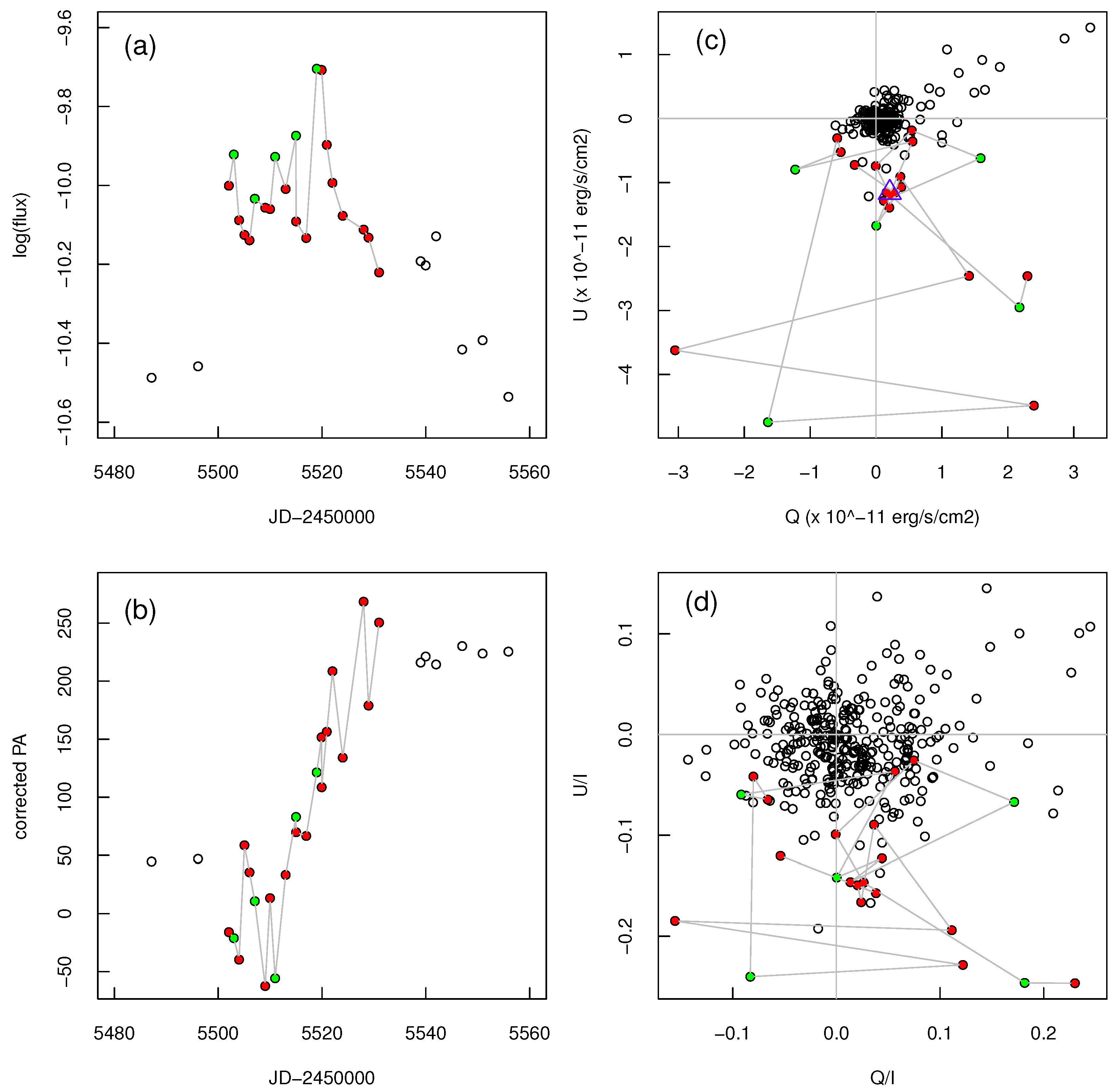
3.2. 3C 454.3

Figure 6 shows the TimeTubes view of 3C 454.3 around MJD 55510. The color parameter of the tubes, that is—the value of the horizontal axis of the color map in Figure 3—is fixed, since we have no color data in this period of time. The polarization variation is quite complicated. On the other hand, we can see that the object repeats bright and faint states, and furthermore that the polarization direction of the bright states appears to rotate in the anti-clockwise direction, centering on a negative $U/I$ and small $Q/I$ area. TimeTubes helped us to find this noteworthy pattern, and thereby triggered us to investigate it more carefully in the standard plots.

Figure 7 shows (a) the light curve, (b) PA, (c) the Stokes $(Q,U)$, and (d) $(Q/I,U/I)$ planes. The data shown in Figure 6 corresponds to the period indicated by the red points. The object was in an active state throughout this period, and experienced small flares, as can be seen in the light curve. The light-green points are the peaks of the flares. In the Stokes planes, the blue open triangle indicates medians of $QU$ in the active state: $(Q_m,U_m)=(+0.21,-1.16)(\times {10}^{11}\mathrm{erg}·{\mathrm{s}}^{-1})$. The object exhibits violent variations, while it stays around $(Q_m,U_m)$ before/after each flare when the object is relatively faint. We calculated PA values centering on this blue point, and plotted them in panel (b) of Figure 7. Then, we can see a systematic increase in the corrected PA during the active state.

4. Discussion and Summary

In the last section, we introduced the TimeTubes view of two blazars and compared them with more standard plots, like light curves, time-series of PA, and the Stokes planes. Both features of PKS 1749+096 and 3C 454.3 were first noticed in the TimeTubes views, and then confirmed in more standard plots. These results demonstrate that TimeTubes helps us to find interesting patterns in the polarization data of blazars. In this section, we first discuss astrophysical implications of the two examples, and then comment on the future plans of TimeTubes.

PKS 1749+096 is a BL Lac object classified as LBL [10]. As mentioned in the last section, the optical PA is distributed over a wide range, while the peaks of flares tend to have a common direction of PA $=+{50}^{\circ }$–$+{60}^{\circ }$. The polarization rotation also follows this trend. This favored PA is close to the position angle of the radio jet in its downstream region ($+{30}^{\circ }$–$+{50}^{\circ }$) [11]. A scenario with the spiral path of the shocked region through a toroidal magnetic field is proposed to explain the polarization rotations [3]. Those observations suggest that a geometrical effect makes the flare peaks. We propose that the flares reached their peak at the time when the beaming factor becomes maximum, while the flares themselves are probably due to the moving shocks in the spiral path.

3C 454.3 is a famous flat spectrum radio quasar (FSRQ). In the last section, we reported a polarization rotation episode of the consecutive flares. A similar event was reported in the same object in 2007, in which the average polarization vectors of at least five flares exhibited a rotation-like feature within 80 d in that event [12]. The situation is also similar to the long-term polarization rotation of PKS 1510-089 observed in 2009, when the object was active, and a number of short flares were observed during the rotation episode [4]. The rotation that we detected is centered not on the origin of $(Q,U)$, but on $(Q_m,U_m)$. The polarization component of $(Q_m,U_m)$ is probably a component of the active state. It is hard to find such an off-axis rotation in the standard plots, such as a time-series plot of PA, making it a good example to demonstrate the advantage of TimeTubes.

More detailed reports about the above two observations will be published in forthcoming papers.

In this article, we demonstrated how we obtained new insights through a visualization tool for the blazar polarization, TimeTubes. This approach to handle the data is crucial for the study of blazar variations with polarization when the data size is large. Even in the case of small data sets, to use TimeTubes is an effective way to find interesting features in the data. TimeTubes is still an ongoing project. We have a plan to add more functions for better usage. In particular, a dynamic connection between the TimeTubes view and scatter plots will be quite useful for our analysis. One can download the current version of TimeTubes at our project page: http://fj.ics.keio.ac.jp/index.php/projects/spm/. The functions of TimeTubes are described in [9].

References

- Hagen-Thorn, V.A.; Larionova, E.G.; Jorstad, S.G.; Björnsson, C.-I.; Larionov, V.M. Analysis of the long-term polarization behaviour of BL Lac. Astron. Astrophys. 2002, 385, 55–61. [Google Scholar] [CrossRef]
- Abdo, A.A.; Ackermann, M.; Ajello, M.; Axelsson, M.; Baldini, L.; Ballet, J.; Barbiellini, G.; Bastieri, D.; Baughman, B.M.; Bechtol, K.; et al. A change in the optical polarization associated with a γ-ray flare in the blazar 3C 279. Nature 2010, 463, 919–923. [Google Scholar] [CrossRef] [PubMed]
- Marscher, A.P.; Jorstad, S.G.; D’Arcangelo, F.D.; Smith, P.S.; Williams, G.G.; Larionov, V.M.; Oh, H.; Olmstead, A.R.; Aller, M.F.; Aller, H.D.; et al. The inner jet of an active galactic nucleus as revealed by a radio-to-γ-ray outburst. Nature 2008, 452, 966–969. [Google Scholar] [CrossRef] [PubMed]
- Marscher, A.P.; Jorstad, S.G.; Larionov, V.M.; Aller, M.F.; Aller, H.D.; Lähteenmäki, A.; Agudo, I.; Smith, P.S.; Gurwell, M.; Hagen-Thorn, V.A.; et al. Probing the Inner Jet of the Quasar PKS 1510-089 with Multi-Waveband Monitoring During Strong Gamma-Ray Activity. Astrophys. J. Lett. 2010, 710, L126–L131. [Google Scholar] [CrossRef]
- Ikejiri, Y.; Uemura, M.; Sasada, M.; Ito, R.; Yamanaka, M.; Sakimoto, K.; Arai, A.; Fukazawa, Y.; Ohsugi, T.; Kawabata, K.S.; et al. Photopolarimetric Monitoring of Blazars in the Optical and Near-Infrared Bands with the Kanata Telescope. I. Correlations between Flux, Color, and Polarization. Publ. Astron. Soc. Jpn. 2011, 63, 639–675. [Google Scholar] [CrossRef]
- Pavlidou, V.; Angelakis, E.; Myserlis, I.; Blinov, D.; King, O.G.; Papadakis, I.; Tassis, K.; Hovatta, T.; Pazderska, B.; Paleologou, E.; et al. The RoboPol optical polarization survey of gamma-ray-loud blazars. Mon. Not. R. Astron. Soc. 2014, 442, 1693–1705. [Google Scholar] [CrossRef]
- Smith, P.S.; Montiel, E.; Rightley, S.; Turner, J.; Schmidt, G.D.; Jannuzi, B.T. Coordinated fermi/optical monitoring of blazars and the great 2009 September Gamma-ray flare of 3C 454.3. In Proceedings of the 2009 Fermi Symposium, Washington, DC, USA, 2–5 November 2009.
- Uemura, M.; Kawabata, K.S.; Sasada, M.; Ikejiri, Y.; Sakimoto, K.; Itoh, R.; Yamanaka, M.; Ohsugi, T.; Sato, S.; Kino, M. Bayesian Approach to Find a Long-Term Trend in Erratic Polarization Variations Observed in Blazars. Publ. Astron. Soc. Jpn. 2010, 62, 69–80. [Google Scholar] [CrossRef]
- Xu, L.; Nakayama, M.; Wu, H.-Y.; Watanabe, K.; Takahashi, S.; Uemura, M.; Fujishiro, I. TimeTubes: Design of a Visualization Tool for Time-Dependent, Multivariate Blazar Datasets. In Proceedings of the NICOGRAPH International 2016, Hangzhou, China, 6–8 July 2016.
- Abdo, A.A.; Ackermann, M.; Agudo, I.; Ajello, M.; Aller, H.D.; Aller, M.F.; Angelakis, E.; Arkharov, A.A.; Axelsson, M.; Bach, U.; et al. The Spectral Energy Distribution of Fermi Bright Blazars. Astrophys. J. 2010, 716, 30–70. [Google Scholar] [CrossRef]
- Lu, R.-S.; Shen, Z.-Q.; Krichbaum, T.P.; Iguchi, S.; Lee, S.-S.; Zensus, J.A. The parsec-scale jet of PKS 1749+096. Astron. Astrophys. 2012, 544, A89. [Google Scholar] [CrossRef]
- Sasada, M.; Uemura, M.; Arai, A.; Fukazawa, Y.; Kawabata, K.S.; Ohsugi, T.; Yamashita, T.; Isogai, M.; Nagae, O.; Uehara, T.; et al. Multiband Photopolarimetric Monitoring of an Outburst of the Blazar 3C 454.3 in 2007. Publ. Astron. Soc. Jpn. 2010, 62, 645–652. [Google Scholar] [CrossRef]
© 2016 by the authors; licensee MDPI, Basel, Switzerland. This article is an open access article distributed under the terms and conditions of the Creative Commons Attribution (CC-BY) license (http://creativecommons.org/licenses/by/4.0/).
Share and Cite
Uemura, M.; Itoh, R.; Xu, L.; Nakayama, M.; Wu, H.-Y.; Watanabe, K.; Takahashi, S.; Fujishiro, I. TimeTubes: Visualization of Polarization Variations in Blazars. Galaxies 2016, 4, 23. https://doi.org/10.3390/galaxies4030023
Uemura M, Itoh R, Xu L, Nakayama M, Wu H-Y, Watanabe K, Takahashi S, Fujishiro I. TimeTubes: Visualization of Polarization Variations in Blazars. Galaxies. 2016; 4(3):23. https://doi.org/10.3390/galaxies4030023
Chicago/Turabian StyleUemura, Makoto, Ryosuke Itoh, Longyin Xu, Masanori Nakayama, Hsiang-Yun Wu, Kazuho Watanabe, Shigeo Takahashi, and Issei Fujishiro. 2016. "TimeTubes: Visualization of Polarization Variations in Blazars" Galaxies 4, no. 3: 23. https://doi.org/10.3390/galaxies4030023
APA StyleUemura, M., Itoh, R., Xu, L., Nakayama, M., Wu, H.-Y., Watanabe, K., Takahashi, S., & Fujishiro, I. (2016). TimeTubes: Visualization of Polarization Variations in Blazars. Galaxies, 4(3), 23. https://doi.org/10.3390/galaxies4030023