IFU Spectroscopic Study of the Planetary Nebula Abell 30: Mapping the Ionisation and Kinematic Structure of the Inner Complex

Abstract

This work presents integrated flux and velocity channel maps of the planetary nebula Abell 30 (A30) inner knot system. The observations were taken with the INTEGRAL spectrograph at the William Herschel Telescope (WHT), La Palma, Spain. Our IFU data cube has a field of view (FoV) of 12.3″× 16″ that partially covers knots J1 and J2, and completely covers knots J3 and J4 in the system. Optical Recombination Lines (ORLs) of C II, He I, He II, N III, O II and Collisionally Excited Lines (CELs) of [Ar IV], [Ar V], [N II], [Ne III], [Ne IV], and [O III] were detected. Our integrated flux maps visualise the ionisation structure and the chemical inhomogeneity in the system previously reported by other groups. We find that ORLs are concentrated in the polar region (J1, J3), whereas the equatorial knots (J2, J4) are dominated by CELs. The flux ratio map of the diagnostic [O III $\lambda$ 5007/4363 Å] lines reveals the electron temperature distribution, which shows cold cores of 15,000 K in knots J3 and J4 surrounded by a hot outer layer of above 20,000 K. Our channel maps show positive and negative velocity excursions from the systemic value among the ions. Several ions show variation in their velocity structures from their lower-energy-level counterparts, including [Ar IV] and [Ar V], [Ne III] and [Ne IV], and He I and He II. New recurrent velocity structures are identified in the low-density regions where the ions move much faster compared to their surrounding environments. The velocity dispersion measurements highlight extreme turbulence in some of the ions (${\sigma }_{{\mathrm{v}}_{\mathrm{rad}}}\approx 140$ km/s), consistent with supersonic/hypersonic motion driven by shocks. The forbidden line species [N II] exhibits lower turbulence (${\sigma }_{{\mathrm{v}}_{\mathrm{rad}}}\approx$ 50–60 km/s), tracing denser, less-turbulent gases. Based on our data, we conclude that both the ionisation and kinematic studies hint at shock heating and multiple ejection history in the evolutionary pathway of A30.

1. Introduction

Abell 30 (A30) is a well-known and interesting planetary nebula (PN) that has a few different nomenclatures, e.g., PNG 208.5 + 33.2. It was known as PN A66 30 when it was first discovered in 1964 [1,2].

A30 belongs to a highly ionised PN class arising from its very hot core. In the work of Jacoby [3], it was emphasised that A30 had a hydrogen-rich outer shell and a hydrogen-poor inner knot system in close proximity to the central star. This is rare in PNe systems [3]. A secondary envelope ejection was suspected as being responsible for the inner hydrogen-poor nebula [4]. Jacoby and Ford [5] suggested the possibility of a binary companion which gained observational support by the detection of a variable light curve with a period of 1.060 days discovered in 2020 [6]. The binary system in A30 is one of the proposed mechanisms to explain the chemical inhomogeneity observed in the inner knot system via the possible existence of an accretion disk from binary interaction [7]. Recent studies of the equatorial knots include refs. [8,9], which reveal the presence of dust in the equatorial region.

In general, a main sequence star of mass ranging from 1 to 8 solar masses will only eject its outer atmospheric layer once the object enters the AGB phase. The ejected material then becomes ionised by the hot core, causing it to glow in emission lines across much of the electromagnetic spectrum. This short evolutionary stage is collectively known as the PN phase. Its typical life span is about 5000–25,000 years [10]. PNe systems are generally hydrogen-rich [11]. Observational data for A30 suggests an interval of 12,000–18,000 years between the first and second ejection of the outer hydrogen-rich nebular shell and the inner hydrogen-deficient knot system [3,12], making it an outlier relative to the usual low-mass star evolutionary pathway.

The origin of chemically inhomogeneous ejecta in the inner knot system remains uncertain, and several theories have been proposed over the years. In the single-star scenario, a late-stage eruption via a Very Late Thermal Pulse (VLTP) [13,14] and subsequent born-again event [15] explains the extreme abundance contrast between the H-rich outer nebula and the H-poor, C/O-rich knots surrounding the central star. Alternatively, the binary-star scenario involves multiple ejections modulated by a companion star [5,7], including common envelope evolution [16], to produce the observed clumpy, chemically distinct knots. The latest observational evidence clearly favours the binary scenario.

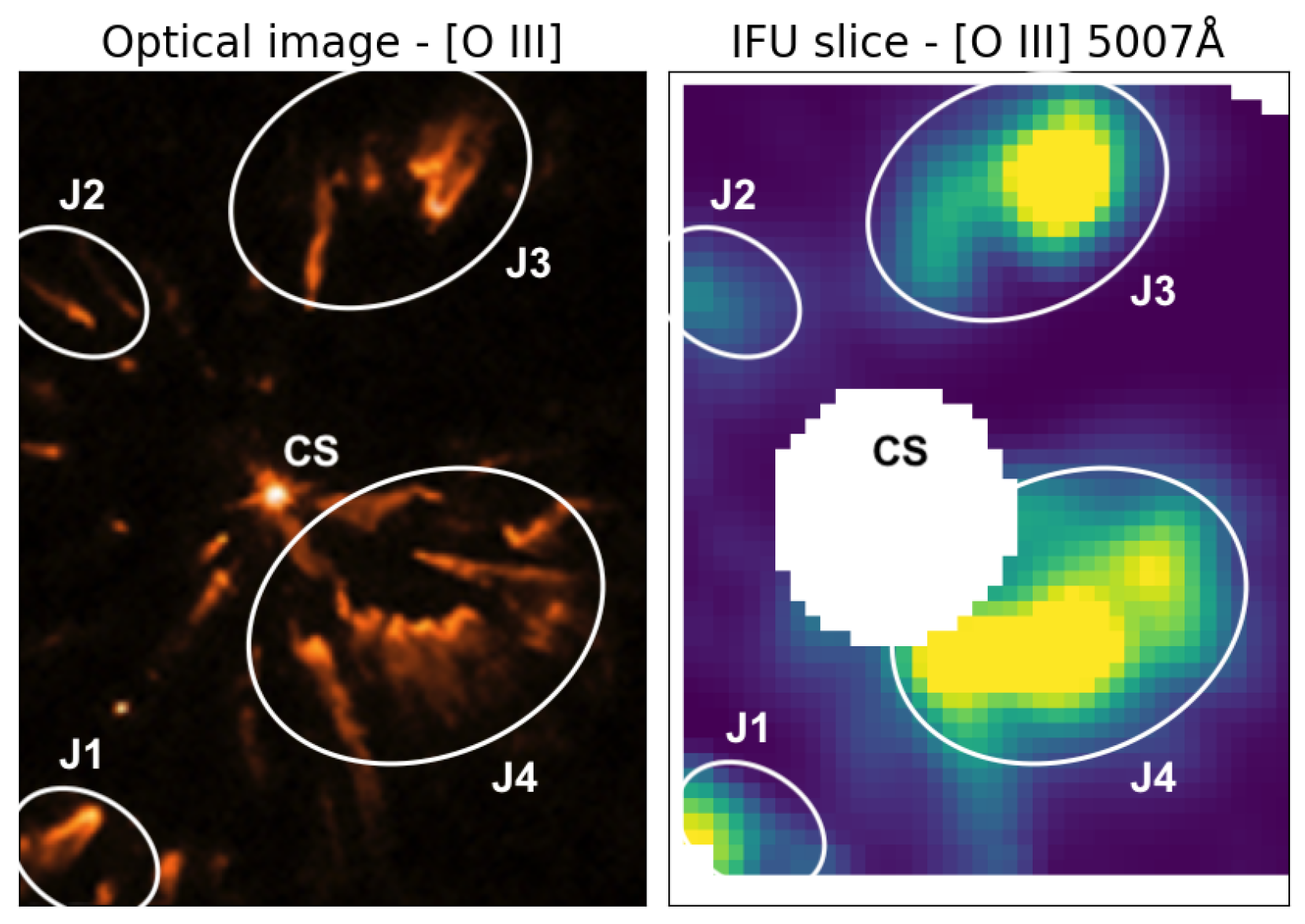
The hydrogen-poor inner knot system of A30 referred to in this work is divided into four main parts. These are knots J1, J2, J3, and J4 (Figure 1), starting from the SE nebula structure and counting clockwise around the central star [3]. Knots J2 and J4 are collectively known as the equatorial system and knots J1 and J3 as the so-called polar knots.

Here, we present an IFU spectroscopic study for A30 to investigate the distribution of ionic species across the gas clumps in the inner knot system and the kinematic structure observed in a series of spectral lines. Our integrated flux maps visualise the ionisation structure of detected ions that originates from various transitions taking place across the system. The channel maps and velocity structure visualised in our study support the multiple ejecta scenario or a complex outflow based on the varying Doppler shifts observed across different ions in the system.

2. Observations

Observations were taken using the INTEGRAL [18] integral field unit (IFU) 2D spectroscopic facility of the William Herschel Telescope in combination with the WYFFOS spectrograph. “Fibre bundle 2” with a FoV of 12.3$″$× 16$″$ was used with an individual fibre size of 0.9$″$. Note that the 219 fibres are not spatially contiguous because approximately 40% of the total FoV falls into the gaps between the fibres. A ring of 30 fibres offset by 45$″$ from the centre of the FoV allows the sky spectrum to be obtained simultaneously. The observations reported here were taken in 2004 (January 14) by Katrina Exter (PI) and were approximately centred on the central star of A30, fully covering the knots J4 and J3, and part of the equatorial knot J2 and the polar knot J1. Seeing was reported as ≤1$″$. Six 1800 s observations with each of the red and blue 1200 l mm⁻¹ gratings were taken, covering the spectral range of 3800–5230 Å in the blue and 5170–6600 Å in the red. Our IFU data cubes are composites of 1001 slices with a wavelength spacing of 1.47 Å in the blue and red.

Bias subtraction, spectral identification, tracing, and extraction of the raw CCD data were performed within IRAF. Cosmic rays were removed with a median-combination technique (with $\sigma$-rejection) using images in groups of three, supplemented occasionally by manual intervention. The wavelength calibration was performed using spectra extracted from CuAr + CuNe arc calibration lamp frames. Due to the absence of arc emission lines below 4300 Å in the blue spectra, we re-calibrated those spectra using the measured positions of the PN emission lines reported in [19] for knots J1 and J3. We note that for the red spectra, our measured line positions show an offset of ≈1 Å compared to the positions stated in [19] (their wavelengths being smaller); however, the velocity maps from our wavelength calibration are more consistent between the blue and red arms for the individual line species (see below).

3. Data Cubes

Because all spectra were slightly offset with respect to each other, we converted the individual spectra (from 0.9$″$ round spaxels with 40% in gaps) into data cubes (with 0.3$″$ spaxels with no gaps and a square grid) using the spatial interpolation routine provided by the “Euro 3D visualisation tool” [20]. The core of this process is to resample the input spatial grid (which is the sky footprint of INTEGRAL) onto a new, contiguous, and regular grid, using “Delaunay” triangulation to select the best grid points. The fluxes are then interpolated from the input grid to the output grid at each wavelength in the dataset; we adopted the natural-neighbour flux-conserving interpolation method. The central star is a sufficiently bright source to trace the Differential Atmospheric Refraction (DAR) with wavelength, even though the PSF is not very well sampled [21]. After correcting for the DAR, the six red and blue cubes were combined into the final data cubes.

4. Spectral Analysis—Integrated Flux Maps

Abell 30 has been extensively studied for its asymmetric chemical distribution across the inner knot system, with various groups exploring the X-ray, UV, visible, IR, and FIR spectral ranges (e.g., [22,23,24]). In the visible range, refs. [5,12] and subsequent studies by refs. [8,19] reported the presence of ORLs and CELs (or forbidden lines, demarcated by brackets []) of Oxygen (O II, [O II], and [O III]), Neon ([Ne III], [Ne IV], and [Ne V]), Nitrogen ([N II] and N III), Helium (He I and He II), Carbon (C II and C III), Sulfur ([S II]), Argon ([Ar IV], [Ar V]), as well as trace amounts of Hydrogen (${\mathrm{H}}_{\alpha }$ to ${\mathrm{H}}_{\gamma }$). Furthermore, ref. [9] studied the carbon-rich dust and detected lines of heavier elements including Fe V, Mg I, and [Na II] in the IR spectra, likely sourced from the equatorial region. Due to the presence of high-excitation emission lines, A30 is classified as a member of the high-excitation PNe.

Our spectral analysis focuses on the inner knot system within a 12.3$″$× 16$″$ FoV. Python 3.9 packages including PyNeb1 [25] were used for the emission line analysis. The flux calibrated spectra of the individual spaxels were corrected for the heliocentric velocity and de-reddened using the extinction law of [26], adopting a value of c(${\mathrm{H}}_{\beta }$) = 0.6 from [19], followed by continuum subtraction. To extract the ionisation structure information from our IFU data cube, the central star as well as the background star to the South–East of it were masked.

For each un-blended spectral line detected, due to the skewed instrumental line profiles, we integrated the flux density over the corresponding wavelength range (${\lambda }_0\pm 6$ Å) to produce one single flux map. Individual fluxes of different lines from the same ion were then added to produce the final flux maps as shown in Figure 2, Figure 3, Figure 4, Figure 5, Figure 6 and Figure 7. These maps visualise the ionisation structures of different ions distributed across the inner knot system that originate from various electron transitions.

Table 1. Ion species with ionisation energies needed to produce the ion and integrated fluxes of each species for each normalised knot, so [O III] in J4 is 10,000. Ions are sorted by their ionisation energies. Note that the different sizes of the knots influence the integrated fluxes, which may differ from the perceived strengths in the maps. Only J3 and J4 are fully covered by our FoV.

Ion	Ionisation Energy [eV]	J1	J2	J3	J4
He I	0	89	19	391	233
C II	11.3	27	4	95	32
O II	13.6	17	0	59	14
[N II]	14.5	30	11	152	396
He II	24.6	219	96	793	812
N III	29.6	11	4	33	13
[O III]	35.1	882	783	4503	10,000
[Ar IV]	40.7	1	4	5	15
[Ne III]	41.0	156	144	784	1986
[Ar V]	59.4	1	1	4	14
[Ne IV]	63.5	20	57	71	337

shows the sum of fluxes for the individual ions and knots, scaled so that the strongest line ([O III] in knot J4) has a strength of 10,000. The ORLs of low-to-medium ionisation energy ions mainly populate the polar knots J1 and J3 while the equatorial knots J2 and J4 are dominated by the CELs of high-ionisation energy species. The only recombination lines which can clearly be seen in the equatorial knot J4 are from Helium (He I and II) atoms.

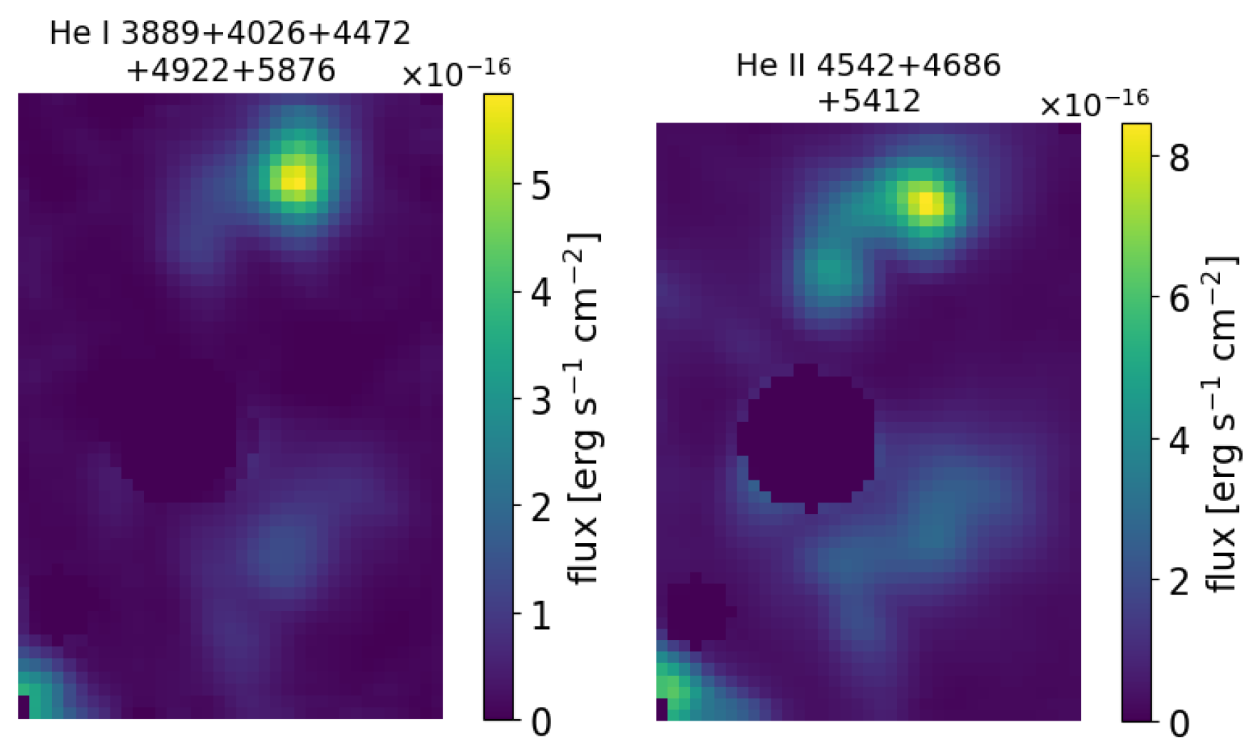
Neutral and singly ionised Helium lines mainly populate the polar knots J1 and J3, with traces to be found in J4 (Figure 2). He II lines appear slightly stronger in the South–East extension of J3 as well as in J4 compared to He I.

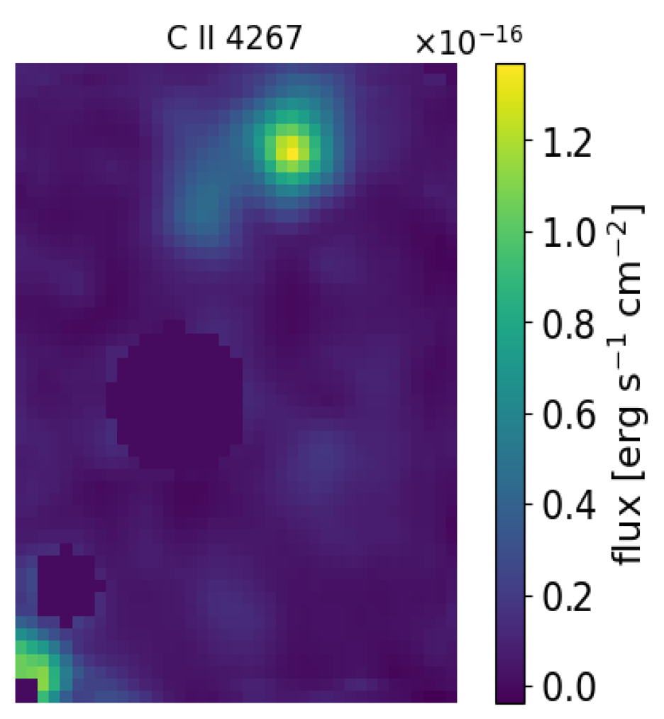
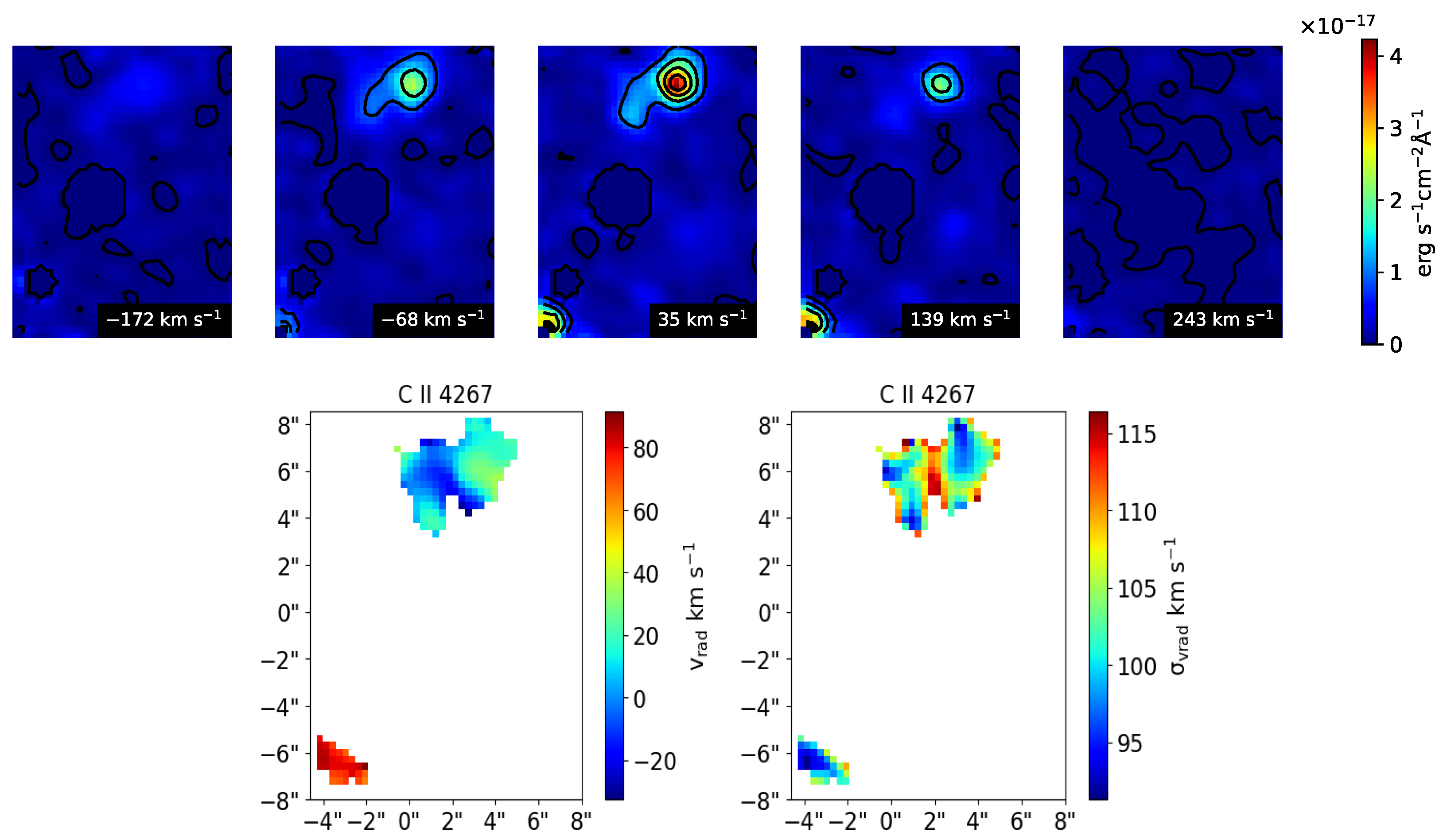
The ORL of C II (4267 Å, Figure 3, left) is only visible in the polar knots J1 and J3.

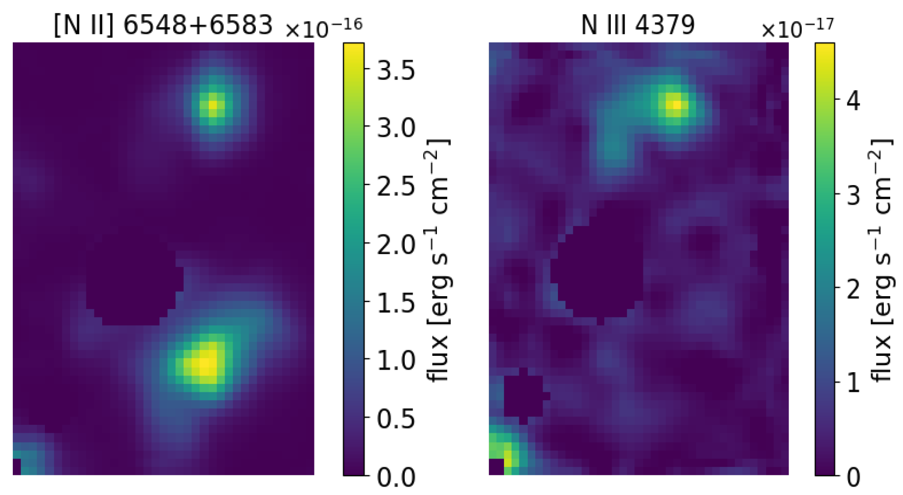
The forbidden singly ionised Nitrogen species ([N II] 6548 Å and 6583 Å, same upper and lower energy levels) covers knots J3 and J4 (see Figure 4, left and centre) and are fainter in J1. However, ORLs of N III (4379 Å, Figure 4, right) with twice the ionisation potential are only present in the polar knots J1 and J3. While [N II] is concentrated in the North–West part of J3, N III is also visible in the South–East extension of J3.

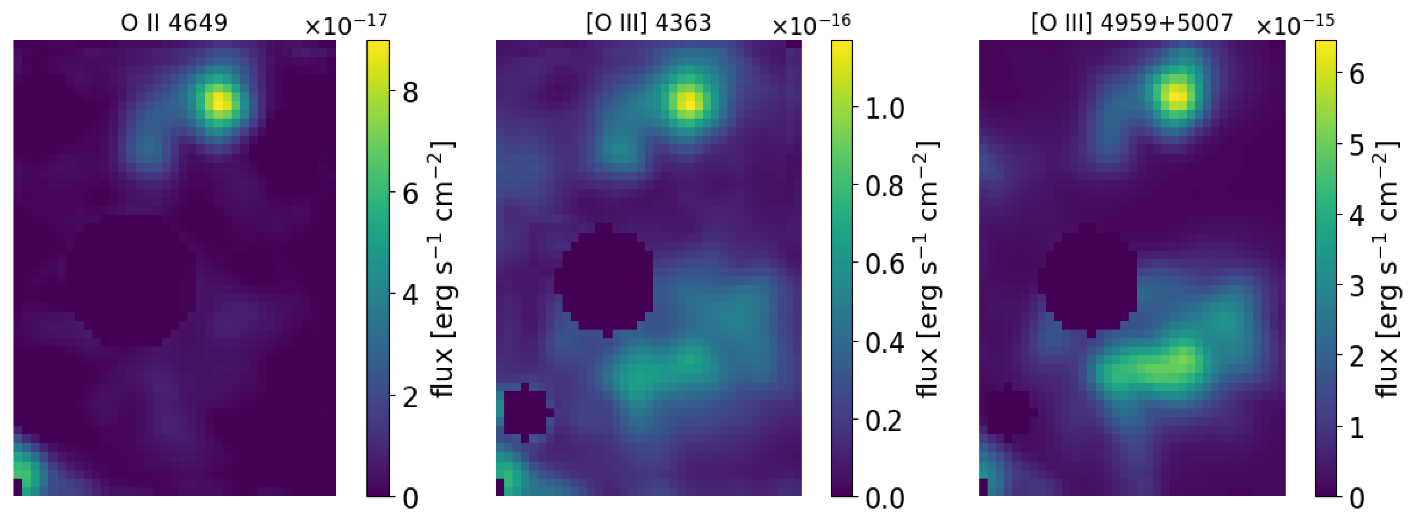
O II (Figure 5, left panel) is also predominantly present in J1 and J3, while the forbidden [O III] lines can also be found in J2 and J4 (Figure 5 centre and right panels).

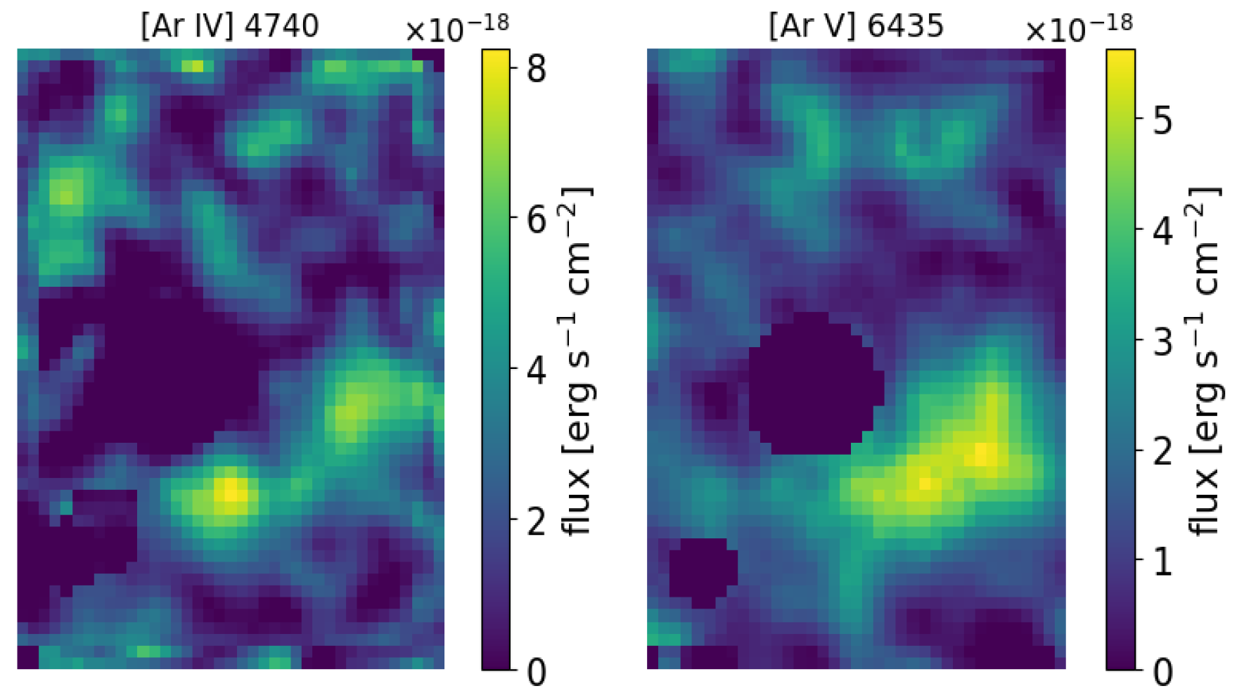
The high-ionisation species [Ar IV] and [Ar V] are very weak and noisy; however, it is clear that [Ar IV] (Figure 6, left panel) appears strongest in the equatorial knots J2 and J4, while [Ar V] with an ionisation energy 1.5 times stronger appears to be only present in J4 (Figure 6, right panel).

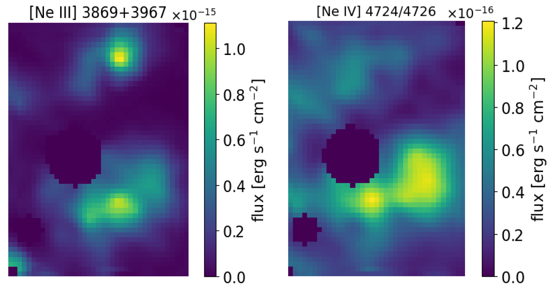
CELs of doubly ionised Neon ([Ne III] 3869 Å and 3967 Å, both representing transitions from the same upper level to the same lower level; see Figure 7, left) are found both in the polar and equatorial knots. In contrast, its higher-ionisation counterpart [Ne IV] (63.4 eV; unresolved doublet 4724/4726 Å; see Figure 7, right) that has a 1.6 times greater ionisation potential is predominantly found in the equatorial knots, especially knot J4.

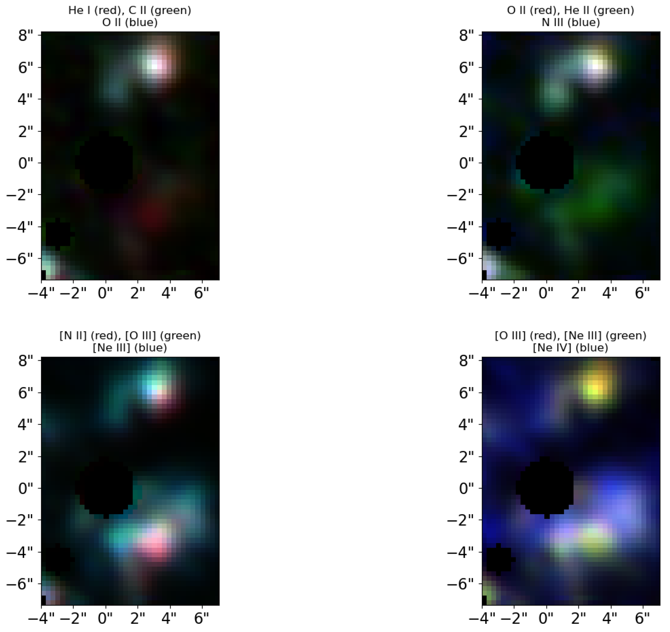
Combinations of the 3 lowest and 3 highest ionisation species for ORLs and CELs individually are shown in (Figure 8). Knot J4 is dominated by CELs with only a weak and diffuse contribution of He lines. Additionally, it appears that the lower-ionisation species are more concentrated compared to the higher-ionisation species, which are more diffuse. ORLs are produced predominantly in the polar knots J1 and J3 and partially in knot J4 of the equatorial knots. CELs of low- and high-ionisation-level species dominate the equatorial regions—J2 and J4.

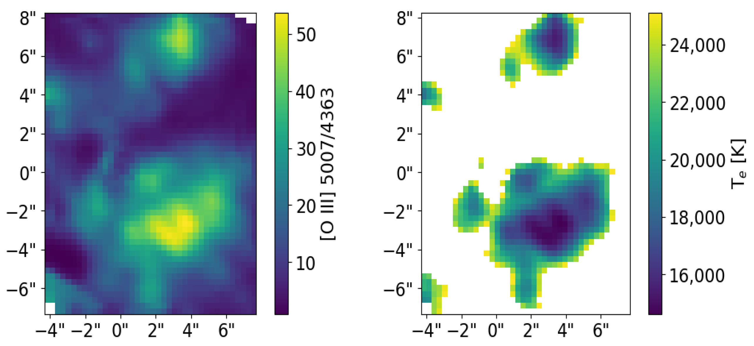
Our map of the electron temperature distribution (Figure 9, right panel) was derived from the [O III] line ratios 5007/4363 (Figure 9, left panel). Ref. [19] state electron densities of 2800 and 3200 cm⁻³ for the knots J1 and J3, respectively, which are the highest values obtained in the literature. However, even with these high values we are safely in the low density regime and assumed electron densities of 3000 cm⁻³ for the creation of our temperature map. Knots J3 and J4 exhibit a cool core ($T_e\simeq 15,000$ K) surrounded by a hot outer layer of above 20,000 K, which is in good agreement with previously determined averaged temperatures by [5,8,12] as well as the proposed existence of cold cores surrounded by much hotter outer regions of the knots [19,23]. Knots J1 and J2 are only partially covered so no statement about a possible cool core and hot shell can be made here. The presence of cool cores may indicate shielding from the central star’s radiation, possibly by dust [23], or shock heating in the outer envelopes of the high-density knots.

5. Kinematic Structure and Velocity—Multiple Kinematic Components

The outer shell of A30 expands at a velocity of about 30–40 $\mathrm{km}{\mathrm{s}}^{-1}$ while the inner knots show complex structures with velocity spikes of ±200 $\mathrm{km}{\mathrm{s}}^{-1}$ [27,28].

The spectral resolution of our data ranges from R ≈ 1650 at 3800 Å to R ≈ 2700 at 5200 Å for the blue arm and R ≈ 2100 to 3600 for the blue and red ends of the red arm, respectively. Doublets that are less than 3 Å apart are therefore not resolved in our data, as is the case for [Ne IV] 4725.5/4726.9 Å, leading to broadened line profiles. The spectral resolution is equivalent to a velocity resolution of ≈180 $\mathrm{km}{\mathrm{s}}^{-1}$ at the blue end and ≈80 $\mathrm{km}{\mathrm{s}}^{-1}$ at the red end. Discrete sampling intervals (sampling widths) of each slice are ≈115 $\mathrm{km}{\mathrm{s}}^{-1}$ for the blue end and ≈70 $\mathrm{km}{\mathrm{s}}^{-1}$ for the red end, which give sample ratios of ≈1.57 to 1.14, respectively, which is lower than the Nyquist-compliant sampling requirement of ≥2 [29]. Therefore, velocity analysis in the kinematic studies of this work is focusing on kinematic structure. All velocities derived in this study are based on the laboratory wavelength.

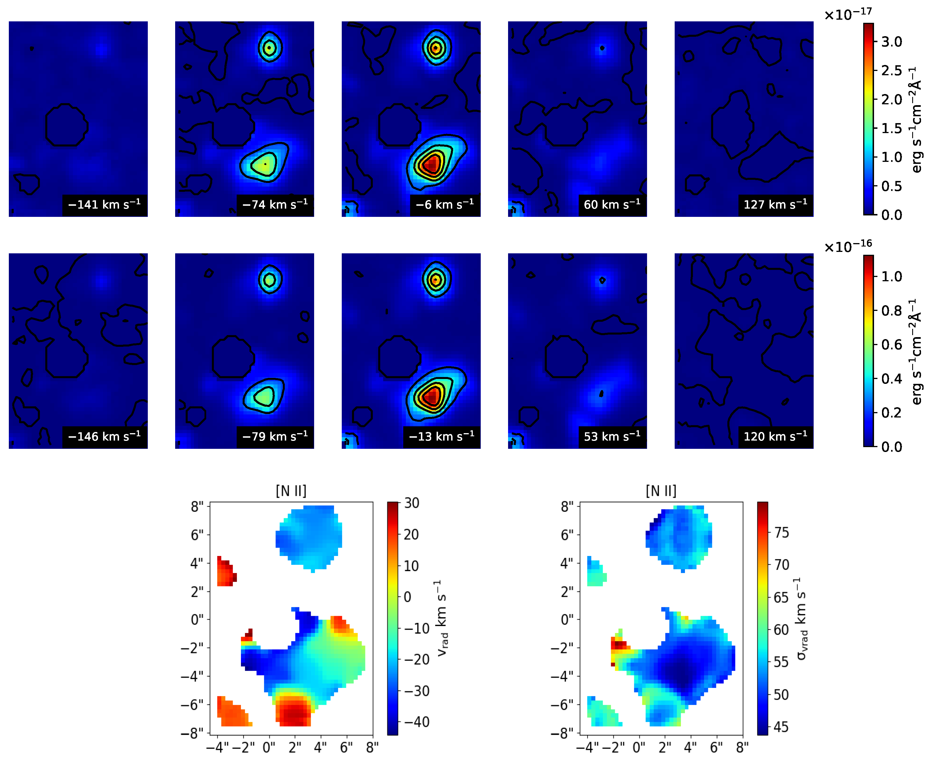
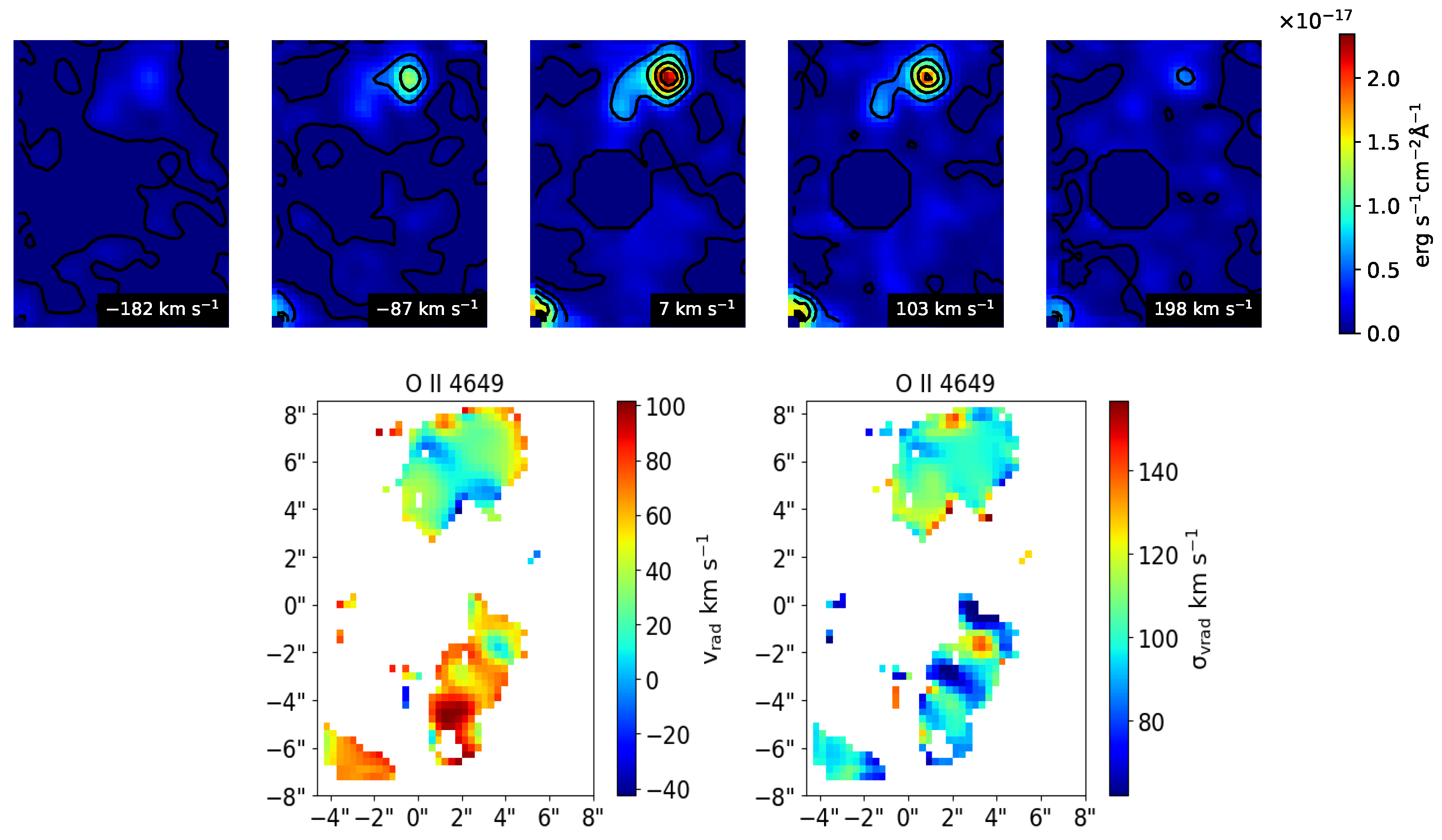
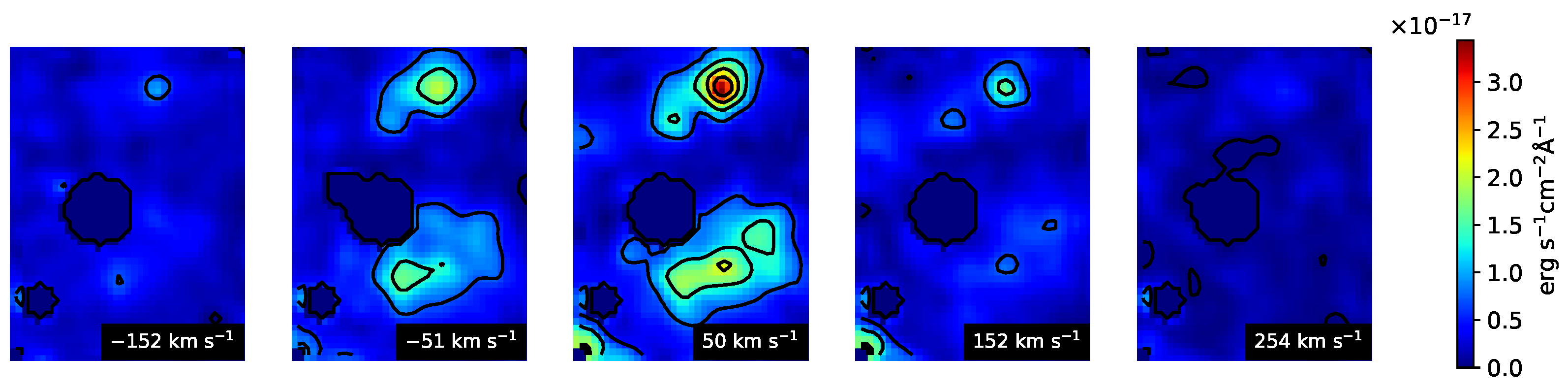
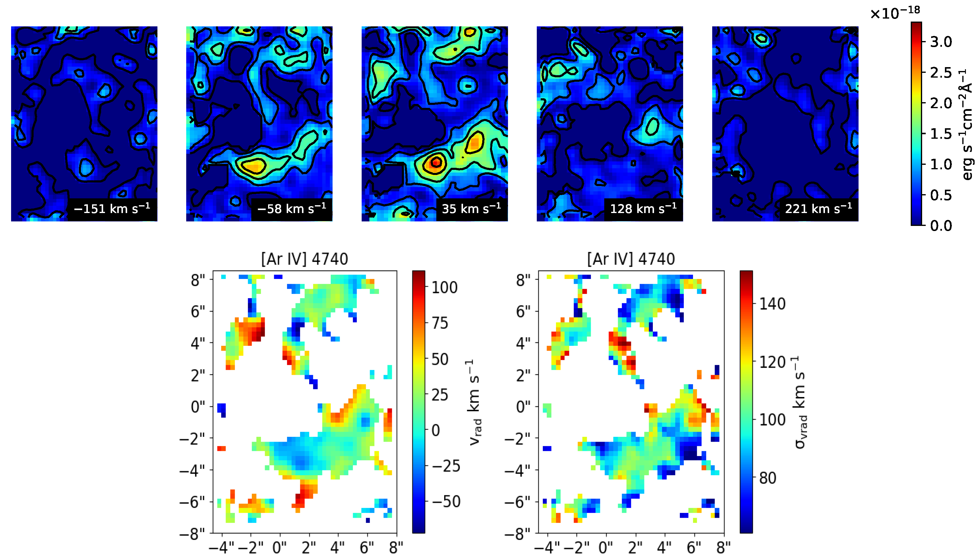
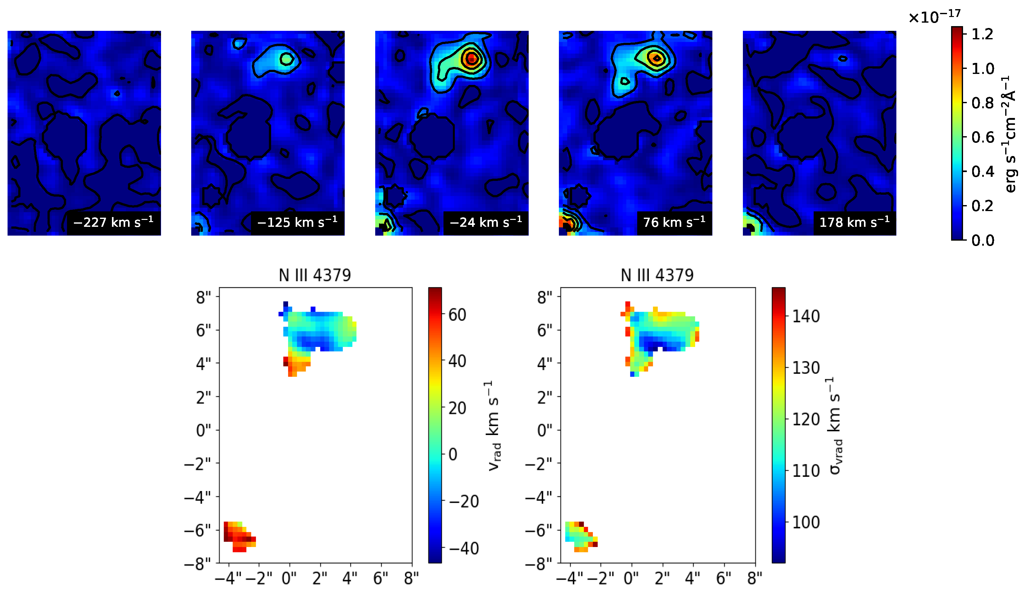
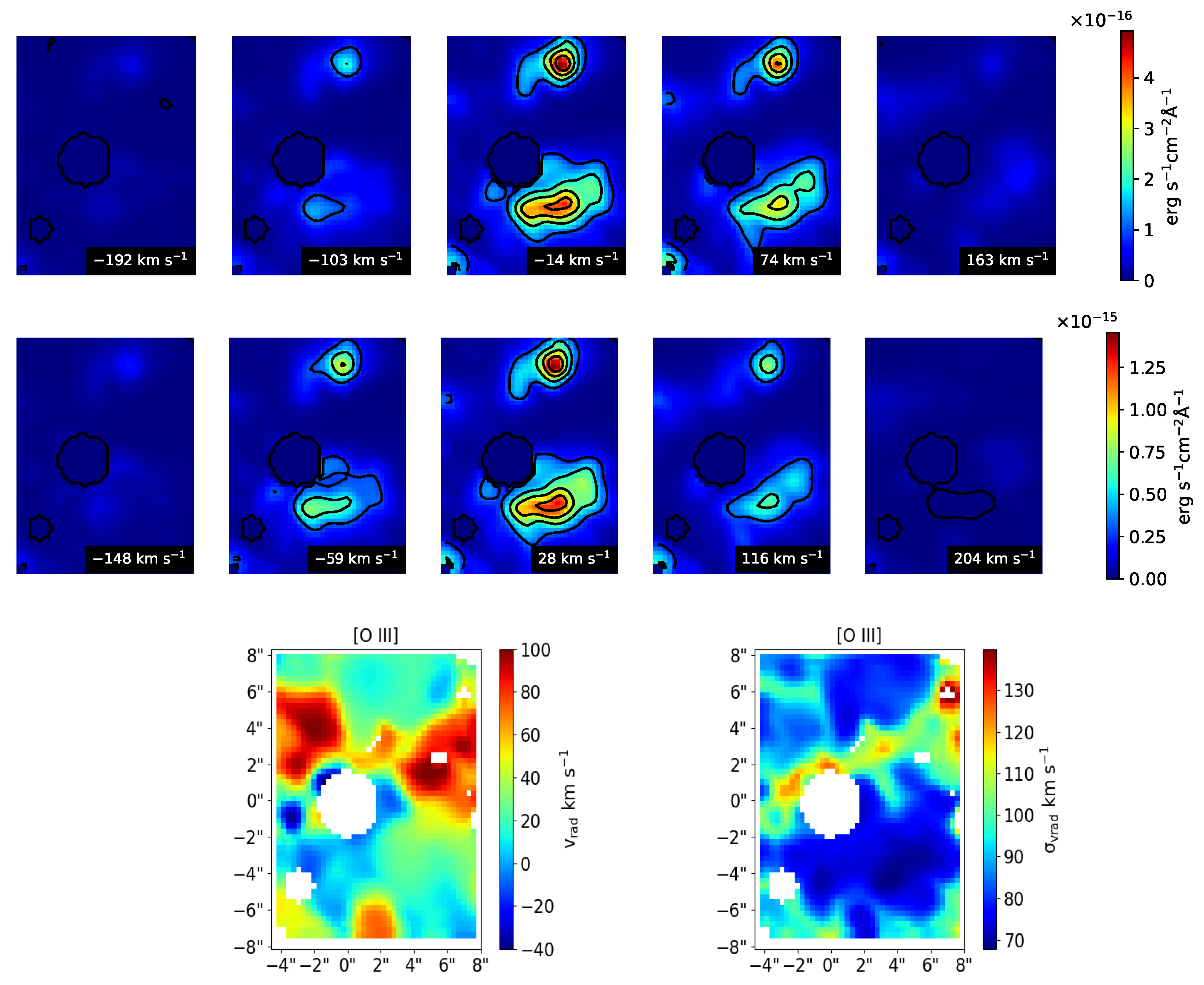
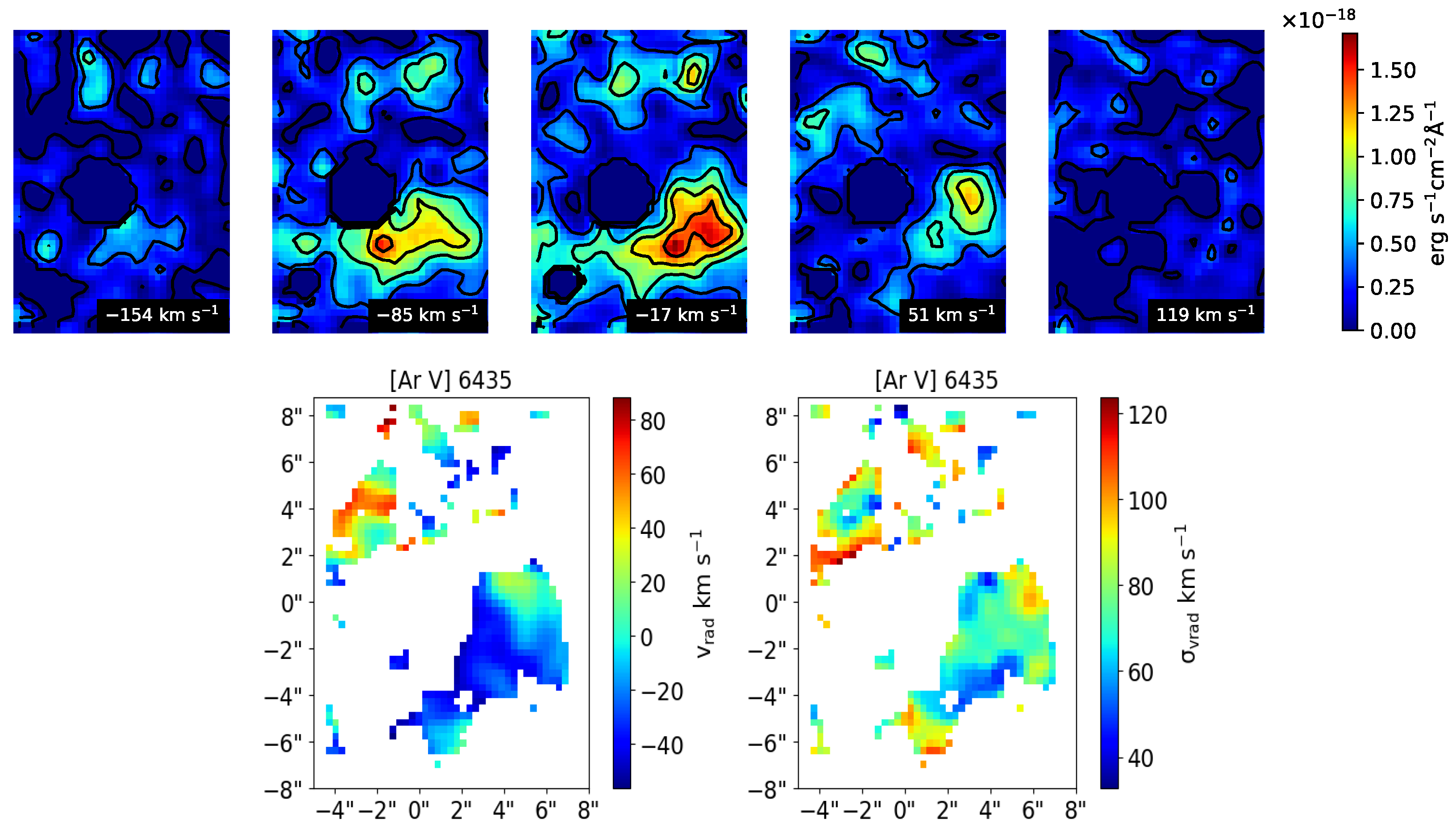
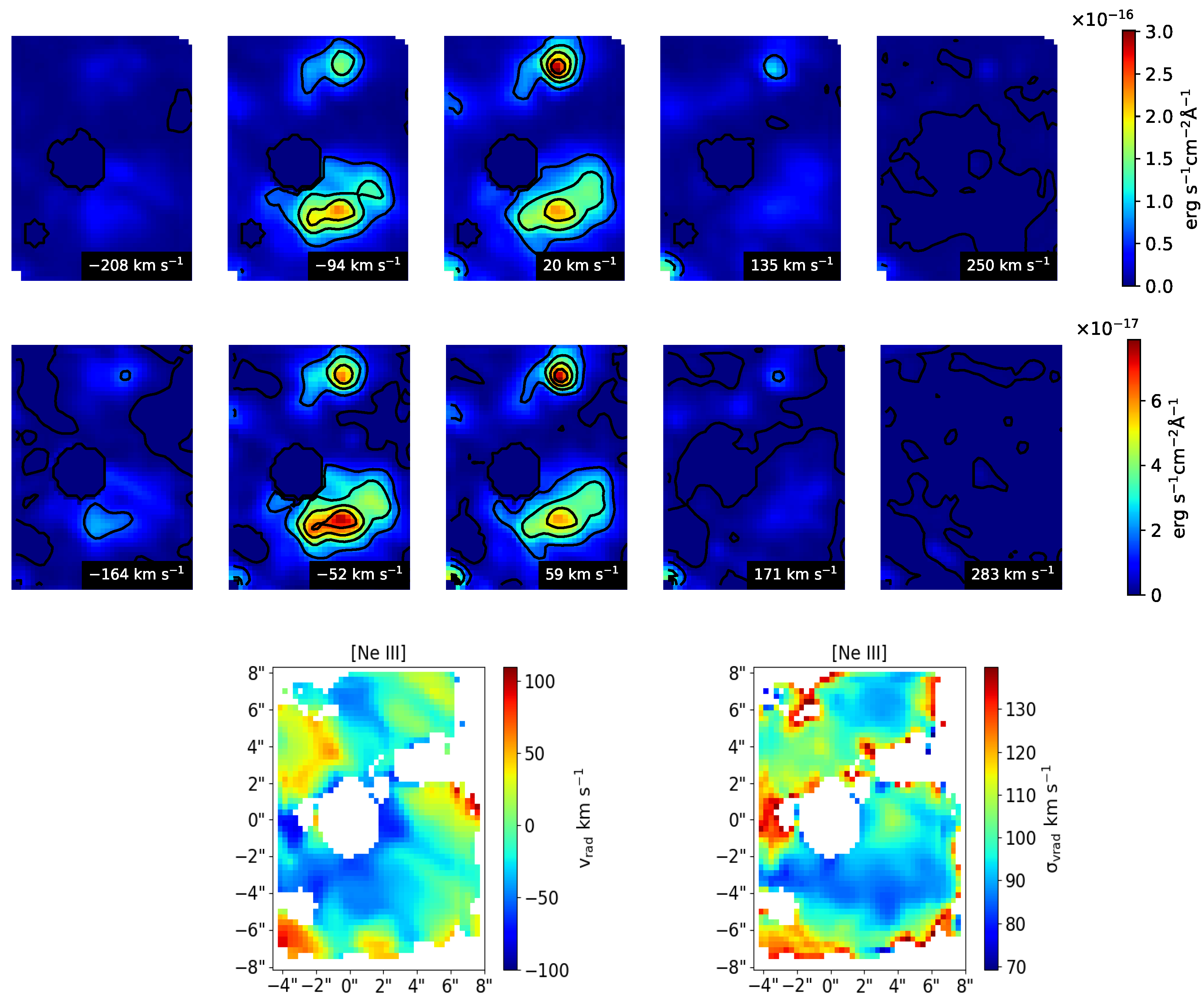
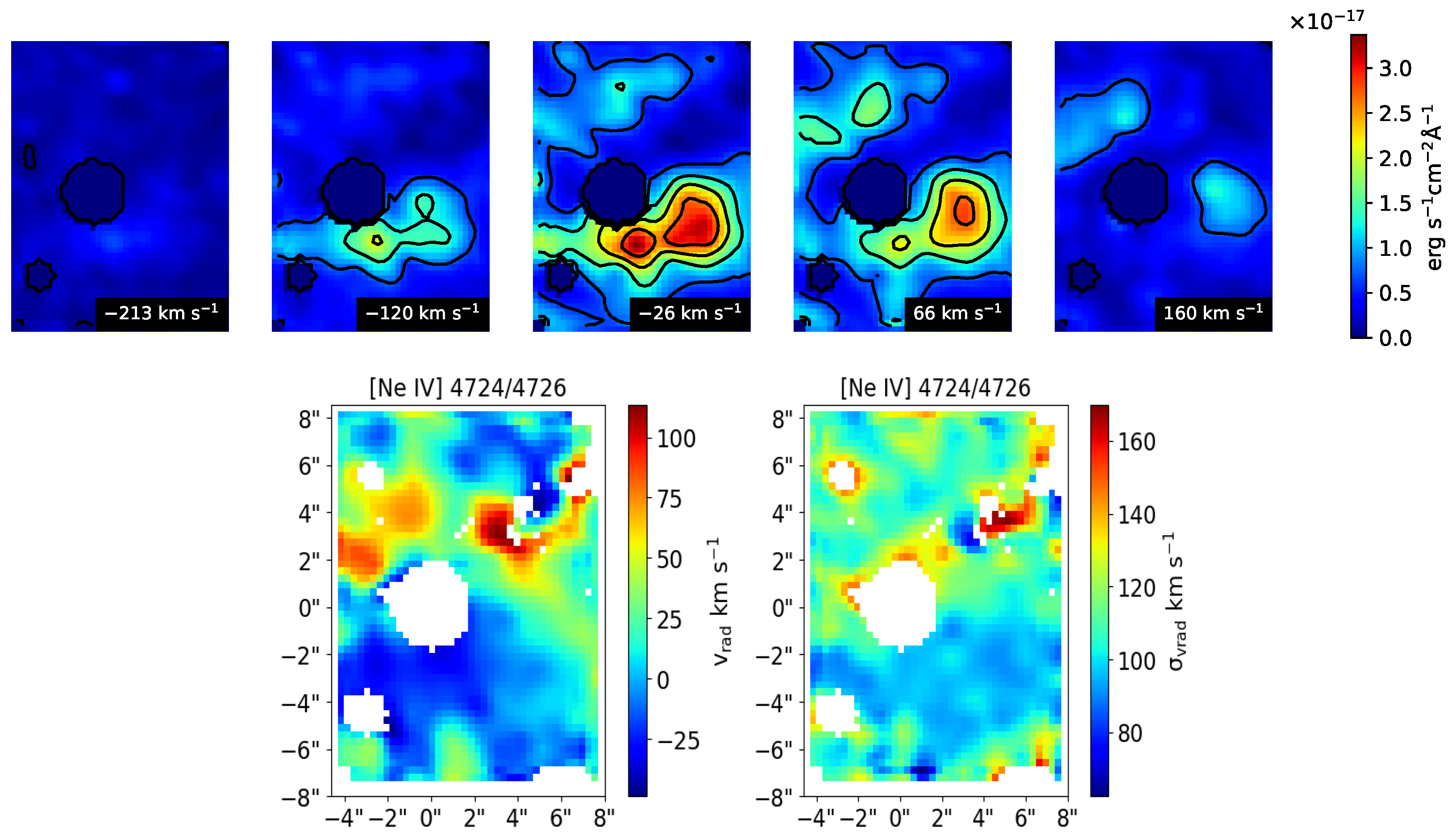
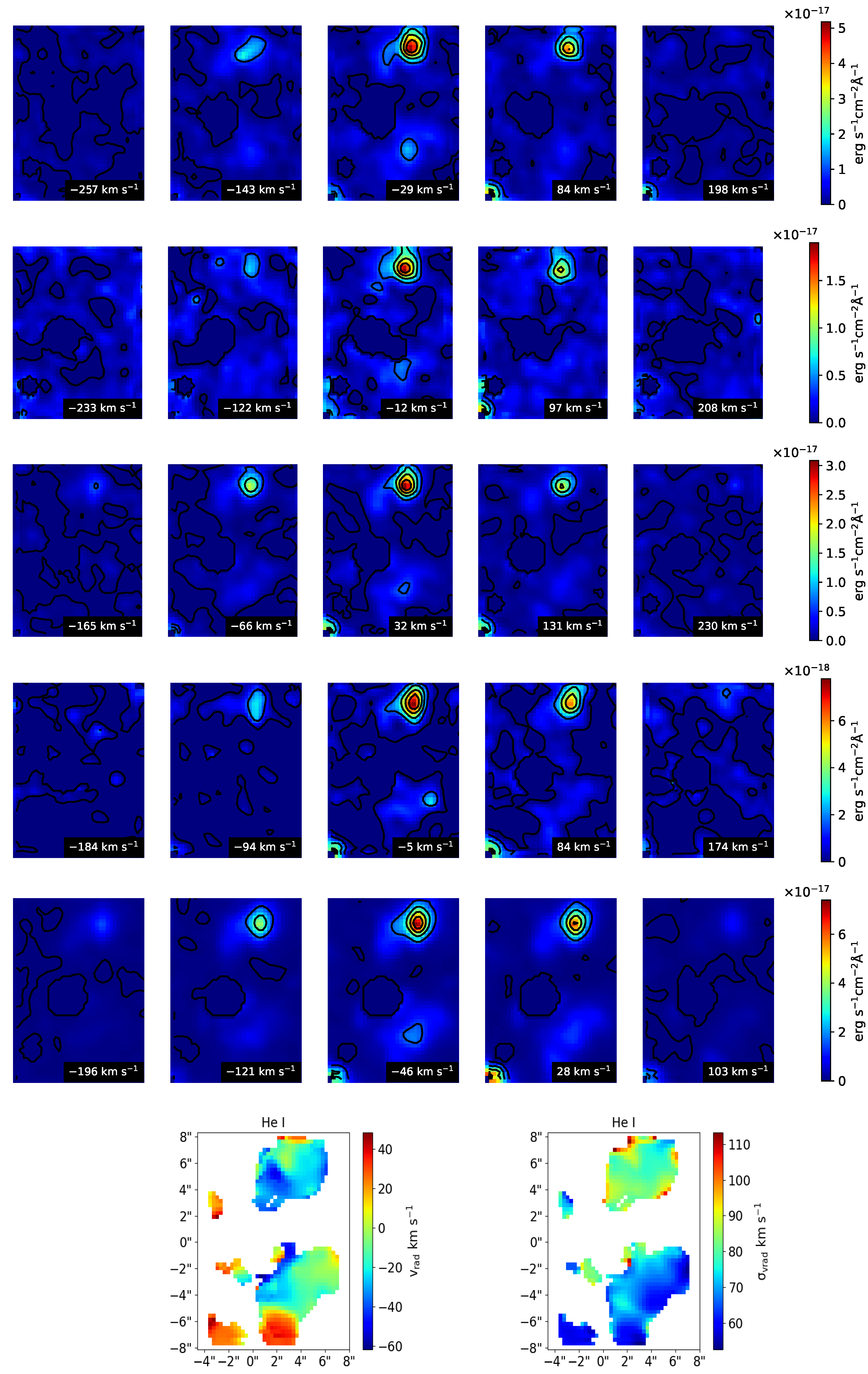
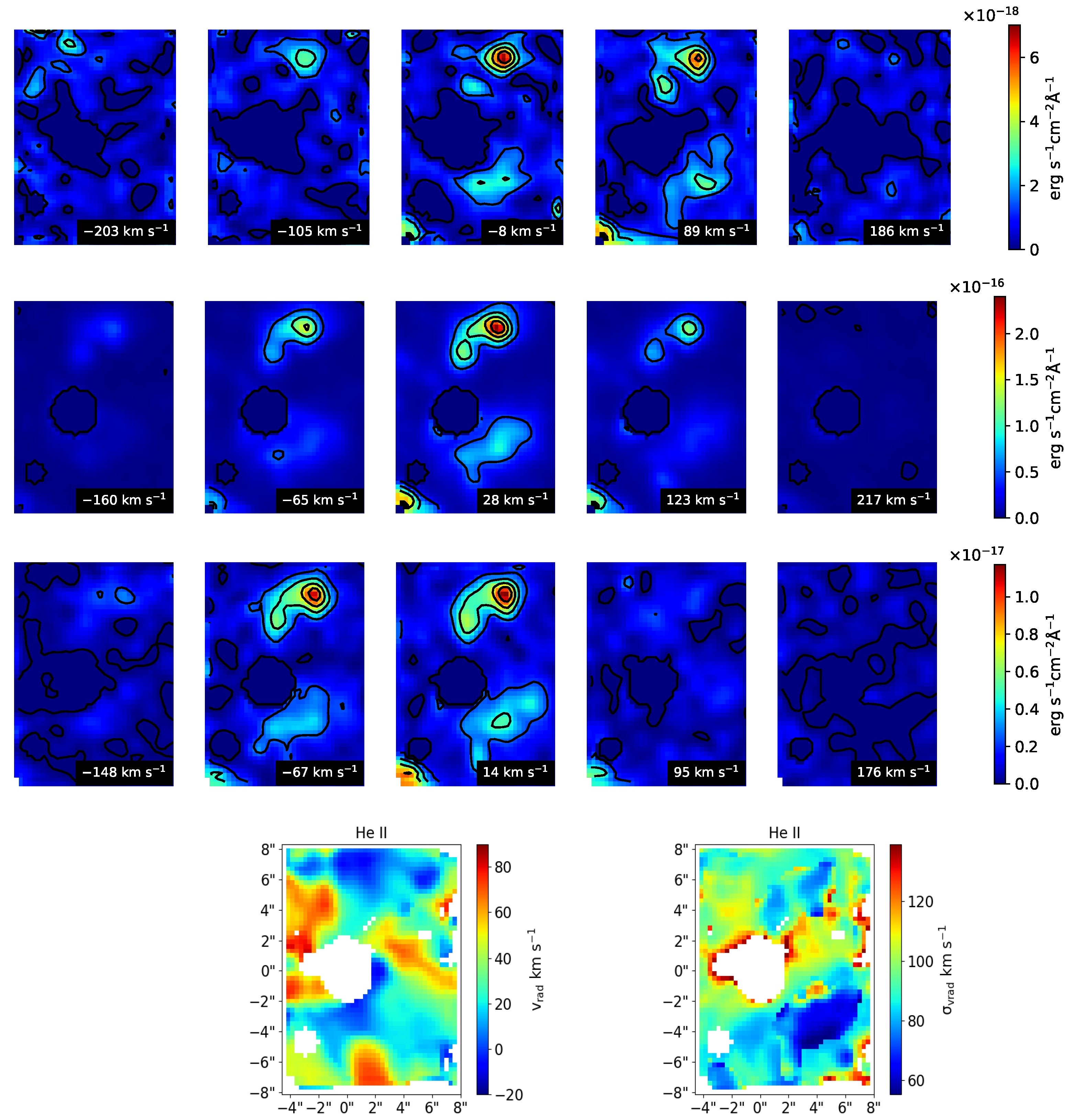
We produced kinematic maps (Figure 10 and Figure A1, Figure A2, Figure A3, Figure A4, Figure A5, Figure A6, Figure A7, Figure A8, Figure A9 and Figure A10 top panels) for each identified, un-blended line by plotting the measured flux density for each wavelength step and spaxel. To produce the velocity maps at the bottom panels of Figure 10 and Figure A1, Figure A2, Figure A3, Figure A4, Figure A5, Figure A6, Figure A7, Figure A8, Figure A9 and Figure A10, we fitted all lines of each ion species with signal-to-noise ratios (SNRs) greater than 3 simultaneously with the same velocity. As the velocity resolution changes with the wavelength, we set lower limits on the velocity dispersion of each line corresponding to the velocity resolution at those lines. The fitted mean velocities (relative to the laboratory wavelength) are shown in the left-hand plots of the bottom panels of each figure, while the velocity dispersions (in $\mathrm{km}{\mathrm{s}}^{-1}$) of the line with the highest velocity resolution (which is the reddest line) are shown on the right-hand side. All the contoured kinematic maps presented here are in linear scale. The mean radial velocities of a Gaussian fit for each ion species summed up for each knot are shown in

Table 2. Mean radial velocities of Gaussian fits for each ion species and knot.

	${\mathit{\mu }}_{\mathbf{vrad}}$ [$\mathbf{km}{\mathbf{s}}^{-1}$]
Ion	J1	J2	J3	J4
He I	31 ± 21	56 ± 33	−25 ± 22	−17 ± 26
He II	38 ± 18	48 ± 21	−2 ± 18	16 ± 19
C II	62 ± 32	38 ± 68	−2 ± 34	2 ± 83
[N II]	9 ± 6	23 ± 14	−26 ± 5	−19 ± 4
N III	41 ± 26	−68 ± 75	−14 ± 23	25 ± 86
O II	56 ± 37		12 ± 42	64 ± 93
[O III]	32 ± 17	68 ± 17	11 ± 17	17 ± 17
[Ar IV]	51 ± 98	53 ± 68	−7 ± 79	16 ± 74
[Ar V]	−15 ± 41	51 ± 49	−18 ± 41	−27 ± 27
[Ne III]	55 ± 23	25 ± 22	−11 ± 21	−30 ± 21
[Ne IV]	10 ± 37	44 ± 27	−7 ± 38	−11 ± 26
mean	34	34	−8	3
stddev	23	36	12	27

. We adopted the velocity uncertainties from the covariance matrix of the weighted least-squares fitting algorithm as error estimates. Note that the velocity dispersions stated in the table can arise either from actual turbulence or from differing velocities for the individual spaxels inside a knot. Additionally, the instrumental profile is wider in the blue region, leading to larger lower limits of the measured velocity dispersions compared to the lines in the red region.

The He I lines (see Figure 10) are quite weak but still very clearly detectable, mainly in knots J1 and J3 and less so in J4. For J2, barely any detection was possible. He I in J1 appears red-shifted by ≈30 $\mathrm{km}{\mathrm{s}}^{-1}$ while J3 and J4 are centred around −20 $\mathrm{km}{\mathrm{s}}^{-1}$. The velocity dispersions in J3 are greater compared to J1 and J4, indicating higher turbulence or multiple kinematic components in the line of sight.

The He II lines (see Figure A1) at 4542 Å and 5511 Å are very weak and subsequently quite noisy, while the 4686 Å line is reasonably strong and can be fitted across most of the FoV. The flux maps for the individual velocity steps of the 3 lines appear consistent. Knots J1, J2, and J4 appear to be slightly red-shifted, with the highest being J2 at ≈50 $\mathrm{km}{\mathrm{s}}^{-1}$, while J3 appears static. The lowest degree of turbulence is seen in J4, where the velocity dispersions are close to the lower limit set by the spectroscopic resolution. J2, however, shows velocity dispersions about twice as high. We note that the sharp edges of J4 in the velocity dispersion map are caused by the higher velocity resolution of the 5412 Å line compared to the strongest line at 4686 Å. As the 5412 Å line has a SNR below 3 in the areas surrounding J4, it was not included in the fits, explaining the sharp edges.

The C II 4267 Å line (Figure A2) is only detected in our maps in knots J1 and J3. While J1 is strongly red-shifted with velocities close to 60 $\mathrm{km}{\mathrm{s}}^{-1}$, J3 shows velocities around $0\pm 20$ $\mathrm{km}{\mathrm{s}}^{-1}$. J1 shows very little turbulence. The highest velocity dispersions with values exceeding 110 $\mathrm{km}{\mathrm{s}}^{-1}$ are seen between the higher-density sub-structures in J4.

The [N II] lines at 6548 Å and 6583 Å (Figure A3) are sampled at similar velocities. Maximum velocities with values of ≈30 $\mathrm{km}{\mathrm{s}}^{-1}$ are reached in J2, South–East of J4, as well as just East of the CS, and slightly less in J1. J3 is slightly blue-shifted with velocities of ≈−20 $\mathrm{km}{\mathrm{s}}^{-1}$ while the highest negative velocities with values of <−40 $\mathrm{km}{\mathrm{s}}^{-1}$ are found South and West of the CS. J4 is the least turbulent, with velocity dispersions of the Gaussian fits of ≈45 $\mathrm{km}{\mathrm{s}}^{-1}$, close to the lower limit set by the velocity resolution. J1, J2, J3 as well as the area South–East of J4 show more turbulent gas with velocity dispersions of ≈55–60 $\mathrm{km}{\mathrm{s}}^{-1}$. The highest turbulence—although the signal is quite faint—is found just South–East of the CS.

The weak N III line at 4379 Å (Figure A4) is clearly red-shifted at J1 with mean velocities of ≈40 $\mathrm{km}{\mathrm{s}}^{-1}$ and mildly blue-shifted at J3. The velocity dispersions between 120 and 140 $\mathrm{km}{\mathrm{s}}^{-1}$ are more than twice as high compared to the [N II] lines, although influenced by the wider instrumental profile. The turbulence in J3 shows a systematic trend to increase towards North.

The only O II line which is free of blends in our data is the 4649 Å line (Figure A5). The line is red-shifted for knots J1, J3, and J4, and not detected in J2. The highest velocities with values of up to ≈100 $\mathrm{km}{\mathrm{s}}^{-1}$ are found in the southern part of J4. Turbulence is moderate with an apparent sea-saw structure in knot J4 (values between 60 $\mathrm{km}{\mathrm{s}}^{-1}$ and 140 $\mathrm{km}{\mathrm{s}}^{-1}$) and relatively constant at ≈100 $\mathrm{km}{\mathrm{s}}^{-1}$ in J1 and J3.

The CELs of [O III] at 4363 Å, 4959 Å, and 5007 Å (Figure A6) show the highest velocities at ≈100 $\mathrm{km}{\mathrm{s}}^{-1}$ West for J2 and between J3 and J4. The knots themselves show moderate red-shifts with velocities of ≈30–50 $\mathrm{km}{\mathrm{s}}^{-1}$ in J1, ≈60–70 $\mathrm{km}{\mathrm{s}}^{-1}$ in J2, ≈10 $\mathrm{km}{\mathrm{s}}^{-1}$ in J3, and ≈20–30 $\mathrm{km}{\mathrm{s}}^{-1}$ in J4. Turbulence is relatively low with values around 70–80 $\mathrm{km}{\mathrm{s}}^{-1}$ in knots J3 and J4, ≈90 $\mathrm{km}{\mathrm{s}}^{-1}$ in J2, and 90–100 $\mathrm{km}{\mathrm{s}}^{-1}$ in J1. The strongest turbulence with values of 100–120 $\mathrm{km}{\mathrm{s}}^{-1}$ is found East and North of the CS as well as between J3 and J4, with the highest values of up to 140 $\mathrm{km}{\mathrm{s}}^{-1}$ West of J3.

The emission lines of [Ar IV] (4740 Å, Figure A7) and [Ar V] (6435 Å, Figure A8) are weak; however, some systematic movements can be seen. J1 and J2 for [Ar IV] 4740 Å are red-shifted with strongly varying mean velocities between 0 and $+100$ $\mathrm{km}{\mathrm{s}}^{-1}$, with the highest velocities actually between the knots. Velocities of J3 and J4 on the other hand are centred around ≈0 $\mathrm{km}{\mathrm{s}}^{-1}$. The strongest turbulence with velocity dispersions exceeding 140 $\mathrm{km}{\mathrm{s}}^{-1}$ is found just South of J3, while the knots show values of 60–130 $\mathrm{km}{\mathrm{s}}^{-1}$. [Ar V] 6435 Å exhibits different kinematics compared to [Ar IV]—while J2 is still strongly red-shifted with velocities up to ≈75 $\mathrm{km}{\mathrm{s}}^{-1}$, the other knots now appear blue-shifted with velocities between 0 and $-60$ $\mathrm{km}{\mathrm{s}}^{-1}$. J4 shows moderate turbulence of 50–100 $\mathrm{km}{\mathrm{s}}^{-1}$.

The kinematic morphologies of [Ne III] lines at 3869 Å and 3967 Å (see Figure A9) indicate that J1 is quite strong, and J2 and J3 are slightly red-shifted, while J4 is slightly blue-shifted. The fastest moving ions—moving at speeds of ≈100 $\mathrm{km}{\mathrm{s}}^{-1}$—can be found in J1 and North–West of J4. Knots J2–J4 exhibit moderate turbulence with velocity dispersions between 90 and 110 $\mathrm{km}{\mathrm{s}}^{-1}$, while J1 and the areas around the knots show larger values between 120 and 140 $\mathrm{km}{\mathrm{s}}^{-1}$.

The unresolved [Ne IV] 4724/4726 Å doublet (assumed remaining wavelength 4724.89 Å, Figure A10) shows that J2 is the most red-shifted with an average velocity of ≈50 $\mathrm{km}{\mathrm{s}}^{-1}$, J1 is slightly red-shifted, J3 shows velocities centred around 0 $\mathrm{km}{\mathrm{s}}^{-1}$ with strong red-shifts just South of it, and J4 is slightly blue-shifted. All knots show velocity dispersions around 100–110 $\mathrm{km}{\mathrm{s}}^{-1}$ while the area South of J3 shows values of up to 165 $\mathrm{km}{\mathrm{s}}^{-1}$. The direct comparison between the [Ne III] lines and the [Ne IV] 4724/4726 Å doublet shows various differences. The mean velocities in the knots differ quite strongly with J1, showing a much lower velocity for [Ne IV] (≈20 $\mathrm{km}{\mathrm{s}}^{-1}$) compared to [Ne III] (≈70 $\mathrm{km}{\mathrm{s}}^{-1}$). In contrast, ions just South of J2 and J3 show maximum velocities of ≈100 $\mathrm{km}{\mathrm{s}}^{-1}$ for [Ne IV], while both [Ne III] lines only show velocities of <50 $\mathrm{km}{\mathrm{s}}^{-1}$.

6. Discussion

6.1. Multiple Kinematic Components—Non-Uniform Velocity Distributions

Based on the work on A30 for the inner knot kinematic structure by [30], the knots possess different velocity components. The better resolved studies by [27,28] also reached similar findings, suggesting that the knots were not generated from a single episode of matter outflow but several—a rather complex process. Velocities derived in our study show a non-uniform velocity distribution among the knots, e.g., different mean velocities for emission lines originating from different ions of the same elements. While some of them may simply be due to low SNR, others appear to be more significant. Still, even these more significant systematics may have been caused by different effects. It is possible that a Gaussian is not an appropriate representation of the emission lines, leading to wrong fitted mean values. Other possible reasons are unidentified blends with lines from other atoms, data-reduction or wavelength-calibration problems/artifacts, or pixel-to-pixel correlations introduced by data (re-)binning. While our data show some evidence for this unexpected behaviour being real (supporting previous studies), only follow-up observations with higher spectral resolutions and higher SNRs can reveal the full picture.

The highest velocities are found between the knots, likely tracing low-density material, which has been accelerated by the stellar wind, while the higher-density material is shielded from the stellar wind, possibly by dust grains. Larger velocity dispersions of the Gaussian fits in these low-density regions fit this picture and can be explained with turbulence, while large velocity dispersions in the high-density regions may be due to either turbulence or multiple kinematic components in the same line of sight.

The knots themselves show multiple different velocity components with varying mean values and velocity dispersions. While knots J1 and J2 are consistently red-shifted (except for [Ar V] where J1 appears to be blue-shifted), J3 and J4 show red-shifted emission lines as well as blue-shifted ones. Notable outliers from the general velocity structures are the [N II] lines at 6548 Å and 6583 Å, which have the lowest velocity dispersions, and the [Ar V] line at 6435 Å, which is the only blue-shifted line in J1, red-shifted in J2, and the strongest blue-shifted line in J3 and J4.

As for the mean velocities for the individual knots stated in Table 2, it seems probable that the individual sub-knots visible in the HST image (Figure 1) have differing velocities, leading to several components within each integrated J complex. Follow-up observations with better spatial and velocity resolution are required to extend this study.

A new recurrent structure in the velocity maps, apart from the knots J1–4, is the circular area at 0″ < x < 3″, y < −5″, which, while not containing much flux itself, is consistently moving at mean velocities $2248;50$ $\mathrm{km}{\mathrm{s}}^{-1}$ higher compared to the surrounding area. The same structure can be identified in Figure 10, Figure A1, Figure A3, Figure A7, Figure A6, Figure A9 and Figure A10. Other new velocity structures moving with much higher velocities compared to their surrounding areas are the ones surrounding J2 and the area between J3 and J4, which are most prominent in Figure A6 and Figure A3, but also observable in Figure 10, Figure A1, Figure A7, Figure A9 and Figure A10. A small area just East of the CS at y values between 0″ and −2″ appears strongly red-shifted for He II while strongly blue-shifted for [O III] and [Ne III].

6.2. A30 and Its Massive Wolf–Rayet Counterparts

A30 hosts a central star of the Wolf–Rayet spectral type that has been categorised as a stage in transition between the spectral-type Wolf–Rayet star and PG 1159: [WC]-PG 1159 [31]. A number of massive Wolf–Rayet stars have been identified as either periodic or episodic dust makers [32]. It is believed that the wind collision region created by binary interaction often gives rise to strong compression and subsequent radiative cooling that leads to dust formation in these systems [33]. Examples of dust-making binary massive Wolf–Rayet systems that were detected with X-ray and radio emission include WR 140, WR 137, and WR 125 [34,35,36], where binary-driven shock-triggered dust formation was observed in both WR 140 and WR 137 [34,37]. Despite the long orbital period and periodic dust formation process of these Wolf–Rayet binary examples, physical phenomena, including dust formation, X-ray emission, and binary interaction, observed in these binary Wolf–Rayet cases make them a possible analogue for a better understanding of our A30 inner knot system characterised by its optical and X-ray signatures and suggested binary central star system.

7. Conclusions

We obtained integral field spectra of Abell 30’s inner knot system with a FoV of 12.3$″$× 16$″$. After data reduction, we integrated the IFU data cube slices into emission line flux maps for the detected spectral lines of He I and II, C II, [Ne III] and [Ne IV], [Ar IV] and [Ar V], O II and [O III], [N II] and N III.

ORLs of low-ionisation species predominantly populate the polar knots J1 and J3 while the CELs of high-ionisation species dominate the equatorial knots. Helium emission is strongest in J1 and J3, weaker in J4, and almost absent in J2. C II is strong in J1 and J3 and barely detectable in J2 and J4. [N II] is present in J1 and J3, and strongest in J4, where N III is barely visible. O II is strong in J1 and J3, absent in J2, and weak in J4, where strong but diffuse [O III] is seen. The CELs of Argon are strongest in J4 and only barely detected in the other knots. [Ne III] is present in all 4 knots while [Ne IV] is strong only in J4 with diffuse emission across most of the FoV.

The constructed temperature map based on the detected [O III] diagnostic lines shows cool cores (≈15,000 K) in the knots surrounded by hot outer regions exceeding 20,000 K, indicating possible shocks, shielding of the inner cores, or a combination of both.

For the velocity maps, we extracted IFU slices covering the detected spectral lines. Most observed lines in our data are red-shifted, with the strong exception of blue-shifted [Ar V] lines in J1, J3, and J4 (while J2, even though the signal is very weak, is red-shifted). J1 and J2 (where detected) are consistently red-shifted (with the exception of [Ar V] in J1) for all detected emission lines. J3 as well as J4 have mean radial velocities around 0 $\mathrm{km}{\mathrm{s}}^{-1}$. J3 shows mild to medium red-shifts for He II, C II, O II, [O III], and [Ne IV], while He I, [N II], [Ar IV], [Ar V], and [Ne III] are blue-shifted. For J4, He II, C II, N III, O II, [O III], and [Ne IV] are slightly red-shifted, while He I, [N II], [Ar V], [Ne III], and [Ne IV] are blue-shifted.

The differing velocity dispersions observed in all 4 knots (50 $\mathrm{km}{\mathrm{s}}^{-1}$$\le {\sigma }_{{\mathrm{v}}_{\mathrm{rad}}}\le 135$$\mathrm{km}{\mathrm{s}}^{-1}$) indicate a fast stellar wind, leading to turbulence that appears to affect different ions differently. Another possible interpretation could be different kinematic components along the same line of sight.

We have identified new recurrent structures in the velocity maps where the ions move up to ≈50 $\mathrm{km}{\mathrm{s}}^{-1}$ faster compared to the surrounding areas. The fact that these faster-moving ions are found between the knots can be interpreted as stellar wind accelerating the low-density regions, while the high-density regions are shielded. All these properties point at a rather complex ionisation structure and ejection history. We strongly encourage future IFU observations with higher spectral and spatial resolution.

References

1. Greenstein, J.L.; Minkowski, R. The central stars of planetary nebulae of low surface brightness. Astrophys. J. 1964, 140, 1601. [Google Scholar] [CrossRef]
2. Abell, G.O. Properties of some old planetary nebulae. Astrophys. J. 1966, 144, 259. [Google Scholar] [CrossRef]
3. Jacoby, G.H. Unusual structure in the planetary nebulae Abell 30 and Abell 78. Publ. Astron. Soc. Pac. 1979, 91, 754. [Google Scholar] [CrossRef]
4. Liu, X.-W.; Storey, P.J.; Barlow, M.J.; Danziger, I.J.; Cohen, M.; Bryce, M. NGC 6153: A Super-metal-rich planetary nebula? Mon. Not. R. Astron. Soc. 2000, 312, 585–628. [Google Scholar] [CrossRef]
5. Jacoby, G.H.; Ford, H.C. The hydrogen-depleted planetary nebulae Abell 30 and Abell 78. Astrophys. J. 1983, 266, 298. [Google Scholar] [CrossRef]
6. Jacoby, G.H.; Hillwig, T.C.; Jones, D. Abell 30—A binary central star among the born-again planetary nebulae. Mon. Not. R. Astron. Soc. Lett. 2020, 498, L114–L118. [Google Scholar] [CrossRef]
7. Harrington, J.P. Observations and models of H-deficient planetary nebulae. Astron. Soc. Pac. Conf. Ser. 1996, 96, 193. [Google Scholar]
8. Simpson, J.; Jones, D.; Wesson, R.; García-Rojas, J. Abundance analysis of the J4 equatorial knot of the born-again planetary nebula A30. Res. Notes Aas 2022, 6, 4. [Google Scholar] [CrossRef]
9. Toalá, J.A.; Jiménez-Hernández, P.; Rodríguez-González, J.B.; Estrada-Dorado, S.; Guerrero, M.A.; Gómez-González, V.M.; Ramos-Larios, G.; García-Hernández, D.A.; Todt, H. Carbon dust in the evolved born-again planetary nebulae a 30 and a 78. Mon. Not. R. Astron. Soc. 2021, 503, 1543–1556. [Google Scholar] [CrossRef]
10. Badenes, C.; Maoz, D.; Ciardullo, R. The progenitors and lifetimes of planetary nebulae. Astrophys. J. 2015, 804, L25. [Google Scholar] [CrossRef]
11. Kwok, S. The Origin and Evolution of Planetary Nebulae; Cambridge University Press: Cambridge, UK, 2000. [Google Scholar] [CrossRef]
12. Guerrero, M.A.; Manchado, A. The chemical abundances of the hydrogen-poor planetary nebulae A30 and A58. Astrophys. J. 1996, 472, 711–722. [Google Scholar] [CrossRef]
13. Herwig, F. Internal mixing and surface abundance of [WC]-CSPN. Astrophys. Space Sci. 2001, 275, 15–26. [Google Scholar] [CrossRef]
14. Toalá, J.A.; Guerrero, M.A.; Todt, H.; Hamann, W.-R.; Chu, Y.-H.; Gruendl, R.A.; Schönberner, D.; Oskinova, L.M.; Marquez-Lugo, R.A.; Fang, X.; et al. The born-again planetary nebula A78: An X-ray twin of A30. Astrophys. J. 2015, 799, 67. [Google Scholar] [CrossRef]
15. Iben, I.; Renzini, A. Asymptotic Giant Branch Evolution and beyond. Annu. Rev. Astron. Astrophys. 1983, 21, 271–342. [Google Scholar] [CrossRef]
16. Rodríguez-González, J.B.; Santamaría, E.; Toalá, J.A.; Guerrero, M.A.; Montoro-Molina, B.; Rubio, G.; Tafoya, D.; Chu, Y.-H.; Ramos-Larios, G.; Sabin, L. Common envelope evolution in born-again planetary nebulae—Shaping the H-deficient ejecta of a 30. Mon. Not. R. Astron. Soc. 2022, 514, 4794–4802. [Google Scholar] [CrossRef]
17. Borkowski, K.J.; Harrington, J.P.; Tsvetanov, Z.I. Interaction of a stellar wind with clumpy stellar ejecta in A30. Astrophys. J. 1995, 449, L143. [Google Scholar] [CrossRef]
18. Arribas, S.; Carter, D.; Cavaller, L.; del Burgo, C.; Edwards, R.; Fuentes, F.J.; Garcia, A.A.; Herreros, J.M.; Jones, L.R.; Mediavilla, E.; et al. INTEGRAL: A matrix optical fiber system for WYFFOS. In Optical Astronomical Instrumentation; Society of Photo-Optical Instrumentation Engineers (SPIE) Conference Series; SPIE: Bellingham, WA, USA, 1998; pp. 821–827. [Google Scholar]
19. Wesson, R.; Liu, X.-W.; Barlow, M.J. Physical conditions and abundances in Abell 30. Symp. Int. Astron. Union 2003, 209, 381–382. [Google Scholar] [CrossRef]
20. Sánchez, S.F. E3D, the Euro3D visualization tool I: Description of the program and its capabilities. Astron. Nachrichten 2004, 325, 167–170. [Google Scholar] [CrossRef]
21. Menezes, R.B.; Ricci, T.V.; Steiner, J.E.; da Silva, P.; Ferrari, F.; Borges, B.W. A treatment procedure for GMOs/ifu data cubes: Application to NGC 2835. Mon. Not. R. Astron. Soc. 2018, 483, 3700–3717. [Google Scholar] [CrossRef]
22. Guerrero, M.A.; Ruiz, N.; Hamann, W.-R.; Chu, Y.-H.; Todt, H.; Schönberner, D.; Oskinova, L.; Gruendl, R.A.; Steffen, M.; Blair, W.P.; et al. Rebirth of X-ray emission from the born-again planetary nebula A30. Astrophys. J. 2012, 755, 129. [Google Scholar] [CrossRef]
23. Harrington, J.P.; Feibelman, W.A. The remarkable ultraviolet spectrum of the planetary nebula Abell 30. Astrophys. J. 1984, 277, 716. [Google Scholar] [CrossRef]
24. Cohen, M.; Hudson, H.S.; O’Dell, S.L.; Stein, W.A. A study of the planetary nebulae Abell 30 and Abell 78. Mon. Not. R. Astron. Soc. 1977, 181, 233–245. [Google Scholar] [CrossRef]
25. Luridiana, V.; Morisset, C.; Shaw, R.A. PyNeb: Analysis of Emission Lines, Astrophysics Source Code Library, Record ascl:1304.021. 2013. Available online: https://ui.adsabs.harvard.edu/abs/2013ascl.soft04021L (accessed on 15 January 2024).
26. Cardelli, J.A.; Clayton, G.C.; Mathis, J.S. The Relationship between Infrared, Optical, and Ultraviolet Extinction. Astrophys. J. 1989, 345, 245–256. [Google Scholar] [CrossRef]
27. Fang, X.; Guerrero, M.A.; Marquez-Lugo, R.A.; Toalá, J.A.; Arthur, S.J.; Chu, Y.-H.; Blair, W.P.; Gruendl, R.A.; Hamann, W.-R.; Oskinova, L.M.; et al. Expansion of hydrogen-poor knots in the born-again planetary nebulae A30 and A78. Astrophys. J. 2014, 797, 100. [Google Scholar] [CrossRef]
28. Meaburn, J.; López, J.A. The dramatic kinematics of the hydrogen deficient planetary nebula Abell 30. Astrophys. J. Lett. 1996, 472, L45. [Google Scholar] [CrossRef]
29. Nyquist, H. Thermal agitation of electric charge in conductors. Phys. Rev. 1928, 32, 110–113. [Google Scholar] [CrossRef]
30. Jacoby, G.H.; Chu, Y.-H. Kinematics of Abell 30. Planet. Nebul. 1989, 131, 183. [Google Scholar] [CrossRef]
31. Werner, K.; Reindl, N.; Rauch, T.; El-Badry, K.; Bédard, A. The photospheres of the hottest fastest stars in the galaxy. Astron. Astrophys. 2024, 682, A42. [Google Scholar] [CrossRef]
32. Williams, P.M. Variable dust emission by WC Type Wolf–Rayet stars observed in the NEOWISE-R survey. Mon. Not. R. Astron. Soc. 2019, 488, 1282–1300. [Google Scholar] [CrossRef]
33. Hendrix, T.; Keppens, R.; van Marle, A.J.; Camps, P.; Baes, M.; Meliani, Z. Pinwheels in the sky, with dust: 3D modelling of the Wolf–Rayet 98a environment. Mon. Not. R. Astron. Soc. 2016, 460, 3975–3991. [Google Scholar] [CrossRef]
34. Lau, R.M.; Hankins, M.J.; Han, Y.; Argyriou, I.; Corcoran, M.F.; Eldridge, J.J.; Endo, I.; Fox, O.D.; Garcia Marin, M.; Gull, T.R.; et al. Nested dust shells around the wolf–rayet binary WR 140 observed with JWST. Nat. Astron. 2022, 6, 1308–1316. [Google Scholar] [CrossRef]
35. Lau, R.M.; Hankins, M.J.; Sanchez-Bermudez, J.; Thatte, D.; Soulain, A.; Cooper, R.A.; Sivaramakrishnan, A.; Corcoran, M.F.; Greenbaum, A.Z.; Gull, T.R.; et al. A first look with JWST aperture masking interferometry: Resolving circumstellar dust around the wolf–rayet binary WR 137 beyond the Rayleigh limit. Astrophys. J. 2024, 963, 127. [Google Scholar] [CrossRef]
36. Richardson, N.D.; Daly, A.R.; Williams, P.M.; Hill, G.M.; Shenavrin, V.I.; Endo, I.; Chené, A.-N.; Karnath, N.; Lau, R.M.; Moffat, A.F.; et al. The long-period spectroscopic orbit and dust creation in the wolf–rayet binary system WR 125. Astrophys. J. 2024, 969, 140. [Google Scholar] [CrossRef]
37. Zhekov, S.A. X-rays from the episodic dust maker WR 137. Mon. Not. R. Astron. Soc. 2015, 447, 2706–2713. [Google Scholar] [CrossRef]
38. Robitaille, T.P. et al. [Astropy Collaboration] Astropy: A community Python package for astronomy. Astron. Astrophys. 2013, 558, A33. [Google Scholar]
39. Price-Whelan, A.M. [Astropy Collaboration]. The Astropy Project: Building an Open-science Project and Status of the v2.0 Core Package. Astron. J. 2018, 156, 123. [Google Scholar]
40. Price-Whelan, A.M. et al. [Astropy Collaboration] The Astropy Project: Sustaining and Growing a Community-oriented Open-source Project and the Latest Major Release (v5.0) of the Core Package. Astrophys. J. 2022, 935, 167. [Google Scholar]
Figure 1. Left panel: Gas clump identification of knots J1–J4 from the outlined regions in white overlaid on the [O III] optical image of the central inner region of A30, adopted from the Hubble Space Telescope WFPC2 [17]. North is up and East is to the left. Right panel: An integrated flux map of [O III] 5007 Å as an example of the IFU sampled area with a FoV of 12.3″× 16″. Note that the central star (CS) and its surrounding region were masked.
Galaxies 14 00011 g001
Figure 2. Integrated flux maps of spectral lines of He I (left) and He II (right). Note the masked central star and background star.
Galaxies 14 00011 g002
Figure 3. The same as Figure 2, but for C II 4267 Å.
Galaxies 14 00011 g003
Figure 4. The same as Figure 2 but for [N II] 6548 Å + 6583 Å (left) and N III 4379 Å (right).
Galaxies 14 00011 g004
Figure 5. The same as Figure 2 but for (from left to right) O II 4649 Å, [O III] 4363 Å, [O III] 4959 Å + [O III] 5007 Å. Note that the 4363 Å line and the sum of 4959 Å and 5007 Å are shown separately as they carry the electron temperature information (see below).
Galaxies 14 00011 g005
Figure 6. The same as Figure 2 but for [Ar IV] 4740 Å (left) and [Ar V] 6435 Å (right).
Galaxies 14 00011 g006
Figure 7. The same as Figure 2 but for [Ne III] 3869 Å + 3967 Å (left) and [Ne IV] doublet 4724/4726 Å (right).
Galaxies 14 00011 g007
Figure 8. Integrated flux maps of top: ORLs of left: 3 lowest ionisation species He I (red), C II (green), and O II (blue); right: 3 highest ionisation species O II (red), He II (green), and N III (blue). Bottom: CELs of left: 3 lowest ionisation species [N II] (red), [O III] (green), and [Ne III] (blue); right: 3 highest ionisation species (except for Ar which is very weak and noisy) [O III] (red), [Ne III] (green), and [Ne IV] (blue). Note that for each species multiple line fluxes were summed up and all fluxes were scaled to a maximum of 1.
Galaxies 14 00011 g008
Figure 9. (Left) [O III] ratio map λ 5007/4363 Å. (Right) Electron temperature map derived from [O III] ratio map on the left.
Galaxies 14 00011 g009
Figure 10. Kinematic structure of He I (from top to bottom) 3889 Å, 4026 Å, 4472 Å, 4922 Å, and 5876 Å. The first 5 rows show the flux density values of the individual spaxels at velocities calculated with respect to the remaining wavelengths of the individual lines. The bottom row shows the mean velocities for each spaxel (left) as well as the velocity dispersions (in km s 1 , right).
Galaxies 14 00011 g010