Abstract
We develop predictive models for OH maser occurrence in Galactic star-forming regions by integrating dense-clump physical properties from the APEX Telescope Large Area Survey of the Galaxy (ATLASGAL) and Herschel Infrared Galactic Plane Survey (Hi-GAL) 360° catalogs with maser detections and non-detections compiled in the MaserDB.net database. We compare two predictive modeling approaches for Galactic OH maser incidence: a Generalized Linear Model (GLM; logistic regression) and a compact Keras-based binary neural network (BNN). For the 1665/1667 MHz lines, both models achieve recall of 90% with a precision of approximately 50%, while for the excited-state 6031/6035 MHz lines, precision reaches roughly 20% at the same recall. We found no statistically significant difference between the BNN and GLM in out-of-sample performance. This implies that maser occurrence may be expressed as a monotonic trend without requiring nonlinear interactions. Across different catalogs and transition lines, luminosity, luminosity-to-mass ratio (), dust temperature, and column, surface, and volume densities are the most influential features for maser prediction. These variables support a physical picture in which radiative pumping favors warm, luminous, and compact clump environments. We provide an accessible online tool that allows users to predict the likelihood of OH maser emission toward ATLASGAL or Hi-GAL sources based on coordinate lists.
1. Introduction
Astrophysical masers from molecules such as OH are powerful diagnostics of the physical conditions and evolutionary stages in massive star-forming regions. Ground-state OH masers at 18 cm (1612/1665/1667/1720 MHz) and excited-state OH lines (e.g., 6035 MHz) are typically radiatively pumped in warm, dense gas near ultracompact H II regions [1,2]. Large blind surveys such as THOR and SPLASH have dramatically expanded the census of OH masers [3,4], while ATLASGAL and Hi-GAL provide homogeneous clump catalogs with distances, luminosities, masses, and dust temperatures [5,6,7]. OH maser incidence is low in the general clump population (a few percent) and OH-maser-bearing clumps tend to be more luminous and warmer [8,9,10].
Predicting whether a given dense clump hosts a maser from its bulk properties is valuable both scientifically (to understand drivers such as luminosity-to-mass ratio and dust temperature) and operationally (to search for new maser sources). Machine-learning approaches have become powerful tools for analysis of large datasets and uncovering complex relationships in astronomy and other fields [11,12,13,14,15]. Prior studies have successfully used generalized linear models (GLMs; logistic regression) for maser prediction and related tasks (e.g., [9,16]). GLMs provide interpretable linear effects on the log-odds of maser occurrence, facilitating physical insight. Neural networks can capture nonlinear interactions among features and may improve recall and discrimination on complex tabular data, albeit with reduced interpretability [17,18]. However, the question of which model family is better for maser prediction is still open.
MaserDB.net is a consolidated database of Galactic maser observations with an emphasis on star-forming regions [19,20]. It aggregates targeted and blind-survey measurements across multiple molecular species and transitions, recording specific details of each observation. The MaserDB.net database uses spatial grouping of observations with the DBSCAN [21] algorithm, allowing the study of multi-epoch observations and cross-matching with clump catalogs. The service provides web query pages and CSV exports suitable for programmatic workflows (as used in this work). Both detections and non-detections are included in the database, enabling supervised learning with a substantial number of negatives. For OH specifically, MaserDB.net covers the ground-state 18 cm lines (1612/1665/1667/1720 MHz) as well as the excited-state transitions (6031, 6035 MHz, and others), linking large surveys such as THOR and SPLASH with numerous targeted studies.
In this work, we combine MaserDB.net labels (detections and non-detections) with clump properties from ATLASGAL and Hi-GAL catalogs to train and evaluate two families of maser predictors: (i) a GLM (logistic regression with p-based stepwise selection) and (ii) a compact binary neural network (BNN). We test whether a compact neural network outperforms a GLM for maser prediction. This approach is physically motivated, as maser emission is intrinsically tied to the properties of host molecular clumps. The physical parameters of dense clumps, such as luminosity, luminosity-to-mass ratio (L/M), dust temperature, and various density metrics, serve as direct proxies for the conditions required for maser pumping mechanisms to operate. Indeed, maser-bearing clumps are observationally confirmed [6,9,22,23,24] to be denser, more luminous, and more evolved, with both L/M and dust temperature acting as key diagnostics of evolutionary stage [6]. Furthermore, it was previously reported that maser presence is associated with clumps of high masses, radii, and flux densities [25,26]. By modeling these parameters, our algorithms effectively learn to identify the specific astrophysical environments conducive to maser activity.
The primary goal of this work is to develop a predictive tool to aid in the discovery of new masers. We define our evaluation metrics in terms of astronomical survey standards: Recall corresponds to completeness (the fraction of true masers correctly identified), while Precision corresponds to detection rates (the fraction of predicted candidates that are true masers). For discovery science, the strategic trade-off is clear: a candidate list containing some false positives (lower detection rate) is scientifically preferable to one that omits true masers (lower completeness), as each missed source is a lost opportunity for discovery. Consequently, our models are evaluated in a high-recall regime, specifically targeting the recovery of at least 90% of known masers.
2. Methods
2.1. Catalogs of Clump Physical Parameters and Maser Detections
Dense clump properties are drawn from three widely used catalogs, chosen to span complementary wavelength coverage and sky footprints, and to enable cross-checks of parameter systematics.
The APEX Telescope Large Area Survey of the Galaxy (ATLASGAL) provides 870 m continuum maps of the inner Milky Way and a compact source catalog of dense clumps [27]. The ATLASGAL 2018 catalog release [5] (hereafter AG) provides distances estimation and a suite of derived physical properties—including luminosity (L), mass (M), luminosity-to-mass ratio (), dust temperature (), and column density—for thousands of dense clumps in the inner Galaxy. The 870 m selection favors high column density, actively star-forming clumps and provides a uniform, single-band coverage for dense gas structures in the region , .
The updated 2022 release [6] (hereafter AG2) refines distances and physical parameters and emphasizes evolutionary trends across the high-mass clump population. In our analysis, we consider the AG and AG2 catalogs as complementary and partially overlapping datasets. This approach allows us to evaluate the sensitivity of model performance to catalog-specific choices—such as changes in distance estimates, SED fitting methods, and improved physical parameters—and to test the robustness of predictions against major catalog revisions and systematic updates in input clump properties.
The Herschel Infrared Galactic Plane Survey (Hi-GAL) mapped the Galactic plane in five far-infrared bands (70–500 m). The Hi-GAL 360 compact source catalog [28] (hereafter HG3) provides all-sky-plane coverage with SED-fitted clump properties (including , L, and M) at angular resolutions that vary by band. Compared to a single-band submillimeter catalog, far-IR SED fitting improves temperature estimates and extends sensitivity to somewhat colder and lower-mass clumps, and crucially covers the outer Galaxy beyond the ATLASGAL footprint.
The AG and AG2 catalogs deliver uniform 870 m coverage optimized for identifying high column density structures in the inner Galaxy, whereas the HG3 catalog provides comprehensive Galactic plane coverage with multi-band SED fitting, yielding robust constraints on dust temperature (). By training and evaluating maser detection models on these distinct catalogs, we assess and mitigate catalog-specific biases.
Maser labels (detections and non-detections) are sourced from the MaserDB.net database. For the present work we focus on OH masers associated with star formation, drawing on the main ground-state OH lines (1612/1665/1667/1720 MHz) and the excited-state (6031 and 6035 MHz) transitions. Representative large contributions include THOR and SPLASH for OH [3,4], complemented by numerous targeted studies (more than 60 papers https://MaserDB.net/list.pl, accessed on 20 October 2025). The database contains information about maser detections as well as non-detections. In the case of blind surveys, the database includes information about non-detections as well, but limited to the sources with detections in at least one frequency band. The specific transitions used for model training in this paper are 1612, 1665, 1667, and 1720 MHz (ground state), and 6031 and 6035 MHz (excited state). We exclude rarer OH excited-state transitions (e.g., 4765 MHz) from quantitative modeling in this work due to very small sample sizes (fewer than 40 sources associated with AG/HG3 catalogs) and heterogeneous selection, which would undermine statistical reliability.
The MaserDB.net database contains information about maser non-detections, which is crucial for model learning. However, the number of non-detections is still not enough to construct reliable predictive models. For example, for the 1665 MHz transition, the number of non-detections is only 27% of the number of detections. The reason for this is that targeted surveys usually aim at the known star-forming regions from blind surveys, resulting in low numbers of non-detections. To construct reliable negative labels, we consider using blind surveys with uniform coverage and well-defined sensitivity limits, allowing us to treat the absence of a cataloged maser as a non-detection within the survey footprint. For OH ground-state lines (18 cm), we consider THOR (northern inner plane: , , [3]) and SPLASH (southern plane: , , [4,29]) surveys. The typical rms noise level in the THOR (VLA) survey is 10 mJy , and a 2 threshold (20 mJy ) was used for signal identification. Since masers are generally unresolved, the minimum detected flux density in THOR can be taken as 0.02 Jy. In the SPLASH survey, the initial observations with the 64-m Parkes telescope had a typical rms of 65 mJy and a 5 detection threshold of 0.325 Jy. Therefore, in terms of completeness, THOR is significantly deeper. From the MaserDB.net portal we found that only three sources among 589 objects detected at 1665 MHz have maximum flux density lower than 0.025 Jy, but number of known maser sources below SPLASH detection threshold (<0.325 Jy) is 129 (23%) for 1665 MHz maser sources. Authors [3] concluded that the THOR maser data are complete at around the level of 0.25 Jy . Thus we used THOR data for training non-detection in this work, but SPLASH data is only used for training the maser detections. The primary reason of false negatives in THOR data is the source variability.
We assign a clump as a non-detection if no maser is cataloged within (∼2.5 times the typical ATLASGAL beam and comparable to positional uncertainties in cross-matching). This conservative radius reduces false negatives from masers cataloged with positional uncertainties and in complex regions. As the surveys do not overlap, they provide well-defined non-detection labels from the northern and southern Galactic planes.
2.2. Generalized Linear Model (GLM)
We use logistic regression [18] with standardized clump properties (, , , , etc.) as predictors. The model specifies
where is the probability of maser presence and are coefficients estimated by maximizing the Bernoulli likelihood. Each represents the change in log-odds per unit change in feature , enabling direct physical interpretation [9,16].
We use stepwise refinement guided by p-values (forward–backward logistic regression): at each step we remove variables with p-value and retain those with the strongest evidence (). We also tested an AIC-driven variant (Akaike Information Criterion); across lines and surveys it provides only marginal improvements in accuracy () while selecting more variables than the p-value method, but always consistent with significant parameters selected by the p-based method. Given the negligible gain and increased complexity, we adopt the p-value method for all comparisons. Prior to stepwise selection, we remove features that are nearly constant, exact duplicates, or highly correlated (). We focus on main effects for clarity. To make predictions, we set a threshold on to reach the desired recall, and evaluate performance using precision, recall, and partial AUC–PR (see Section 2.4).
As our training data reveal class imbalance, the class_weight parameter of scikit-learn’s LogisticRegression routine was used. This parameter is used to handle imbalanced datasets by assigning different weights to the samples of different classes during model training. This helps prevent the model from being biased towards the majority class.
2.3. Neural Network for Binary Classification
We implement a compact feed-forward binary neural network (BNN) using the high-level Keras API to test whether a model capable of learning nonlinear feature interactions could outperform the linear GLM. The architecture comprises two hidden layers (32 and 16 ReLU units) with batch normalization and dropout (0.2) for regularization, followed by a sigmoid output layer yielding maser probability [17,30].
To address class imbalance, we apply inverse-frequency class weights in the binary cross-entropy loss. We optimize with Adam (75 epochs, batch size 128) and use early stopping (patience 30) when validating. For k-fold cross-validation, the model is re-initialized in each fold. The BNN can capture nonlinear feature interactions at the cost of reduced interpretability relative to the GLM.
2.4. Metrics and Cross-Validation
Given severe class imbalance (maser detections comprise a few percent of clumps), accuracy is misleadingly high and uninformative. We therefore evaluate models via precision (fraction of predicted masers that are true), recall (fraction of true masers recovered), and partial AUC under the precision–recall curve for :
For completeness we also report the F1 score, defined as the harmonic mean of precision and recall,
This study focuses evaluation on the high-recall regime to cover significant fracion of maser sources. We target and compare models at matched recall using precision. We set the BNN threshold to reach and choose the GLM threshold to match that recall per survey and transition. This allows to compare the GLM and BNN models using precision at the same recall level. We also examine a high-precision regime to increase the detection rates with a target recall of ∼50%.
We validate the models using two similar protocols:
- Single split: Random 70/30 train/validation partition (fixed seed for reproducibility).
- Stratified 5-fold CV: The dataset is partitioned into five folds preserving class proportions; each fold serves once as validation while the model trains on the remaining four. We report mean and standard deviation of metrics across folds.
Both protocols apply equally to GLM and BNN. Cross-validation guards against overfitting, particularly for the BNN, where excessive epochs can yield high training performance but poor generalization.
We quantify the predictive contribution for specific features with drop-column LOCO (Leave-One-Covariate-Out; [31]) importance at high recall: we refit the GLM without particular predictor and evaluate on held-out data, computing the drop in partial AUC–PR restricted to ,
Positive values indicate that removing the feature harms performance; negative values indicate that the group is detrimental (or redundant) on held-out data. We note that only high-recall (R > 0.7) AUC-PR values are considered to measure the importance of the features.
3. Results
3.1. Metrics
Table 1 summarizes the number of detections and total sources observed for each survey and OH transition, representing the sample sizes used to train and evaluate our models. The large number of non-detections in the sample is due to non-detections of masers toward ATLASGAL/Hi-GAL sources within the coverage of the THOR blind survey. Primarily due to maser variability, non-detections may contain false negatives. We estimate the number of false negatives by counting the non-detections at 1665 MHz in the THOR survey that simultaneously have detections at 1665 MHz in other targeted surveys. We found 35 such cases, which is ≃6% of the total number of non-detections in the THOR survey at 1665 MHz (582 objects).

Table 1.
Detections and observed sources by frequency and survey.
Table 2 summarizes precision (P), recall (R), and partial AUC-PR () across OH transitions and surveys (AG, AG2, HG3) for three evaluation protocols: no-split case (full training set), single split case (30% validation set), and stratified 5-fold CV case (mean ± standard deviation). In Figure 1 we also present visualization of precision (P), recall (R), and F1 metrics in two regimes: high-recall (a) and high-precision (b). These two regimes display model performance in two task-dependent cases: when users require high precision (maser detection rates) or high recall (maser completeness). In the high-recall regime the detection threshold was set to obtain a recall of ∼90%. In the high-precision regime the threshold was set to obtain a recall of ∼50%.
Table 2.
Summary metrics by mode.
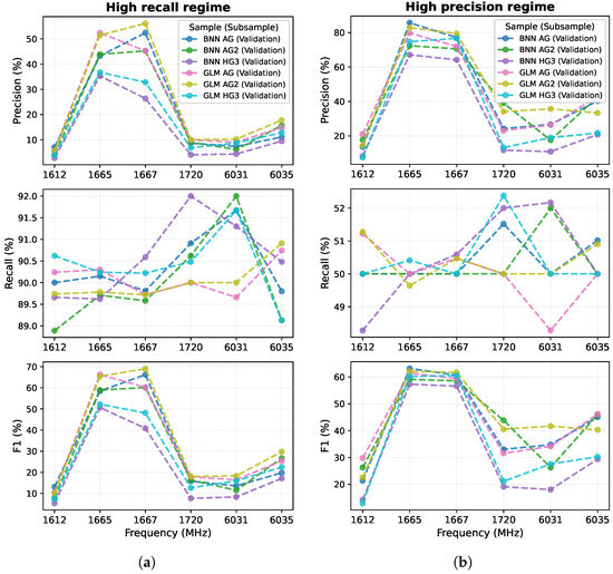
Figure 1.
Metrics (precision, recall and F1) of different models as a function of OH maser transition frequency. Left panels (a) correspond to high-recall regime, while right panels (b) correspond to high-precision regime.
In the no-split case, the BNN appears 8–13% better in precision and partial AUC–PR, but this advantage disappears on held-out data and across folds: GLM and BNN perform comparably, with fold-to-fold variability exceeding any consistent difference. At high recall, they are statistically equivalent; the GLM additionally offers interpretability.
As seen in Table 2, the 1665 and 1667 MHz transitions are consistently the easiest to predict: across AG, AG2, and HG3 they achieve the highest precision and partial AUC–PR under both single-split and 5-fold validation. The 1612 and 1720 MHz lines perform markedly worse, and the excited-state 6031/6035 MHz transitions generally trail the main lines, reflecting smaller samples and greater heterogeneity.
3.2. Precision-Recall Curves
The tradeoff between precision and recall is not fully captured by summary tables like Table 2, so we present the full precision–recall (PR) curves for our models. Figure 2 displays PR curves for the studied models on different OH transitions. The PR curves were constructed using the validation (unseen) data. We use a 50/50 train/validation split to reduce variance in the PR curves. This differs from the 70/30 split in Table 2, but performance trends are similar. Each panel compares results from the three surveys (AG, AG2, HG3) and modeling approaches (BNN, GLM, GLMsw); the curve achieving the highest partial AUC–PR in the high-recall region () is highlighted in red.
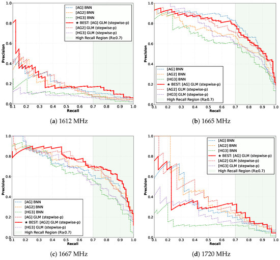
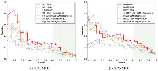
Figure 2.
Precision–recall curves for OH maser prediction across all frequencies. Subfigures show different OH maser transitions. Each subfigure shows models from different surveys (AG, AG2, HG3) and training methods (BNN, GLM) for a specific OH transition. The curve with the highest partial AUC–PR in the high-recall region () is highlighted. The green shaded region indicates the evaluation range. Different panels (a–f) represent different OH maser transitions.
Pairwise comparisons (Kolmogorov–Smirnov test) typically yield , and practical differences are small. The PR curves confirm that GLM and BNN trade off precision and recall similarly at operational thresholds. AG and AG2 perform slightly better than HG3, matching Table 2.
3.3. Feature Importance
From Table 2 we can see that the difference between the GLMsw (stepwise refinement) and the GLM (all features) is not statistically significant; within the standard deviation they are the same when comparing the fold metrics. However, the simplicity of the GLMsw is higher due to the smaller number of features, thus it is easier to use for physical interpretation. We summarize the selected features for the GLMsw in Table 3. The values in Table 3 are scaled GLM coefficients. The standard deviation was calculated by dividing the full dataset into five training/validation folds and averaging the results across these folds. We note that feature selection is affected by the chosen threshold for the p-value (see details in Section 2.2), so the selected sets depend on this choice. For our data we used the minimum p-value of 0.0013 (3 sigma) for feature inclusion. We tested higher threshold values, but they lead to the selection of a larger number of catalog parameters without any trends in different catalogs and lines. Inclusion of these additional parameters does not improve model performance when comparing the fold validation metrics. Thus, we treat them as lacking physical significance.
Table 3.
Selected features for GLM stepwise models by frequency and survey. The values are GLM coefficients (log-odds) with standard deviations across CV folds. Format: mean ± std.
Across different lines and catalogs, the stepwise GLM consistently selects indicators of density (column density , volume density , surface density ), luminosity (), luminocity to mass ratio () and dust temperature (). Also galactic longitude (l) is play significant role for 1665, 1667, 6031 and 6035 MHz lines. Other features of AG, AG2 and HG3 catalogs may slightly increase the performance of the model, but do not play significant role for any studied lines.
The GLM coefficient in the Table 3 in principle can be used to measure the feature contribution to the maser probability. Each coefficient represents the change in log-odds of maser presence per unit increase of feature (holding other features fixed). This provides clear physical meaning. However, in order to test the actual model perfomance using the validation (unseen) data, we used the drop-column LOCO method [31]. We measure importance by the drop (pA) in partial AUC–PR () after individually removing each feature. Higher LOCO dropdown values indicate more important features.
Table 4 shows the features and the LOCO drop in partial AUC-PR from the stepwise-refined GLM models. We present features in the order of decreasing importance, e.g., G1 is the most important feature for this line with the highest pA, G2 is the second most important feature, etc. LOCO values show that luminosity, luminosity-to-mass ratio, dust temperature, and density (volume n, surface , and column N) in different combinations are the most substantial features for maser prediction for all studied lines. Galactic longitude makes a modest contribution to maser prediction; its importance is considerably lower than that of the primary features discussed above. It is interesting to note that for excited-state OH (6031 and 6035 MHz) when using the HG3 catalog for prediction, the most important feature is .
Table 4.
Importance of stepwise-selected features by frequency and survey. For each feature we report the drop in partial AUC-PR (LOCO; [31]).
4. Discussion
Brighter, denser, warmer, and more evolved clumps are more likely to host OH masers, with modest line-specific differences. This is consistent with the fact that masers are typically found in the most luminous, warm, and dense clumps. Dense clump evolution leads to an increase in the ratio and dust temperature, tracing the transition from early to later stages of massive star formation [5,32,33]. Thus our results support the picture that, for OH masers, more luminous and evolved clumps tend to have a higher probability of being maser-bearing.
Across catalogs (AG, AG2, HG3) and OH transitions, GLM and BNN achieve statistically indistinguishable performance at practical recall thresholds (R > 0.7) on held-out data (Table 2; Figure 2). The BNN’s apparent 8–13% advantage in no-split (training) metrics vanishes under single-split and k-fold validation.
This finding indicates that monotonic trends in clump properties capture most predictive signal and that nonlinear interactions provide little additional benefit. Practically it demonstrates that for the specific task of predicting OH maser incidence from the bulk physical properties of dense clumps, more complex models capable of learning nonlinear relationships (like BNNs) offer no significant performance advantage over simpler, linear models. This suggests that the fundamental drivers of maser presence, as captured by large-scale surveys like ATLASGAL and Hi-GAL, are well described by direct, monotonic relationships with properties such as luminosity, temperature, and density.
By contrast, in some fields logistic regression does not produce comparable results; for example, prediction of black hole mass in blazars using this method yields low-quality predictions [15]. This highlights that the effectiveness of logistic regression is highly task dependent and may not generalize well to all scientific problems.
The selected predictors—higher , , , and density proxies (, , )—point to a common driver: an intense far-infrared (FIR) radiation field and high density toward a compact clumps. In standard OH pumping schemes, radiative excitation through FIR transitions near 35 and 53 m, together with line overlap and velocity coherence, favors inversions in the main lines [1,2]. The prominence of and, in HG3, of the 70 m flux for the excited-state transitions is consistent with OH pumping: warmer dust and stronger short-wavelength FIR emission raise pumping rates; high surface/volume densities increase gain length and mitigate competitive thermalization. The positive role of further ties maser incidence to internal heating and evolutionary state. Beyond the Galactic context, the central role of dust in shaping infrared radiation fields is emphasized even at the cosmic dawn [34].
The 1665/1667 MHz lines are easiest to predict because their inversions are robust over a broad range of warm, dense conditions typical of massive protostellar envelopes and UC H II regions. By contrast, 1612 MHz in star-forming regions requires more specialized radiative environments and is frequently associated with evolved stars, including maser-emitting planetary nebulae [35], while 1720 MHz is often collisionally pumped in shocks. These transitions depend sensitively on geometry, shock microphysics, and time-variable conditions not captured by bulk clump catalogs, explaining their poorer predictability in our models.
The 6031/6035 MHz transitions show markedly worse performance than ground-state lines. We attribute this mainly to smaller samples, but there may be different causes. We evaluated the effect of sample size by down-sampling the 1667 MHz detections to the level of the 6035 MHz sample. When the number of 1667 MHz detections was reduced from 214 to 100, the model precision decreased by approximately 12–20% (e.g., from 55% to 36% for the AG2 + GLMsw model, and from 29.7% to 17.1% for the BNN + HG3 model). This shows that sample size has a substantial quantitative impact. However, even when the sample sizes are matched, models trained on the 1667 MHz transition still perform better than those for the excited-state OH lines. Therefore, limited sample size is only part of the explanation. The remaining difference likely reflects the more restrictive and heterogeneous physical conditions required for the 6030/6035 MHz transitions. From the literature it is known that excited-state OH (exOH) masers are radiatively pumped [36], thus require an nearby IR source with emission at 30–120 m [2,37,38]. The exOH emission is quite rare phenomena, that also requires a significant far-infrared radiation field [39,40,41]. Models of maser pumping by [41] find that both the 6030 and 6035-MHz transitions occur in zones of low gas temperatures ( < 70 K) and high densities (up to = ). Our input catalogs (ATLASGAL/Hi-GAL) include dust temperature, density indicators, and IR fluxes (Hi-GAL), but do not provide kinetic temperature. Also radio continuum flux and recombination radio lines (RRL) may play role—significant correlation between 6035 MHz flux densities and RRL luminocity is observed [42], while intense background radio emission may increase the intensity of masers. The absence of these parameters in model likely limits the predictive power, especially for exOH masers. Including these parameters is the matter of the future work.
The positive longitude term and slightly weaker performance in HG3 relative to AG/AG2 are consistent with a concentration of massive, warm clumps and masers in the inner Galaxy and along spiral structure. AG/AG2 preferentially sample high surface-density inner-plane clumps with more homogeneous distances, while HG3 covers colder, outer-plane clumps that make predictions less distinct. This observed environmental gradient is consistent with GLM coefficients indicating a lower likelihood of maser occurrence in the outer Galaxy. The predictive power of Galactic longitude (and also galactocentric radius ) likely stems from their role as proxies for large-scale environmental gradients. These parameters effectively trace known variations in properties such as metallicity, which is observed to influence maser abundance in nearby galaxies [43]. Furthermore, they reflect the concentration of massive star formation and associated masers within the inner Galaxy’s molecular ring [19], making them powerful, albeit indirect, predictors of maser occurrence.
Increasing and with growing compactness suggests that OH masers preferentially arise after the onset of strong internal heating, broadly coincident with the MYSO/UC H II phases. The excited-state 6035 MHz line’s sensitivity to warm FIR indicators (e.g., in HG3) points to even stronger radiative fields and more compact heating sources than required for the ground-state lines.
Clumps with high , warmer , and large surface/volume densities are prime targets for OH searches. Raising precision for the 1612 and 1720 MHz lines likely requires adding shock and environment diagnostics (e.g., SiO or CO outflow tracers, radio continuum) beyond bulk clump properties. These additions are beyond the scope of this study.
As a summary, several factors constrain the scope and performance of our predictive models: (1) Severe class imbalance limits precision and affects all supervised approaches for rare phenomena. (2) Heterogeneous negative labels from blind (THOR) and targeted surveys introduce sensitivity and coverage differences. (3) Distance and positional uncertainties create feature covariances that may bias coefficients. (4) Missing observables (radio continuum flux, RRL flux, outflow tracers, environmental indicators) could improve discrimination. (5) Temporal maser variability on month-to-year timescales cannot be captured by static models. (6) Training data reflect observational biases toward bright regions, limiting applicability to fainter populations.
5. Practical Recommendations
We integrated the best prediction model into the MaserDB.net portal, allowing users to obtain OH maser detection probabilities for any sources within the coverage and sensitivity limits of the ATLASGAL and Hi-GAL catalogs. On the main search page maserdb.net/search.pl (accessed on 23 November 2025), users should check the “Predictions” checkbox to apply the model to user-defined source or source lists. The system will identify the closest ATLASGAL/Hi-GAL sources and infer maser detection probabilities, as well as known maser detections or non-detections (if they exist). Users can also use these predictions to plan observations, targeting sources with the highest predicted maser likelihood.
We have implemented the GLMsw + AG2 and GLMsw + HG3 models in the MaserDB.net portal as the best-performing and easy interpretable models for the inner and outer Galaxy, respectively. The detection threshold for the models is set to 0.5, which balances sensitivity and completeness. Only those ATLASGAL/Hi-GAL sources with the required physical parameters needed for maser prediction (see Table 3 for details) are included in the analysis. Users can search for model predictions in the same way as for real maser detections, but predictions are clearly marked as such (not as real maser detections).
6. Conclusions
The main finding of this work may be expressed as follows: when predicting OH maser detections, the neural networks did not dominate over the generalized linear model, even though they can capture complex nonlinear relations between dense clump physical parameters. This implies that maser occurrence may be expressed as a monotonic trend over several key physical parameters.
Feature analyses point to consistent physical drivers across different models and transitions. Stepwise GLMs and further LOCO-drop tests highlight luminosity, , dust temperature, and density proxies (surface/volume/column) as the primary predictors; longitude contributes secondarily, and in HG3 the warm FIR indicator is especially informative for the 6031/6035 MHz lines. These patterns align with radiative pumping in warm, compact environments and the concentration of masers in the inner Galaxy.
While setting the probability threshold to achieve a recall of 90% results in precision (detection rate) of approximately 50% for the 1665/1667 MHz lines and about 20% for the excited-state 6031 and 6035 MHz transitions. This observational approach is ideal for searching for previously unknown masers. However, if one focuses on high detection rates (precision) and does not prioritize completeness (recall), then setting the recall (completeness) to ∼ results in precision (detection rate) of ∼. Thus the choice of the desired probability threshold is task dependent. While both GLM and BNN display comparable results, the GLM provides transparent, easily interpretable coefficients; therefore, it is preferable for the task of maser prediction.
The predictive models presented in this paper are based on the best (in terms of sensitivity and completeness) available data to date on dense clump emission and maser detections/non-detections. However, new surveys may appear in the future with increased sensitivity and coverage (for example, GASKAP-OH [44]). These surveys may increase the predictive power of our models, especially for the 1612, 1720, 6031, and 6035 MHz OH lines, as the current sample is quite limited. The same applies to the base physical parameter catalog: new surveys from instruments like ATLAST [45], LMT with the TolTEC camera [46], the Simons Observatory [47], and the radio MeerKAT Galactic Plane Survey [48] allow for more reliable flux measurements, resulting in better physical parameter estimation and capturing more faint sources. The MaserDB.net interface allows new data to be included continuously, thus we hope that new surveys will provide more training data and improve prediction quality in the future.
Author Contributions
Conceptualization, Formal analysis, Investigation, Methodology, Visualization, Writing—original draft: D.A.L.; Supervision: A.I.V.; Validation, Resources: E.A.F.; Writing—review and editing: D.A.L., A.I.V. and E.A.F. All authors have read and agreed to the published version of the manuscript.
Funding
The research funding from the Ministry of Science and Higher Education of the Russian Federation (Ural Federal University Program of Development within the Priority-2030 Program) is gratefully acknowledged.
Data Availability Statement
All datasets, trained models, and prediction tools used in this work—including the GUI and usage guide (README.md)—are available for download at MaserDB.net.
Acknowledgments
We acknowledge the APEX Telescope Large Area Survey of the Galaxy (ATLASGAL) collaboration for providing the 870 m continuum maps and compact source catalogs used in this study. ATLASGAL is a collaboration between the Max Planck Gesellschaft, the European Southern Observatory (ESO), and the Universidad de Chile. We also acknowledge the Herschel Infrared Galactic Plane Survey (Hi-GAL) collaboration for providing the far-infrared maps and compact source catalogs. Hi-GAL is a Herschel Key Programme that observed the Galactic plane in five infrared bands. We thank the European Space Agency (ESA) and the Herschel Science Centre for making these data publicly available. We acknowledge the THOR (The HI/OH/Recombination line survey of the Milky Way) collaboration for providing OH maser survey data covering the northern Galactic plane. We also acknowledge the SPLASH (Southern Parkes Large-Area Survey in Hydroxyl) collaboration for providing OH maser survey data covering the southern Galactic plane. Additionally, we thank the HOPS (H2O southern Galactic Plane Survey) collaboration for providing complementary maser observations used in our analysis.
Conflicts of Interest
The authors declare no conflicts of interest.
Abbreviations
The following abbreviations are used in this manuscript:
| AG | ATLASGAL 2018 catalog |
| AG2 | ATLASGAL 2022 catalog |
| AIC | Akaike Information Criterion |
| ATLASGAL | APEX Telescope Large Area Survey of the Galaxy |
| BNN | Binary Neural Network |
| DBSCAN | Density-Based Spatial Clustering of Applications with Noise |
| FIR | Far-Infrared |
| GLM | Generalized Linear Model |
| GLMsw | Generalized Linear Model with stepwise refinement |
| HG3 | Hi-GAL 360 catalog |
| Hi-GAL | Herschel Infrared Galactic Plane Survey |
| HOPS | H2O southern Galactic Plane Survey |
| LOCO | Leave-One-Covariate-Out |
| MYSO | Massive Young Stellar Object |
| OH | Hydroxyl |
| PR | Precision-Recall |
| ROC | Receiver Operating Characteristic |
| SED | Spectral Energy Distribution |
| SPLASH | Southern Parkes Large-Area Survey in Hydroxyl |
| THOR | The HI/OH/Recombination line survey of the Milky Way |
| UC H II | Ultracompact H II region |
References
- Cragg, D.M.; Sobolev, A.M.; Godfrey, P.D. Models of class II methanol masers based on improved molecular data. Mon. Not. R. Astron. Soc. 2002, 331, 521–546. [Google Scholar] [CrossRef]
- Gray, M.D. Dust radiation fields and pumping of excited state OH masers in W3(OH). Mon. Not. R. Astron. Soc. 2001, 324, 57–67. [Google Scholar] [CrossRef][Green Version]
- Beuther, H.; Walsh, A.; Wang, Y.; Rugel, M.; Soler, J.; Linz, H.; Klessen, R.S.; Anderson, L.D.; Urquhart, J.S.; Glover, S.C.O.; et al. OH maser emission in the THOR survey of the northern Milky Way. Astron. Astrophys. 2019, 628, A90. [Google Scholar] [CrossRef]
- Dawson, J.R.; Jones, P.A.; Purcell, C.R.; Walsh, A.J.; Breen, S.L.; Brown, C.; Carretti, E.; Cunningham, M.R.; Dickey, J.M.; Ellingsen, S.P.; et al. SPLASH: The Southern Parkes Large-Area Survey in Hydroxyl - data description and release. Mon. Not. R. Astron. Soc. 2022, 512, 3345–3364. [Google Scholar] [CrossRef]
- Urquhart, J.S.; König, C.; Giannetti, A.; Leurini, S.; Moore, T.J.T.; Eden, D.J.; Pillai, T.; Thompson, M.A.; Braiding, C.; Burton, M.G.; et al. ATLASGAL—Properties of a complete sample of Galactic massive star-forming clumps. Mon. Not. R. Astron. Soc. 2018, 473, 1059–1082. [Google Scholar] [CrossRef]
- Urquhart, J.S.; Wells, M.R.A.; Pillai, T.; Leurini, S.; Giannetti, A.; Moore, T.J.T.; Thompson, M.A.; Figura, C.; Colombo, D.; Yang, A.Y.; et al. ATLASGAL—Evolutionary trends in high-mass star formation. Mon. Not. R. Astron. Soc. 2022, 510, 3389–3407. [Google Scholar] [CrossRef]
- Elia, D.; Molinari, S.; Schisano, E.; Pestalozzi, M.; Pezzuto, S.; Merello, M.; Noriega-Crespo, A.; Moore, T.J.T.; Russeil, D.; Mottram, J.C.; et al. The Hi-GAL compact source catalogue—I. The physical properties of the clumps in the inner Galaxy (−71.0° < ℓ < 67.0°). Mon. Not. R. Astron. Soc. 2017, 471, 100–143. [Google Scholar] [CrossRef]
- Breen, S.L.; Ellingsen, S.P.; Caswell, J.L.; Green, J.A.; Fuller, G.A.; Voronkov, M.A.; Quinn, L.J.; Avison, A. Statistical Properties of 12.2 GHz Methanol Masers Associated with a Complete Sample of 6.7 GHz Methanol Masers. Astrophys. J. 2011, 733, 80–97. [Google Scholar] [CrossRef]
- Ladeyschikov, D.A.; Gong, Y.; Sobolev, A.M.; Menten, K.M.; Urquhart, J.S.; Breen, S.L.; Shakhvorostova, N.N.; Bayandina, O.S.; Tsivilev, A.P. Water Masers as an Early Tracer of Star Formation. Astrophys. J. Suppl. Ser. 2022, 261, 14. [Google Scholar] [CrossRef]
- Titmarsh, A.M.; Ellingsen, S.P.; Breen, S.L.; Caswell, J.L.; Voronkov, M.A. A search for water masers associated with class II methanol masers— I. Longitude range 6°–20°. Mon. Not. R. Astron. Soc. 2014, 443, 2923–2939. [Google Scholar] [CrossRef]
- Lieu, M. A Comprehensive Guide to Interpretable AI-Powered Discoveries in Astronomy. Universe 2025, 11, 187. [Google Scholar] [CrossRef]
- Hesar, F.F.; Raouf, M.; Soltani, P.; Foing, B.; de Dood, M.J.A.; Verbeek, F.J. Using Machine Learning for Lunar Mineralogy I: Hyperspectral Imaging of Volcanic Samples. Universe 2025, 11, 117. [Google Scholar] [CrossRef]
- Ruan, W.; Wang, H.; Liu, C.; Guo, Z. Parameter Inference for Coalescing Massive Black Hole Binaries Using Deep Learning. Universe 2023, 9, 407. [Google Scholar] [CrossRef]
- Petrovay, K. Predicting Solar Cycles with a Parametric Time Series Model. Universe 2024, 10, 364. [Google Scholar] [CrossRef]
- Singh, K.K.; Tolamatti, A.; Godiyal, S.; Pathania, A.; Yadav, K.K. A Machine Learning Approach for Predicting Black Hole Mass in Blazars Using Broadband Emission Model Parameters. Universe 2022, 8, 539. [Google Scholar] [CrossRef]
- Breen, S.L.; Ellingsen, S.P.; Johnston-Hollitt, M.; Wotherspoon, S.; Bains, I.; Burton, M.G.; Cunningham, M.; Lo, N.; Senkbeil, C.E.; Wong, T. A search for 22-GHz water masers within the giant molecular cloud associated with RCW 106. Mon. Not. R. Astron. Soc. 2007, 377, 491–506. [Google Scholar] [CrossRef][Green Version]
- Goodfellow, I.; Bengio, Y.; Courville, A. Deep Learning; MIT Press: Cambridge, MA, USA, 2016; Available online: http://www.deeplearningbook.org (accessed on 23 November 2025).
- Hastie, T.; Tibshirani, R.; Friedman, J. The Elements of Statistical Learning: Data Mining, Inference, and Prediction, 2nd ed.; Springer: Berlin/Heidelberg, Germany, 2009. [Google Scholar] [CrossRef]
- Ladeyschikov, D.A.; Bayandina, O.S.; Sobolev, A.M. Online Database of Class I Methanol Masers. Astron. J. 2019, 158, 233. [Google Scholar] [CrossRef]
- Ladeyschikov, D.A.; Sobolev, A.M.; Bayandina, O.S.; Shakhvorostova, N.N. Online Database of Multiwavelength Water Masers in Galactic Star-forming Regions. Astron. J. 2022, 163, 124. [Google Scholar] [CrossRef]
- Ester, M.; Kriegel, H.P.; Sander, J.; Xu, X. A density-based algorithm for discovering clusters in large spatial databases with noise. In Proceedings of the Second International Conference on Knowledge Discovery and Data Mining, KDD’96, Portland, OR, USA, 2–4 August 1996; AAAI Press: Washington, DC, USA, 1996; pp. 226–231. [Google Scholar]
- Ladeyschikov, D.A.; Urquhart, J.S.; Sobolev, A.M.; Breen, S.L.; Bayandina, O.S. The Physical Parameters of Clumps Associated with Class I Methanol Masers. Astron. J. 2020, 160, 213. [Google Scholar] [CrossRef]
- Paulson, S.T.; Pandian, J.D. Probing the early phases of high-mass star formation with 6.7 GHz methanol masers. Mon. Not. R. Astron. Soc. 2020, 492, 1335–1347. [Google Scholar] [CrossRef]
- Edris, K.A.; Fuller, G.A.; Cohen, R.J. A survey of OH masers towards high mass protostellar objects. Astron. Astrophys. 2007, 465, 865–877. [Google Scholar] [CrossRef]
- Breen, S.L.; Ellingsen, S.P.; Caswell, J.L.; Lewis, B.E. 12.2-GHz methanol masers towards 1.2-mm dust clumps: Quantifying high-mass star formation evolutionary schemes. Mon. Not. R. Astron. Soc. 2010, 401, 2219–2244. [Google Scholar] [CrossRef]
- Ellingsen, S.P.; Breen, S.L.; Caswell, J.L.; Quinn, L.J.; Fuller, G.A. Masers associated with high-mass star formation regions in the Large Magellanic Cloud. Mon. Not. R. Astron. Soc. 2010, 404, 779–791. [Google Scholar] [CrossRef]
- Csengeri, T.; Urquhart, J.S.; Schuller, F.; Motte, F.; Bontemps, S.; Wyrowski, F.; Menten, K.M.; Bronfman, L.; Beuther, H.; Henning, T.; et al. The ATLASGAL survey: A catalog of dust condensations in the Galactic plane. Astron. Astrophys. 2014, 565, A75. [Google Scholar] [CrossRef]
- Elia, D.; Merello, M.; Molinari, S.; Schisano, E.; Zavagno, A.; Russeil, D.; Mège, P.; Martin, P.G.; Olmi, L.; Pestalozzi, M.; et al. The Hi-GAL compact source catalogue—II. The 360° catalogue of clump physical properties. Mon. Not. R. Astron. Soc. 2021, 504, 2742–2766. [Google Scholar] [CrossRef]
- Qiao, H.H.; Walsh, A.J.; Green, J.A.; Breen, S.L.; Dawson, J.R.; Ellingsen, S.P.; Gómez, J.F.; Jordan, C.H.; Shen, Z.Q.; Lowe, V.; et al. Accurate OH Maser Positions from the SPLASH Pilot Region. Astrophys. J. Suppl. Ser. 2016, 227, 26. [Google Scholar] [CrossRef]
- Srivastava, N.; Hinton, G.; Krizhevsky, A.; Sutskever, I.; Salakhutdinov, R. Dropout: A Simple Way to Prevent Neural Networks from Overfitting. J. Mach. Learn. Res. 2014, 15, 1929–1958. [Google Scholar]
- Lei, J.; G’Sell, M.; Rinaldo, A.; Tibshirani, R.J.; Wasserman, L. Distribution-Free Predictive Inference for Regression. J. Am. Stat. Assoc. 2018, 113, 1094–1111. [Google Scholar] [CrossRef]
- Molinari, S.; Pezzuto, S.; Cesaroni, R.; Brand, J.; Faustini, F.; Testi, L. The evolution of the spectral energy distribution in massive young stellar objects. Astron. Astrophys. 2008, 481, 345–363. [Google Scholar] [CrossRef]
- Giannetti, A.; Leurini, S.; Wyrowski, F.; Urquhart, J.S.; Csengeri1, T.; Menten, K.M.; König, C.; Güsten, R. ATLASGAL-selected massive clumps in the inner Galaxy. Astron. Astrophys. 2017, 603, A33. [Google Scholar] [CrossRef]
- Shchekinov, Y.A.; Nath, B.B. Dust at the Cosmic Dawn. Galaxies 2025, 13, 64. [Google Scholar] [CrossRef]
- Uscanga, L. Millimetre Observations of Maser-Emitting Planetary Nebulae. Galaxies 2022, 10, 48. [Google Scholar] [CrossRef]
- Avison, A.; Quinn, L.J.; Fuller, G.A.; Caswell, J.L.; Green, J.A.; Breen, S.L.; Ellingsen, S.P.; Gray, M.D.; Pestalozzi, M.; Thompson, M.A.; et al. Excited-state hydroxyl maser catalogue from the methanol multibeam survey—I. Positions and variability. Mon. Not. R. Astron. Soc. 2016, 461, 136–155. [Google Scholar] [CrossRef]
- Cesaroni, R.; Walmsley, C.M. OH maser models revisited. Astron. Astrophys. 1991, 241, 537. [Google Scholar]
- Gray, M.D.; Field, D.; Doel, R.C. An analysis of intense OH maser emission in star-forming regions. Astron. Astrophys. 1992, 262, 555–569. [Google Scholar]
- Caswell, J.L. Spectra of OH masers at 6035 and 6030 MHz. Mon. Not. R. Astron. Soc. 2003, 341, 551–568. [Google Scholar] [CrossRef]
- Pavlakis, K.G.; Kylafis, N.D. 5 Centimeter OH Masers as Diagnostics of Physical Conditions in Star-forming Regions. Astrophys. J. 2000, 534, 770–780. [Google Scholar] [CrossRef][Green Version]
- Cragg, D.M.; Sobolev, A.M.; Godfrey, P.D. Modelling methanol and hydroxyl masers in star-forming regions. Mon. Not. R. Astron. Soc. 2002, 331, 521–536. [Google Scholar] [CrossRef]
- Ouyang, X.J.; Chen, X.; Shen, Z.Q.; Li, B.; Wu, Y.J.; Chen, H.Y.; Li, X.Q.; Yang, K.; Song, S.M.; Qiao, H.H. An Excited-state OH Maser Survey toward WISE Point Sources. Astrophys. J. Suppl. Ser. 2022, 260, 51. [Google Scholar] [CrossRef]
- Breen, S.L.; Lovell, J.E.J.; Ellingsen, S.P.; Horiuchi, S.; Beasley, A.J.; Marvel, K. Discovery of four water masers in the Small Magellanic Cloud. Mon. Not. R. Astron. Soc. 2013, 432, 1382–1395. [Google Scholar] [CrossRef]
- Dawson, J.R.; Breen, S.L.; Gaskap-Oh Team. GASKAP-OH: A New Deep Survey of Ground-State OH Masers and Absorption in the Southern Sky. In Cosmic Masers: Proper Motion Toward the Next-Generation Large Projects; Hirota, T., Imai, H., Menten, K., Pihlström, Y., Eds.; IAU Symposium; Cambridge University Press: Cambridge, UK, 2024; Volume 380, pp. 486–490. [Google Scholar] [CrossRef]
- Mroczkowski, T.; Gallardo, P.A.; Timpe, M.; Kiselev, A.; Groh, M.; Kaercher, H.; Reichert, M.; Cicone, C.; Puddu, R.; Dubois-dit-Bonclaude, P.; et al. The conceptual design of the 50-meter Atacama Large Aperture Submillimeter Telescope (AtLAST). Astron. Astrophys. 2025, 694, A142. [Google Scholar] [CrossRef]
- Betti, S.K.; Gutermuth, R.; Offner, S.; Wilson, G.; Sokol, A.; Pokhrel, R. The Robustness of Synthetic Observations in Producing Observed Core Properties: Predictions for the TolTEC Clouds to Cores Legacy Survey. Astrophys. J. 2021, 923, 25. [Google Scholar] [CrossRef]
- Ade, P.; Aguirre, J.; Ahmed, Z.; Aiola, S.; Ali, A.; Alonso, D.; Alvarez, M.A.; Arnold, K.; Ashton, P.; Austermann, J.; et al. The Simons Observatory: Science goals and forecasts. J. Cosmol. Astropart. Phys. 2019, 2019, 056. [Google Scholar] [CrossRef]
- Padmanabh, P.V.; Barr, E.D.; Sridhar, S.S.; Rugel, M.R.; Damas-Segovia, A.; Jacob, A.M.; Balakrishnan, V.; Berezina, M.; Bernadich, M.C.; Brunthaler, A.; et al. The MPIfR-MeerKAT Galactic Plane Survey—I. System set-up and early results. Mon. Not. R. Astron. Soc. 2023, 524, 1291–1315. [Google Scholar] [CrossRef]


Disclaimer/Publisher’s Note: The statements, opinions and data contained in all publications are solely those of the individual author(s) and contributor(s) and not of MDPI and/or the editor(s). MDPI and/or the editor(s) disclaim responsibility for any injury to people or property resulting from any ideas, methods, instructions or products referred to in the content. |
© 2025 by the authors. Licensee MDPI, Basel, Switzerland. This article is an open access article distributed under the terms and conditions of the Creative Commons Attribution (CC BY) license (https://creativecommons.org/licenses/by/4.0/).