Article

Statistical Classification and an Optimized Red-Sequence Technique for the Determination of Galaxy Clusters

by
Dagoberto R. Mares-Rincón
1,
Josué J. Trejo-Alonso
2,
José A. Guerrero-Díaz-de-León
3 and
Jorge E. Macías-Díaz
4,5,*
1
Faculty of Sciences, Autonomous University of Aguascalientes, Avenida Universidad 940, Ciudad Universitaria, Aguascalientes 20100, Mexico
2
Faculty of Engineering, Autonomous University of Queretaro, Apartado Postal 3-72, Queretaro 58090, Mexico
3
Department of Statistics, Autonomous University of Aguascalientes, Aguascalientes 20100, Mexico
4
Department of Mathematics and Didactics of Mathematics, School of Digital Sciences and Technologies, Tallinn University, 10120 Tallinn, Estonia
5
Department of Mathematics and Physics, Autonomous University of Aguascalientes, Ciudad Universitaria, Aguascalientes 20100, Mexico
*
Author to whom correspondence should be addressed.
Galaxies 2025, 13(3), 52; https://doi.org/10.3390/galaxies13030052
Submission received: 20 March 2025 / Revised: 19 April 2025 / Accepted: 30 April 2025 / Published: 1 May 2025

Abstract

:
This study presents a novel method for characterizing galaxy clusters by integrating statistical classification techniques with an optimized adaptation of the red sequence approach. The proposed algorithm employs Gaussian mixture models to analyze the distribution of three key variables: r magnitude, g r color index, and redshift z. To enhance cluster discrimination, we incorporate Mahalanobis distance metrics and modify the conventional red sequence technique by adopting the principal eigenvector as the slope of the cluster. A sample of 114 galaxy groups and clusters within the redshift range 0.002 < z < 0.45 was used to validate the method. Comparative analyses demonstrate that the proposed approach achieves comparable or, in certain cases, superior performance in cluster characterization relative to the standard red sequence technique. These results highlight the algorithm’s potential as a robust tool for the exploratory identification and initial parameter determination of galaxy clusters, particularly in large-scale surveys. The methodology bridges statistical rigor with established astrophysical techniques, offering a promising avenue for advancing cluster detection in observational cosmology.

1. Introduction

Galaxy clusters, the largest gravitationally bound systems in the universe, serve as critical laboratories for studying cosmic structure formation, dark matter dynamics, and galaxy evolution [1]. These massive structures are dominated by red early-type galaxies, whose homogeneous stellar populations produce a tight correlation between optical color and luminosity. This correlation, known as the color–magnitude relation (CMR) or red sequence, manifests as a linear sequence in color–magnitude diagrams (CMDs) with a characteristic slope and remarkably small intrinsic scatter (≤0.1 mag) [2,3,4,5]. The universality of the CMR has made it a cornerstone for cluster detection and analysis, enabling insights into the formation epochs of stellar populations [6], environmental quenching mechanisms [7], and the dynamical state of clusters [8,9]. Furthermore, the CMR’s consistency across redshifts has rendered it indispensable for photometric redshift estimation and membership determination in extensive surveys [10,11].
Efforts to operationalize the CMR for cluster characterization have led to iterative methodological refinements. Early algorithms, such as the red sequence technique developed by Gladders and Yee [12], leveraged overdensity detection in CMDs to identify clusters. Subsequent studies, including the work of López-Cruz et al. [6], quantified the CMR’s slope and scatter in early-type galaxy populations, establishing its utility for distinguishing virialized cluster members from interloping field galaxies. Building on this foundation, Trejo-Alonso et al. [13] introduced a hybrid approach combining g r color-index density maps with least-squares linear fitting to define membership regions. While effective in idealized cases, these methods face challenges in complex environments where projection effects, varying galaxy populations, and redshift-dependent selection biases complicate the isolation of the actual cluster signal.
In a prior analysis [14], we demonstrated that conventional red sequence algorithms exhibit systematic limitations, particularly in low-richness clusters or those with significant substructure. These shortcomings arise from oversimplified assumptions—such as relying solely on color–magnitude space—while neglecting complementary variables like redshift. For instance, redshift data can mitigate contamination from foreground/background galaxies, while magnitude distributions encode information about the cluster’s luminosity function. To address these gaps, we propose a multivariate statistical framework that integrates Gaussian mixture models (GMMs) [15] and Mahalanobis distance discrimination [16]. GMMs enable probabilistic classification of galaxies by modeling their multivariate distributions (e.g., r , g r , z ), while Mahalanobis distance provides a robust metric for cluster boundary definition, accounting for covariance between variables. Crucially, our approach redefines the CMR slope using the principal eigenvector of the GMM covariance matrix, offering a data-driven alternative to fixed linear fits.
This paper is structured as follows: Section 2 introduces the statistical underpinnings of GMMs and Mahalanobis distance, emphasizing their applicability to astrophysical classification. Section 3 details the observational dataset—a sample of 114 galaxy groups and clusters spanning 0.002 < z < 0.45 —and outlines the algorithm’s implementation. That section presents comparative results against traditional red sequence methods, highlighting improvements in membership determination and parameter recovery. In Section 4, we contextualize these findings within broader challenges such as projection effects and survey incompleteness. Finally, Section 5 discusses the algorithm’s potential for next-generation surveys (e.g., LSST, Euclid), where automated, scalable cluster detection will be paramount for mapping cosmic structure. By bridging statistical rigor with astrophysical intuition, this work advances the toolkit for precision cosmology in the era of large synoptic surveys.

2. Materials and Methods

2.1. Statistical Tools

Mixture distributions model heterogeneous data originating from distinct subpopulations (or components). Parameter estimation for these components is critical for identifying underlying structures. Historically, methods such as the method of moments [17] and maximum likelihood estimation (MLE) [18,19] have been widely adopted.
Formally, consider a random sample Y = y 1 , , y n of size n drawn from a p-dimensional variable Y with probability density function f. A finite mixture distribution with g components is defined as:
f y j | Ψ = i = 1 g π i f i y j | θ i , y j R p
where Ψ = π i , , π g , θ i , , θ g represents the model parameters. Here, f i y j | θ i denotes the density of the i-th mixture component parameterized by θ i [20], and the mixture weights π i satisfy:
i = 1 g π i = 1 π i 0 for i = 1 , , g
Densities f i · | θ i may belong to different parametric families, but this work focuses exclusively on Gaussian mixture models (GMMs). This choice is motivated by the assumption that galaxies in virialized clusters follow multivariate normal distributions, consistent with the virial theorem [21].

2.2. Parameter Estimation via the Expectation-Maximization Algorithm

GMM parameters were estimated using the Expectation-Maximization (EM) algorithm [22], which iteratively maximizes the likelihood function for incomplete data. Each iteration comprises two stages:
  • Expectation (E-step): Compute the posterior probabilities τ ^ representing the likelihood that observation y j belongs to component i, conditional on the current parameter estimates Ψ ( t ) .
  • Maximization (M-step): Update Ψ ( t + 1 ) by maximizing the expected complete-data log-likelihood derived in the E-step.
The EM algorithm is particularly advantageous for GMMs due to its robustness to missing data and its ability to handle the latent component membership inherent to mixture models. Convergence is typically assessed via log-likelihood stabilization or predefined tolerance thresholds.

2.3. Mahalanobis Distance for Multivariate Discrimination

The Mahalanobis distance [23] provides a scale-invariant metric for measuring the dissimilarity between multivariate observations while accounting for covariance structure. For two vectors, x and y, sharing a common covariance matrix Σ , the distance is defined as:
d M x , y = x y T Σ 1 x y .
Unlike Euclidean distance, Mahalanobis distance incorporates correlations between variables, making it ideal for discriminating cluster members in multivariate parameter space (e.g., r , g r , z ).
Mahalanobis distance has proven effective in diverse fields, such as image similarity analysis [24] and voice pathology detection [16]. In this work, it serves two roles:
  • Cluster Boundary Definition: Delimiting regions in color–magnitude-redshift space where cluster members are statistically concentrated.
  • Outlier Rejection: Identifying galaxies with a low probability of membership based on their distance from the cluster centroid.
The synergy between GMMs and Mahalanobis distance is central to our algorithm. GMMs probabilistically assign galaxies to cluster or background components, while Mahalanobis distance refines these assignments by quantifying deviations from the cluster’s multivariate distribution. This dual approach mitigates the limitations of univariate methods (e.g., redshift-blind color–magnitude techniques) by leveraging covariance information across all observed variables.

2.4. Data Sources and Sample Characteristics

The dataset employed in this study (derived from the cross-matched catalog of galaxy clusters and groups compiled by Popesso et al. [25]) comes from the Sloan Digital Sky Survey (SDSS) Data Release 12 (DR12). It provides photometric data with a nominal 95% completeness limit of r 22.2 for point sources under optimal observing conditions. For extended sources such as galaxies, the practical limiting magnitude is slightly shallower ( r 21.5 ) due to surface brightness effects [26,27]. To ensure robust photometric and spectroscopic measurements, we adopt a conservative magnitude cutoff of r < 23.0 for our analysis extracting position and model magnitude data in the g and r bands, corrected for extinction from galaxy and dered tables within a projected radius of 2.5 Mpc [28,29].This catalog spans a broad dynamic range, encompassing systems from low-mass galaxy groups M 10 13 M to massive, virialized clusters M 10 15 M within a redshift interval of 0.002 < z < 0.45 . The hybrid nature of the dataset—combining X-ray luminosity (ROSAT) with optical photometry (SDSS)—ensures robust multiwavelength characterization of cluster members, while mitigating selection biases inherent to single-survey approaches.

2.5. Algorithm Design and Workflow

The proposed algorithm in this work builds on the method by Trejo-Alonso et al. [13], which automates the identification of the red sequence. The process involves three key steps. First, a density plot of the g r color distribution is constructed to identify the peak density; a color range is then defined by adding and subtracting 0.30 magnitudes to this peak value. Next, the r-band magnitude bounds are determined using the average r-band magnitudes of the brightest galaxies in the MaxBCG catalog [30] within a specified redshift bin. The bright limit is set to r B C G 1 , while the faint limit is r B C G + 4 . Finally, a robust regression using the MM-estimator [31] is applied. The color bounds are refined by offsetting the slope of this initial regression by ± 0.3 magnitudes, and a final regression is performed within the updated color range to define the red sequence. In the following, we will refer to this algorithm as the “base algorithm”.
Our proposed algorithm determines the cluster membership by leveraging three key observables r-band magnitude, g r color index, and spectroscopic or photometric redshift (z). The workflow comprises one to two iterations, each structured as follows:
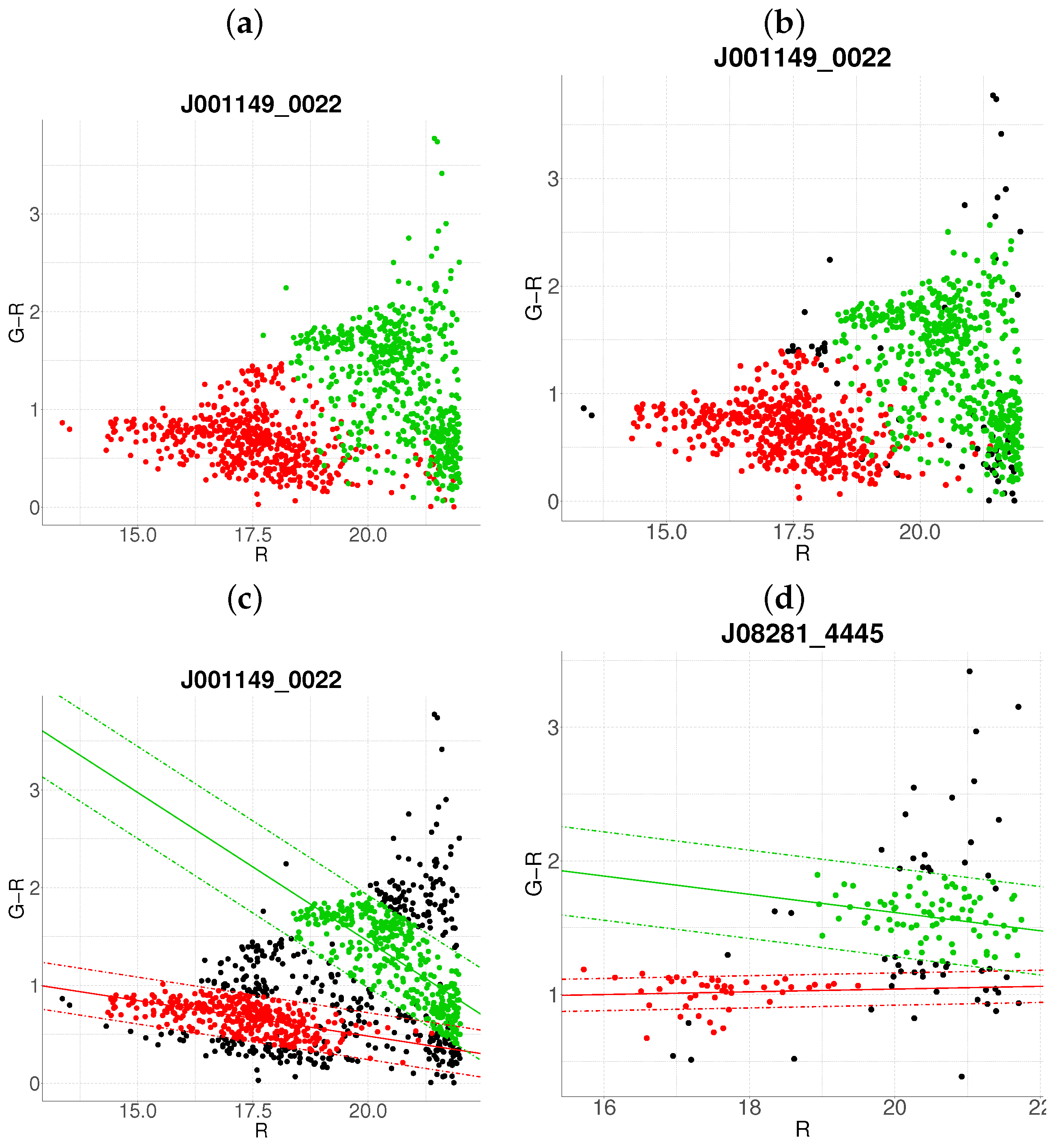
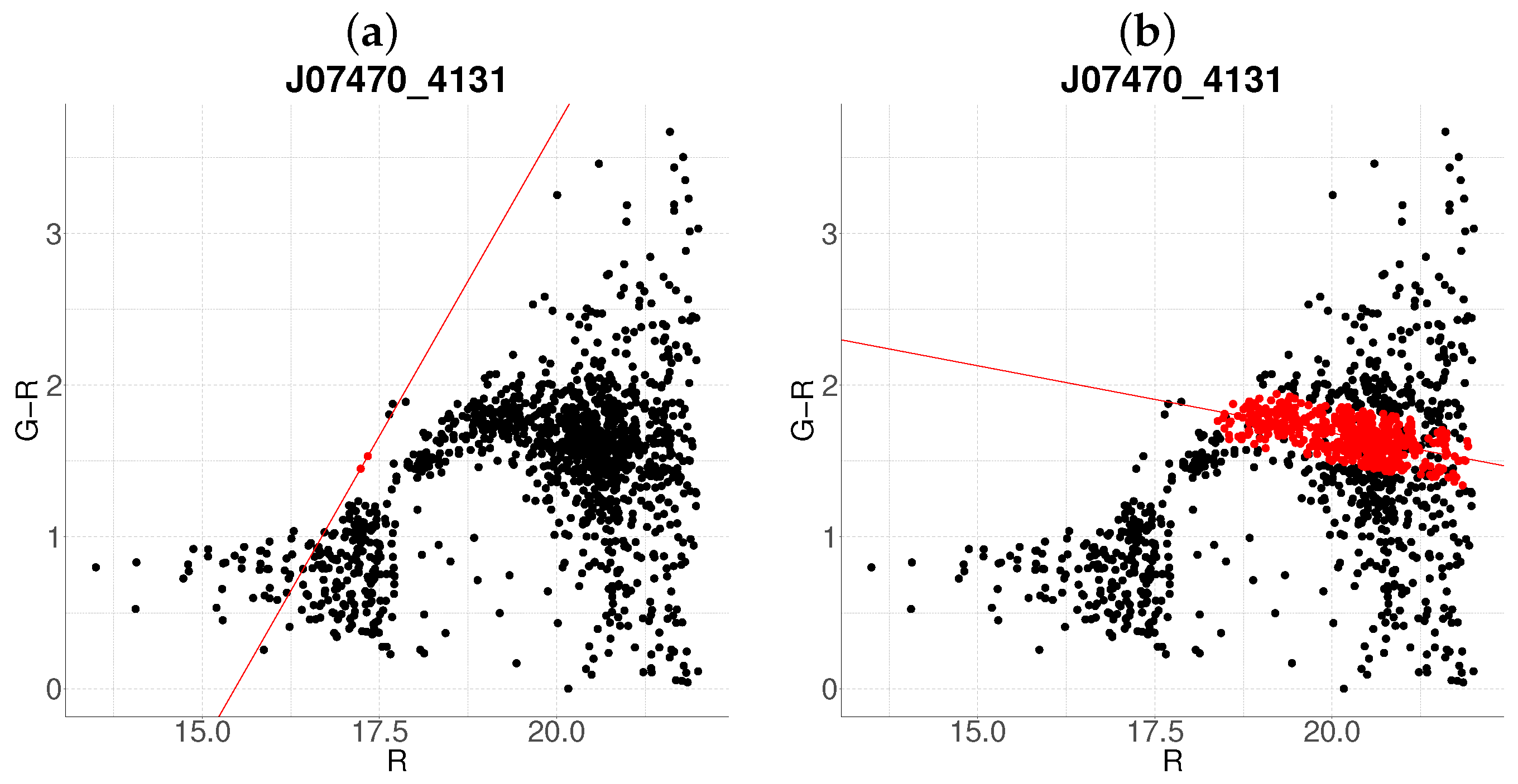
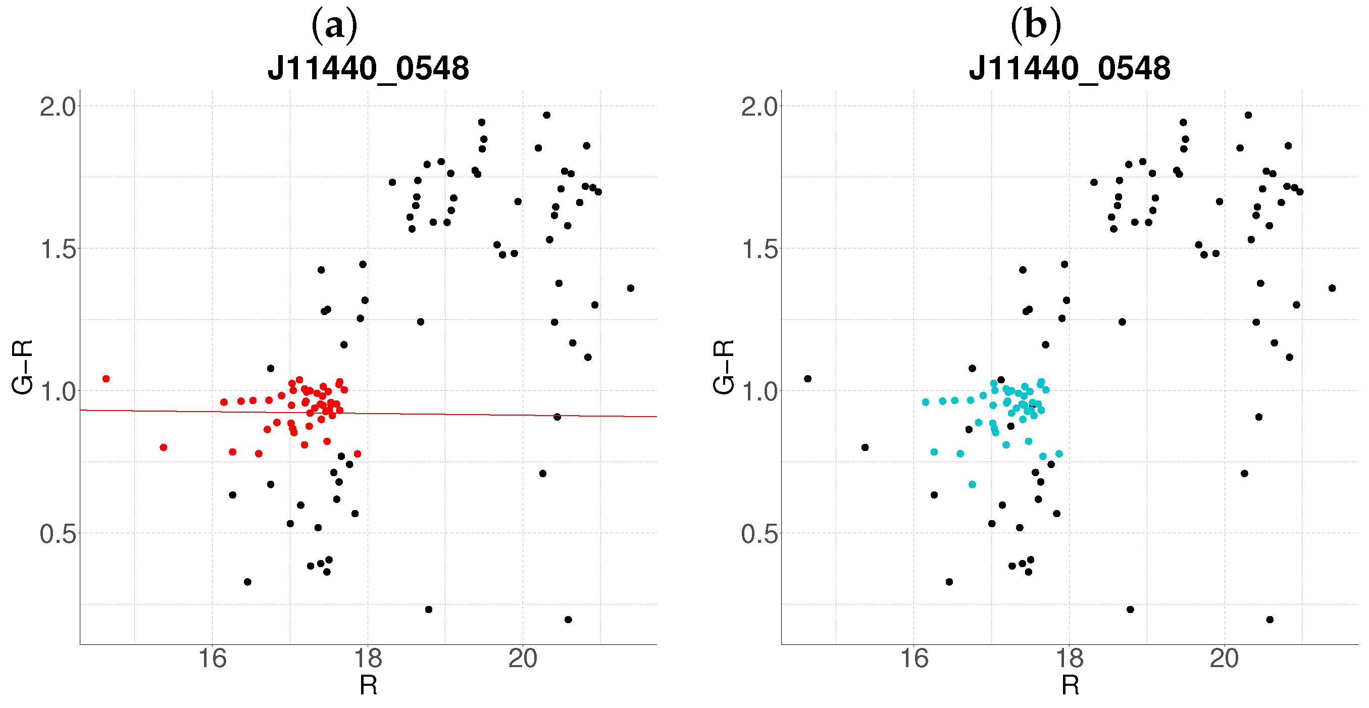
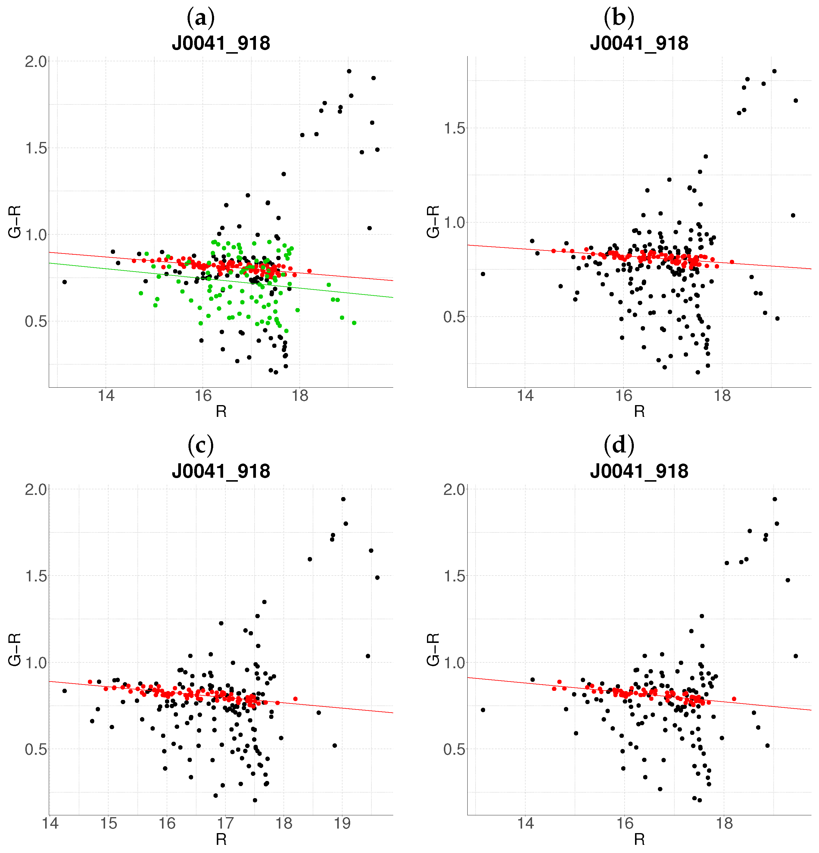
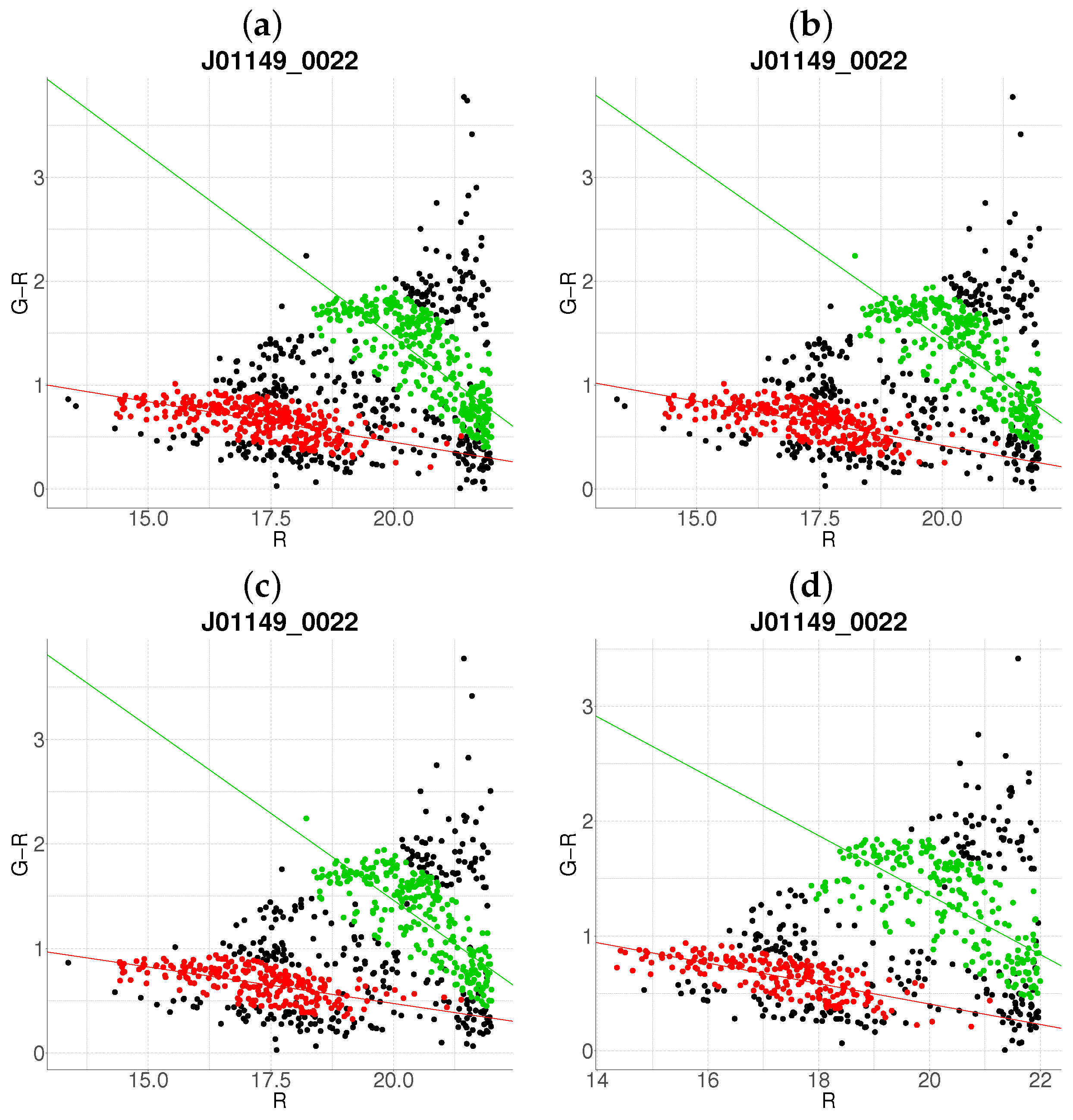
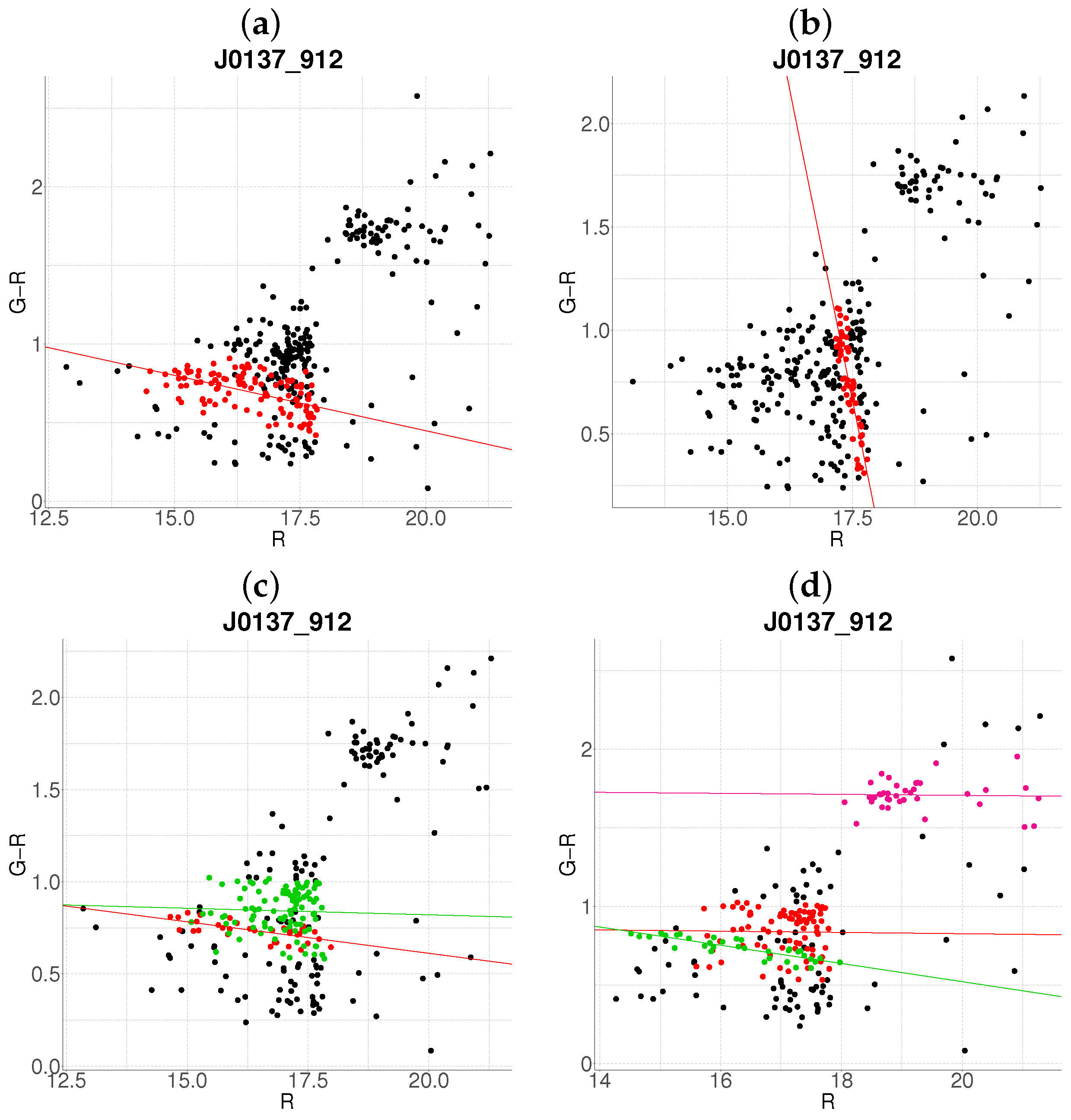
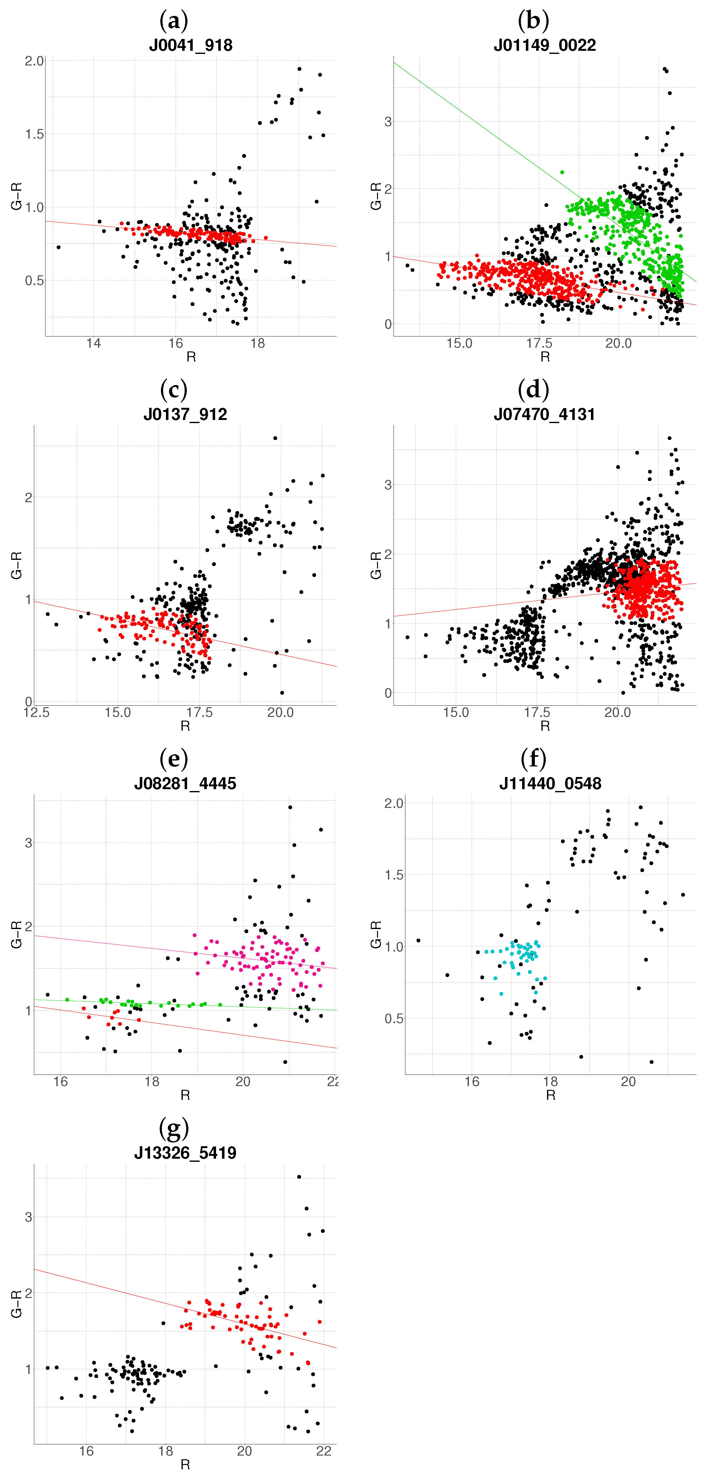
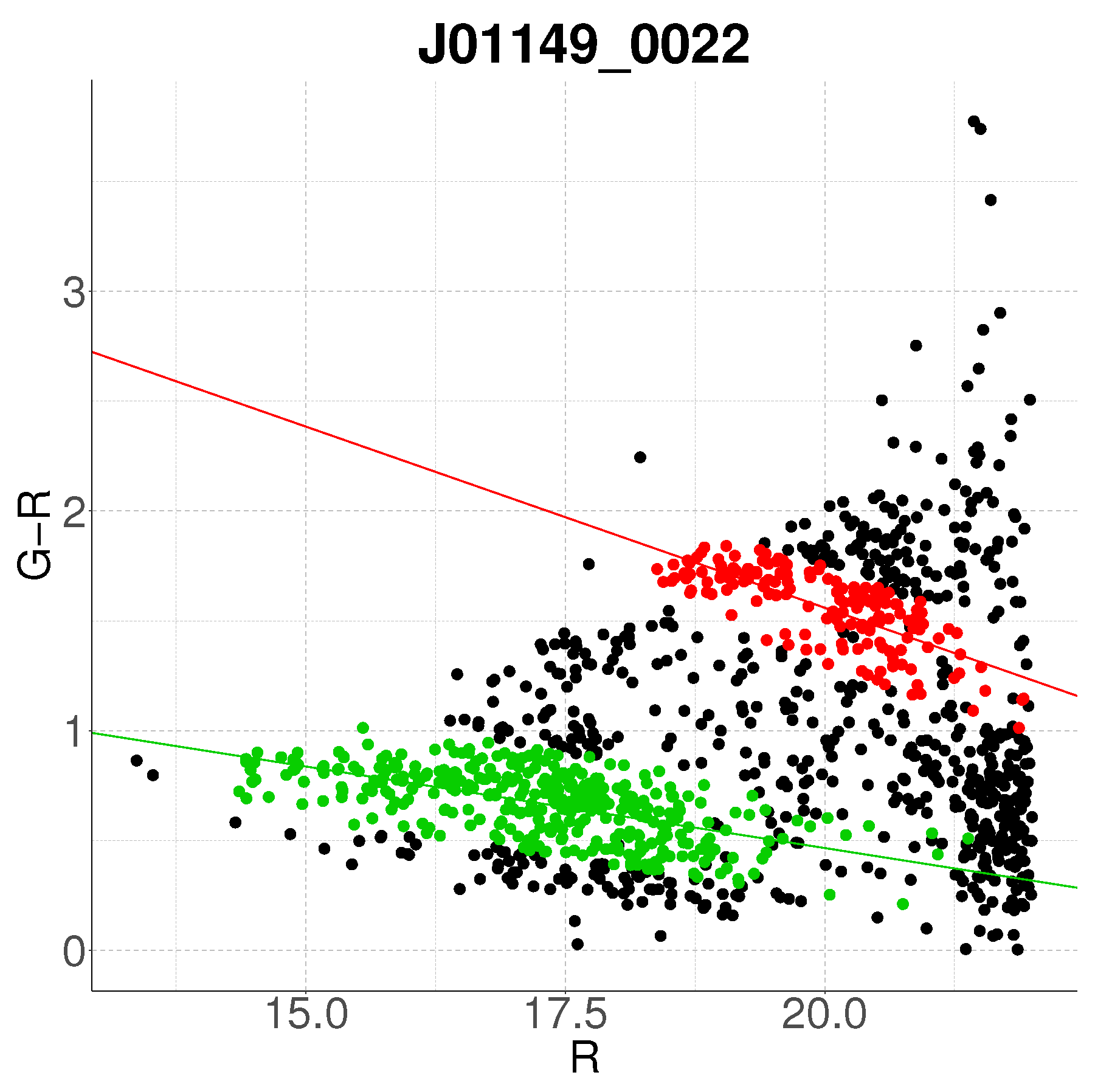
  • Step 1: Gaussian mixture modeling via EM algorithm
    The EM algorithm is applied to partition the dataset into two candidate subpopulations (cluster vs. background/foreground), modeling their multivariate distributions using Gaussian mixture models (GMMs). Parameters—including component means ( μ ), covariance matrices Σ , and mixture weights π —are optimized to maximize the likelihood of the observed data. Figure 1a illustrates this step for the cluster J001149-0022, where the initial classification assigns galaxies to two candidate components (red and green).
  • Step 2: Outlier rejection via Mahalanobis distance
    To mitigate contamination from interlopers, cluster membership is refined using a statistical threshold based on the Mahalanobis distance. A conservative cutoff is defined as the 95th percentile (0.95 quantile) of the χ 2 distribution with degrees of freedom equal to the dimensionality of the data (here, 3: r , g r , z ). Observations exceeding this threshold (black points in Figure 1b) are flagged as outliers and excluded from subsequent analysis.
  • Step 3: Projection and slope-based acceptance
    For each candidate cluster, the covariance matrix Σ is decomposed into its principal eigenvectors. The first eigenvector defines the dominant orientation (“slope”) of the cluster, while the second eigenvector quantifies intrinsic scatter perpendicular to this axis. Both eigenvectors define a plane in the 3D working enviroment, which we prioritize to capture maximal data variance. Two scenarios arise:
    • Negative slope (Red sequence compliance): A negative slope (characteristic of the red sequence) triggers the construction of an acceptance region. This region is bounded by lines offset from the principal axis by ± λ 2 , where λ 2 is the second eigenvalue of Σ (Figure 1c). Galaxies within these bounds are retained as high-confidence cluster members.
    • Non-negative slope (Iterative reassessment): A non-negative slope suggests spurious structure (e.g., projection effects). In such cases, the candidate with the smaller mean r-magnitude undergoes a second iteration (Steps 1–4). Persistent non-negative slopes after iteration lead to candidate rejection (e.g., red group in Figure 1d).
  • Step 4: Step control and qualitative comparison of results
    The algorithm terminates if at the first step, an acceptance region has been built, in another case, at the end of the second step. Final candidates are qualitatively compared against the results obtained with the base algorithm.

3. Results

A comparative evaluation of the base and proposed algorithms is illustrated in Figure 2, Figure 3, Figure 4, Figure 5, Figure 6, Figure 7 and Figure 8, which contrast their performance across seven galaxy clusters spanning a range of dynamical states and redshifts. Each figure pairs the output of the base algorithm (left panels) with the results of the proposed method (right panels).

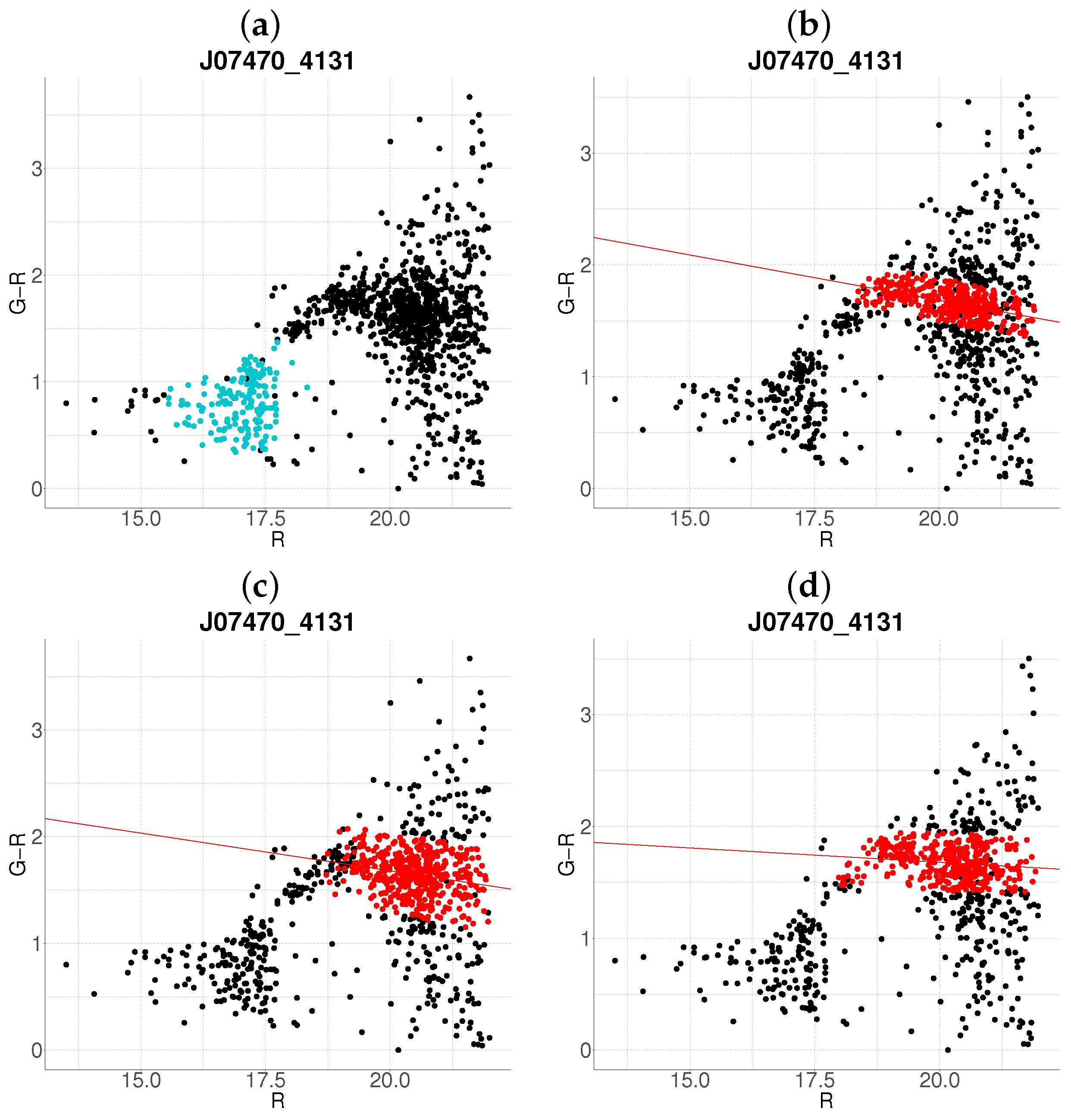
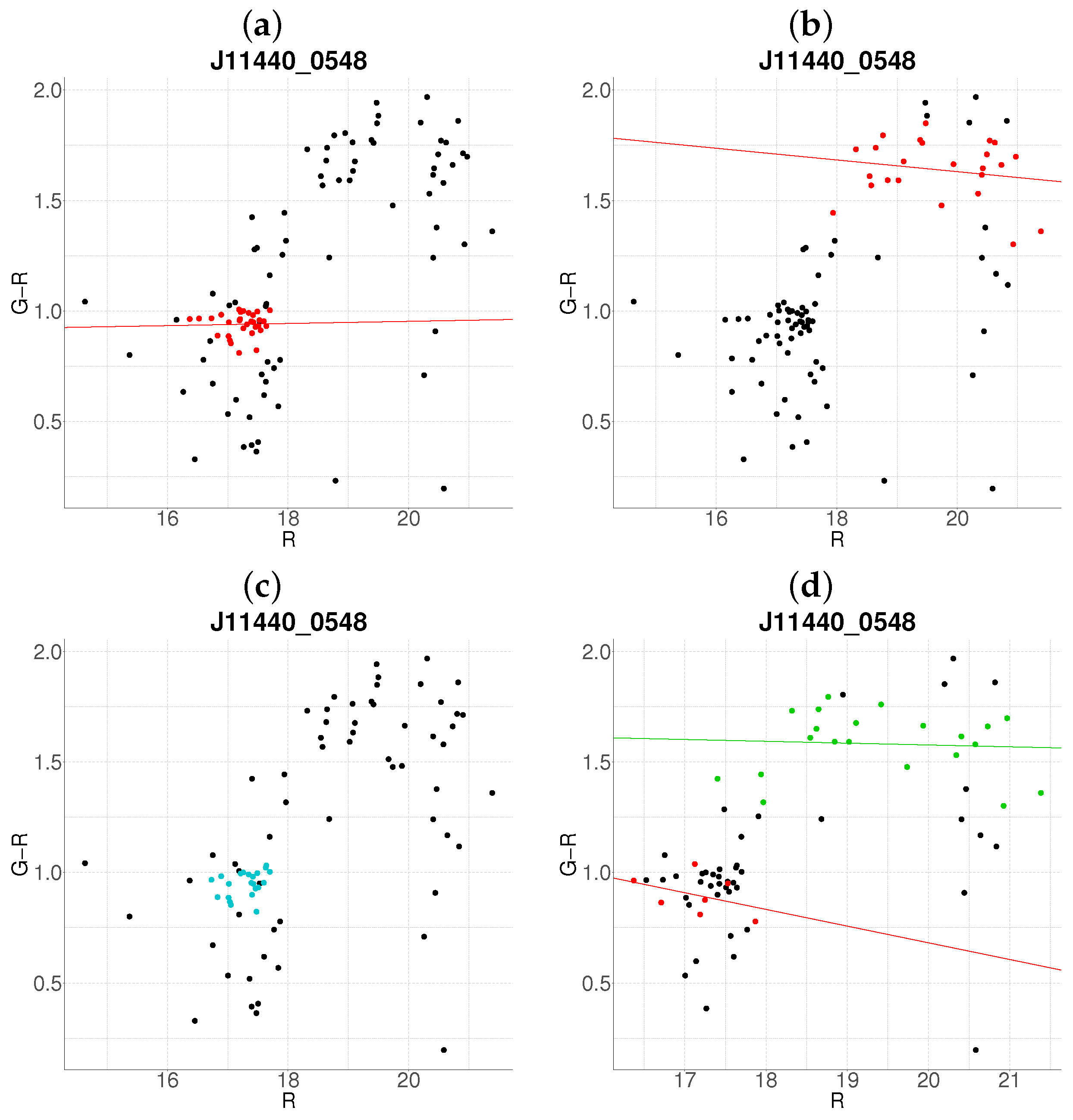
3.1. Cluster Detection and Membership Refinement

The proposed method prioritizes statistical reliability over membership counts, reducing contamination through multivariate thresholds (Figure 2b). In contrast, Figure 3b shows improved recovery of faint members in multi-cluster systems. A more striking contrast is evident in J0137-912 and J07470-4131, where the proposed algorithm successfully characterizes the clusters (Figure 4b and Figure 5b), whereas the base method fails to detect it entirely (Figure 4a and Figure 5a). This improvement is attributed to the integration of redshift constraints, which effectively filter foreground contamination.

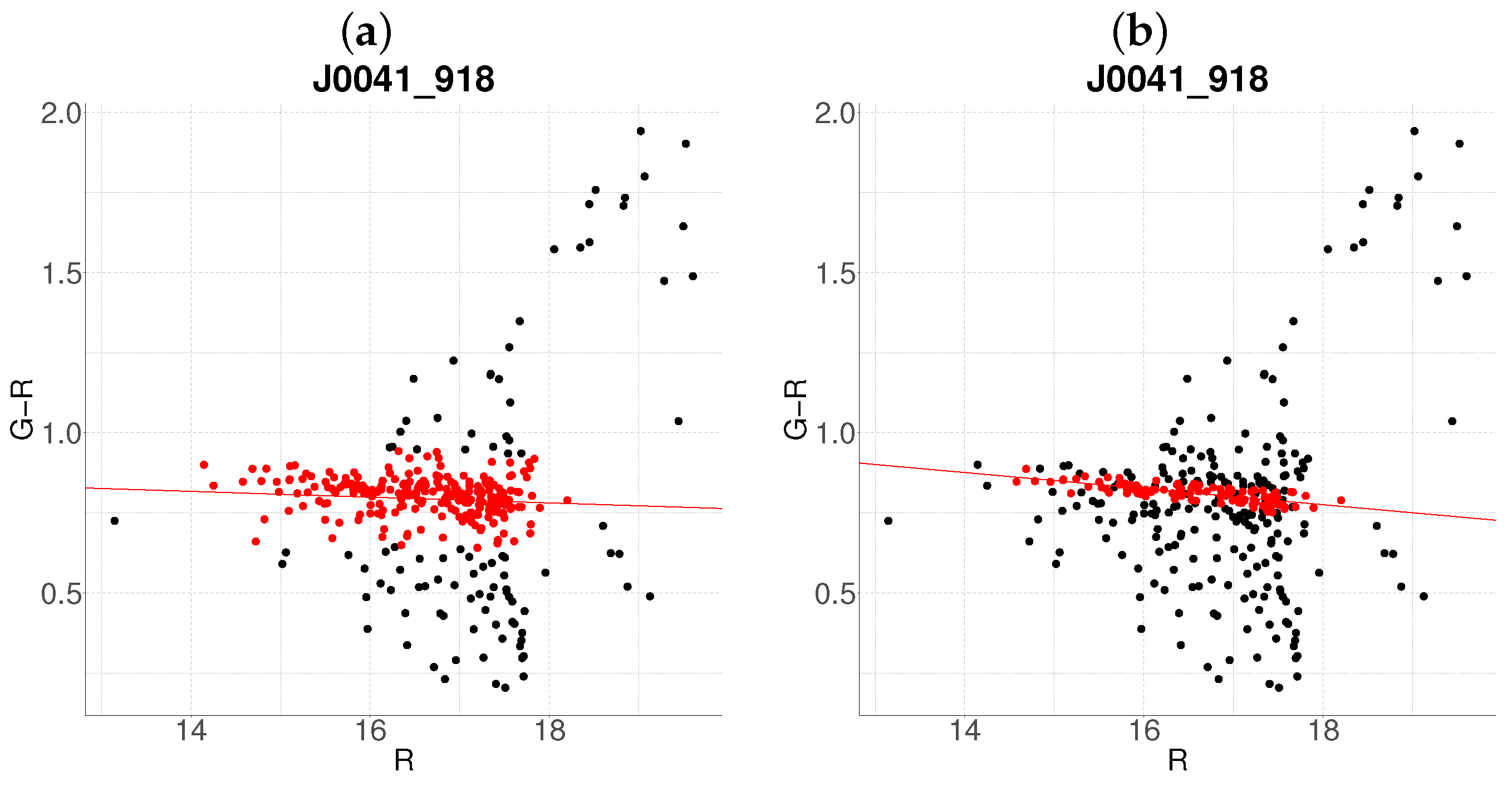
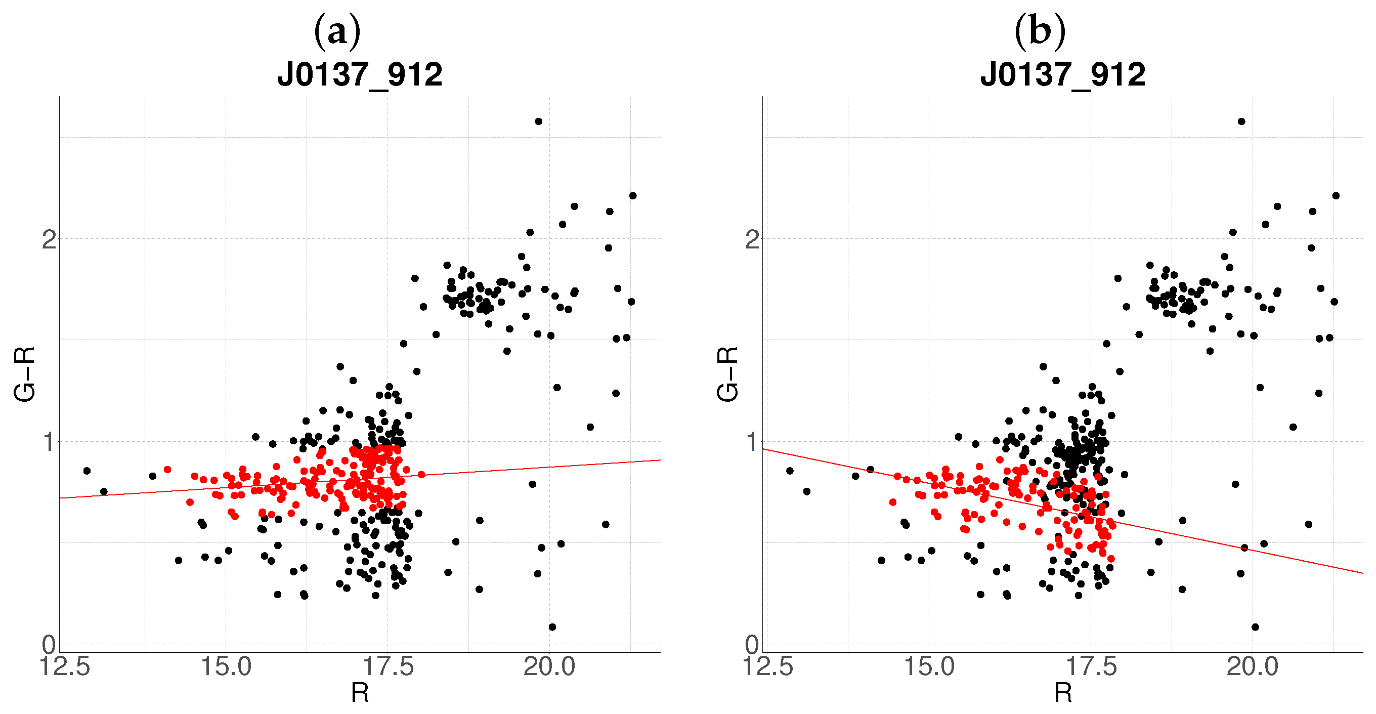
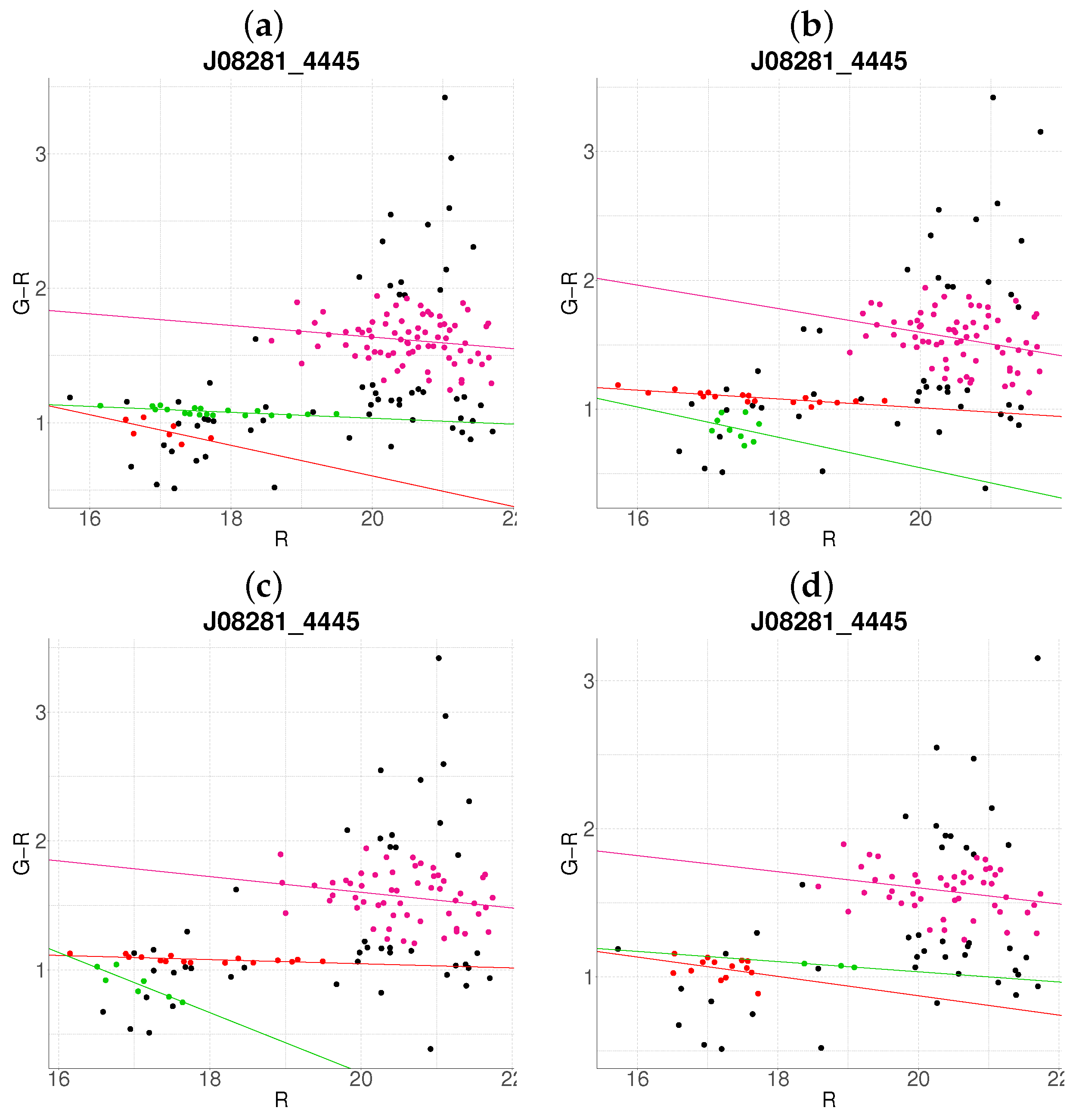
3.2. Resolution of Substructure and Multi-Cluster Detection

The method demonstrates enhanced sensitivity to substructure, as seen in J01149-0022 (Figure 3b), where it resolves two distinct clusters compared to the single overdensity detected by the base algorithm (Figure 3a). The primary cluster aligns with the base result but includes a broader membership, while the secondary cluster corresponds to a spectroscopically validated substructure. This improvement arises because the base algorithm, designed for single-cluster detection, cannot resolve substructures, unlike the proposed multivariate framework. Similarly, in J08281-4445, the proposed algorithm identifies three candidate clusters (Figure 6b), one of which matches the base detection (Figure 6a). It can also be seen that the cluster in purple present a mean redshift of z = 0.49 —this is an example of the behavior of the algorithm at high redshift regimes.

Edge Cases and Algorithm Limitations

While the proposed method excels in many scenarios, edge cases reveal areas for refinement. For instance, in J11440-0548, the algorithm identifies a group (blue points, Figure 7b) but refrains from classifying it as a cluster due to a non-negative slope—a conservative measure to reject projection effects. Conversely, in J13326-5419, the base algorithm achieves a correct characterization (Figure 8a), whereas the proposed method assigns an anomalous slope to the cluster (Figure 8b). This discrepancy arises from covariance between r-magnitude and redshift in the Gaussian mixture model, suggesting a need for special considerations in some cluster, (e.g., adjusting Mahalanobis thresholds.).

3.3. Robustness Test Against Data Loss and Photometric Redshift Noise

To evaluate the robustness of the proposed algorithm under incomplete data conditions, we systematically removed 10 % , 20 % , 30 % and 40 % of the elements from each sample through random sub-sampling, this test has been applied to seven sets here presented (J0041-918, J01149-0022, J0137-912, J07470-4131, J08281-4445, J11440-0548 y J13326-5419), the results are shown in Figure 9, Figure 10, Figure 11, Figure 12, Figure 13, Figure 14 and Figure 15. Figure 9 and Figure 10 demonstrate the algorithm’s stability (similar results in every cases): even at 40 % data loss, the detected cluster structures remain largely consistent with the original results (Figure 9b and Figure 10b), with the exception of a substructure (green) emerging in Figure 9.
For Figure 11, panel (a) ( 10 % reduction) shows no significant deviations from the reference (Figure 4b). However, panel (b) ( 20 % ) yields a nonsensical output (an exaggerated negative slope), likely due to the exclusion of critical cluster members in the 0.5 , 1   g r interval. At 30 % reduction (panel (c)), two distinct clusters are detected within the original cluster region, while panel (d) ( 40 % reduction) preserves this region but identifies an additional cluster in the 1.5 , 2   g r range.
In Figure 12, the algorithm fails to recover the reference cluster (Figure 5b) in panel a ( 10 % reduction), though it successfully detects clusters in panels b–d with minimal deviations. Figure 13 exhibits consistent results across all reduction levels, aside from expected population decreases and color variations.
Notably, Figure 14 reveals heightened sensitivity to data loss: panels b–d produce erratic outputs, suggesting instability in cluster definition for this sample. Conversely, Figure 15 shows remarkable resilience: the primary cluster (largest g r index) remains unaffected, and the algorithm even improves its detection of the secondary cluster near g r = 1 under partial data removal.
To evaluate the algorithm’s resilience to photometric redshift uncertainties, we introduced synthetic noise by perturbing redshift values uniformly across a range of −3000 to 3000 km s−1. After applying these perturbations, the algorithm was re-executed on the modified datasets. As shown in Figure 16, the method demonstrates consistent performance in most cases: panels a, b, c, e, and f exhibit nearly identical cluster recovery compared to noise-free results.
Notable deviations occur in panel d, where the detected cluster’s slope diverges from expectations (cf. Figure 5b), though its spatial boundaries align with the original detection. Panel g reveals partial sensitivity: while the cluster near g r = 1 is lost, the structure within 1 , 2 remains almost the same.

4. Discussion

Beforehand, we must mention that an implementation in R of the algorithm is provided in Appendix A at the end of this work. All the results obtained in this work were obtained using a computer program, and it is provided herein for the sake of transparency.
While the proposed method demonstrates improved discrimination of cluster members in certain cases (e.g., J0137-912, Figure 4b), it does not universally assign a larger population of galaxies to clusters compared to the base algorithm. For instance, in J0041-918 (Figure 2), the proposed method retains fewer galaxies but with tighter redshift consistency, prioritizing statistical reliability over sheer membership counts. This reflects the algorithm’s core principle: probabilistic classification via Mahalanobis distance and GMMs, which inherently penalizes outliers and foreground/background interlopers. Thus, the method’s strength lies not in maximizing membership numbers, but in leveraging multivariate criteria (color, magnitude, redshift) to statistically validate members. This approach ensures robustness against projection effects, even if it occasionally reduces the apparent richness of clusters.
Conversely, Figure 3 highlights scenarios where the multivariate framework enhances sensitivity. In panel b, the proposed algorithm detects a statistically robust overdensity by incorporating galaxies dismissed as outliers in the base method (panel a). This improvement arises from the Mahalanobis distance’s ability to account for covariance between variables, enabling probabilistic membership assignments that transcend rigid Euclidean thresholds. Notably, the secondary cluster in panel b exhibits a steeper slope and larger scatter, likely due to its higher redshift ( z = 0.34 ), underscoring the need for redshift-specific parameter tuning to address biases in high-z regimes.
Furthermore, the algorithm’s capacity to resolve multiple clusters within a single field (e.g., Figure 3b, Figure 6b and Figure 8b) positions it as a powerful exploratory tool for identifying substructure or neighboring systems. This capability is particularly valuable for studies of cluster mergers and large-scale structure, where disentangling overlapping populations is critical [32]. To demonstrate this adaptability, we applied the algorithm once again to the initial clustering solution in Figure 3b. The refined output (Figure 17) reveals a more physically plausible slope for the green cluster, underscoring the method’s potential to enhance preliminary results through reprocessing. This suggests that even robust initial detections may benefit from targeted reanalysis.
The algorithm also corrects systematic biases inherent to slope estimation in the base method. For instance, in Figure 4b, the revised red sequence slope aligns more closely with theoretical expectations for passively evolving populations [6], whereas the base algorithm’s fit (panel a) deviates due to contamination. Similarly, the detection of J07470-4131 (Figure 5b) demonstrates improved handling of ambiguous color–magnitude distributions, which previously eluded classification. These enhancements stem from the principal eigenvector-derived slope, which adaptively reflects the intrinsic scatter and orientation of the cluster in parameter space.
The algorithm’s performance under two critical stress scenarios—data incompleteness and photometric redshift noise—reveals both its strengths and limitations as a tool for cluster detection in heterogeneous datasets. The algorithm maintains structural coherence even under significant data loss (up to 40 % random subsampling). This robustness is particularly evident in Figure 9 and Figure 15, where primary clusters remain identifiable despite population reductions. However, the emergence of spurious substructures (e.g., Figure 11c) and failures in recovering critical clusters (e.g., Figure 14b–d) highlight a dependency on representative sampling.
The introduction of synthetic redshift perturbations ( ± 3000  km s−1) tested the algorithm’s ability to disentangle clusters in noisy environments. While positional stability persisted in most cases (Figure 16a–c,e,f), distortions in slope (Figure 16d) and partial cluster loss (Figure 16g) underscore the method’s sensitivity to redshift-driven degeneracies. This suggests that while spatial coherence is robust to noise, kinematic features are more susceptible to photometric uncertainties.
The combined results indicate that the algorithm prioritizes spatial over kinematic fidelity under data degradation, making it suitable for large-area surveys where completeness is prioritized over precision (e.g., SDSS, DES). However, its limitations in noisy or incomplete regimes necessitate caution in studies requiring dynamical interpretations (e.g., merger kinematics). A practical compromise involves hybrid approaches: using this method for initial detections in photometric surveys, followed by spectroscopic refinement for critical subsamples.
Despite these advancements, the algorithm exhibits limitations in edge cases. In Figure 7b, the failure to classify a candidate cluster—despite its morphological resemblance to panel a—may reflect overconservative slope criteria or unresolved covariance between variables. Similarly, the mischaracterization of J13326-5419 (Figure 8b) suggests that some clusters may require tailored parameterization to account for redshift-dependent selection effects and luminosity function evolution. These challenges highlight two priorities for future work. The first one is a parameter optimization via dynamic adjustment of Mahalanobis distance thresholds and slope criteria based on cluster redshift and richness, and the second one should be a hybrid validation which could integrate spectroscopic follow-up or weak-lensing mass maps to refine probabilistic membership assignments [33].

5. Conclusions

This study presents a novel algorithm for galaxy cluster characterization that synergizes the well-established red sequence technique with advanced statistical classification methods. By incorporating Gaussian mixture models (GMMs) and Mahalanobis distance discrimination across three dimensions (r-magnitude, g r color and redshift z), the algorithm achieves robust and often superior performance compared to traditional bivariate approaches. The integration of redshift as a classification criterion proved particularly impactful, mitigating contamination from foreground/background galaxies and refining membership determination—a critical advancement for photometric surveys where spectroscopic follow-up is limited.
The algorithm’s ability to resolve multiple clusters within a single field (e.g., J01149-0022, J08281-4445) and recover previously undetected systems (e.g., J0137-912) underscores its utility as an exploratory tool for large-scale surveys. These capabilities position it as a promising candidate for deployment in next-generation projects like LSST and Euclid, where automated, scalable cluster detection is paramount.
Future work should prioritize optimizing the algorithm for high-richness systems, where deviations from Gaussian assumptions in covariance structures may necessitate computational refinements. Additionally, integrating supervised learning techniques—such as convolutional neural networks for spatial overdensity detection—could enhance outlier rejection and slope calibration, bridging the gap between unsupervised statistical methods and astrophysical intuition. By advancing these avenues, the algorithm offers a pathway to unraveling the complex interplay between galaxy evolution and dark matter halo assembly, reinforcing its role in precision cosmology.

Author Contributions

Conceptualization, J.A.G.-D.-d.-L. and J.E.M.-D.; methodology, D.R.M.-R., J.J.T.-A., J.A.G.-D.-d.-L. and J.E.M.-D.; software, D.R.M.-R., J.J.T.-A., J.A.G.-D.-d.-L. and J.E.M.-D.; validation, D.R.M.-R., J.J.T.-A., J.A.G.-D.-d.-L. and J.E.M.-D.; formal analysis, D.R.M.-R.; investigation, D.R.M.-R., J.J.T.-A., J.A.G.-D.-d.-L. and J.E.M.-D.; resources, D.R.M.-R., J.J.T.-A., J.A.G.-D.-d.-L. and J.E.M.-D.; data curation, J.J.T.-A., J.A.G.-D.-d.-L. and J.E.M.-D.; writing—original draft preparation, D.R.M.-R., J.J.T.-A., J.A.G.-D.-d.-L. and J.E.M.-D.; writing—review and editing, D.R.M.-R., J.J.T.-A., J.A.G.-D.-d.-L. and J.E.M.-D.; visualization, D.R.M.-R.; supervision, J.J.T.-A., J.A.G.-D.-d.-L. and J.E.M.-D. All authors have read and agreed to the published version of the manuscript.

Funding

This research received no external funding.

Institutional Review Board Statement

Not applicable.

Informed Consent Statement

Not applicable.

Data Availability Statement

The raw data supporting the conclusions of this article will be made available by the authors on request.

Conflicts of Interest

The authors declare no conflicts of interest.

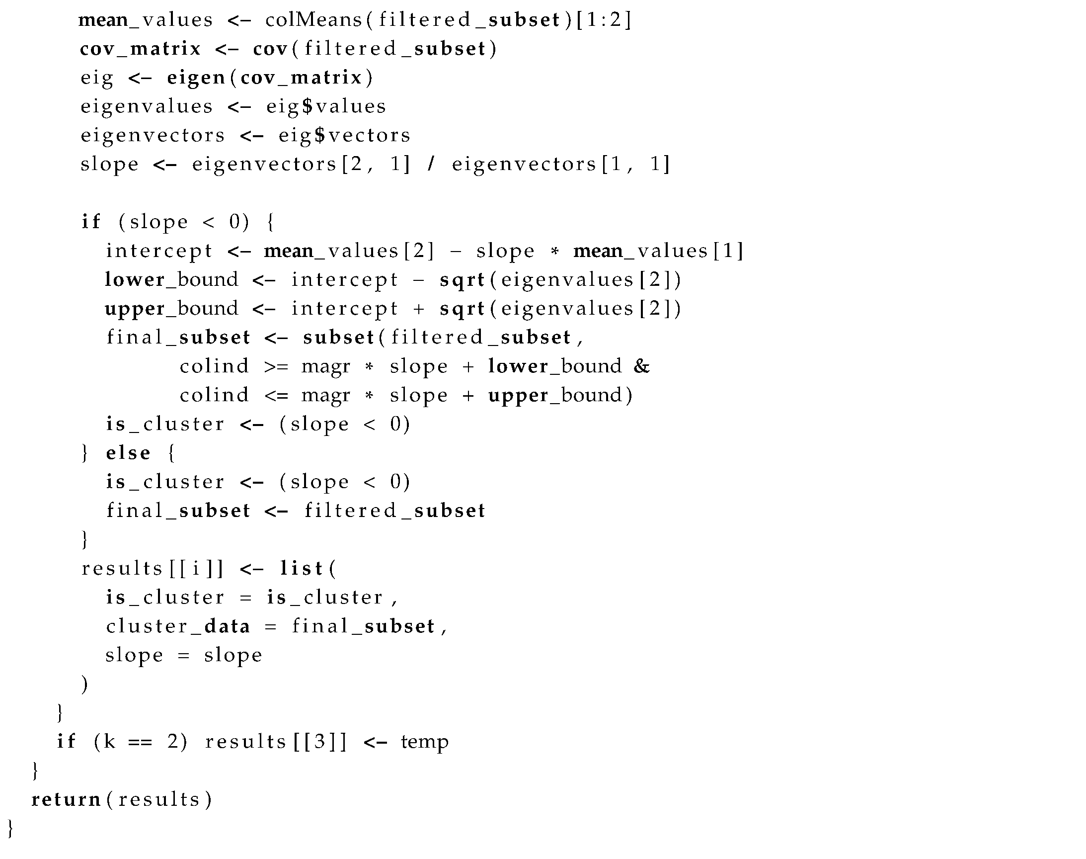
Appendix A. Computer Code

In this appendix, we provide the computer code used to carry out the data analyses presented in this work. It is worth pointing out that the code was written in R. We provide it here for the readers to reproduce our simulations and to carry out simulations themselves.
Galaxies 13 00052 i001
Galaxies 13 00052 i002
Galaxies 13 00052 i003

References

  1. Rines, K.; Geller, M.J.; Diaferio, A.; Kurtz, M.J. Measuring the ultimate halo mass of galaxy clusters: Redshifts and mass profiles from the hectospec cluster survey (hecs). Astrophys. J. 2013, 767, 15. [Google Scholar] [CrossRef]
  2. Baum, W.A. Population Inferences from Star Counts, Surface Brightness and Colors. Publ. Astron. Soc. Pac. 1959, 71, 106–117. [Google Scholar] [CrossRef]
  3. Faber, S.M.; Jackson, R.E. Velocity dispersions and mass-to-light ratios for elliptical galaxies. Astrophys. J. 1976, 204, 668–683. [Google Scholar] [CrossRef]
  4. Dressler, A.; Lynden-Bell, D.; Burstein, D.; Davies, R.L.; Faber, S.M.; Terlevich, R.; Wegner, G. Spectroscopy and Photometry of Elliptical Galaxies. I. New Distance Estimator. Astrophys. J. 1987, 313, 42–58. [Google Scholar] [CrossRef]
  5. Blanton, M.R.; Hogg, D.W.; Bahcall, N.A.; Baldry, I.K.; Brinkmann, J.; Csabai, I.; Eisenstein, D.; Fukugita, M.; Gunn, J.E.; Ivezić, V.; et al. The Broadband Optical Properties of Galaxies with Redshifts 0.02<z<0.22. Astrophys. J. 2003, 594, 186–207. [Google Scholar]
  6. López-Cruz, O.; Barkhouse, W.A.; Yee, H. The color-magnitude effect in early-type cluster galaxies. Astrophys. J. 2004, 614, 679. [Google Scholar] [CrossRef]
  7. Hogg, D.W.; Blanton, M.R.; Brinchmann, J.; Eisenstein, D.J.; Schlegel, D.J.; Gunn, J.E.; McKay, T.A.; Rix, H.W.; Bahcall, N.A.; Brinkmann, J.; et al. The Dependence on Environment of the Color-Magnitude Relation of Galaxies. Astrophys. J. Lett. 2004, 601, L29–L32. [Google Scholar] [CrossRef]
  8. Cerulo, P.; Orellana, G.A.; Covone, G. The evolution of brightest cluster galaxies in the nearby Universe – I. Colours and stellar masses from the Sloan Digital Sky Survey and Wide Infrared Survey Explorer. Mon. Not. R. Astron. Soc. 2019, 487, 3759–3775. [Google Scholar] [CrossRef]
  9. Khanday, S.A.; Saha, K.; Iqbal, N.; Dhiwar, S.; Pahwa, I. Morphology, colour–magnitude, and scaling relations of galaxies in Abell 426. Mon. Not. R. Astron. Soc. 2022, 515, 5043–5061. [Google Scholar] [CrossRef]
  10. Hahn, C.; Bottrell, C.; Lee, K.G. HaloFlow. I. Neural Inference of Halo Mass from Galaxy Photometry and Morphology. Astrophys. J. 2024, 968, 968–990. [Google Scholar] [CrossRef]
  11. Yantovski-Barth, M.J.; Newman, J.A.; Dey, B.; Andrews, B.H.; Eracleous, M.; Golden-Marx, J.; Zhou, R. The CluMPR galaxy cluster-finding algorithm and DESI legacy survey galaxy cluster catalogue. Mon. Not. R. Astron. Soc. 2024, 531, 2285–2303. [Google Scholar] [CrossRef]
  12. Gladders, M.D.; Yee, H. A new method for galaxy cluster detection. I. The algorithm. Astron. J. 2000, 120, 2148. [Google Scholar] [CrossRef]
  13. Trejo-Alonso, J.; Caretta, C.; Laganá, T.F.; Sodré Jr, L.; Cypriano, E.S.; Lima Neto, G.; Mendes de Oliveira, C. Red sequence of Abell X-ray underluminous clusters. Mon. Not. R. Astron. Soc. 2014, 441, 776–783. [Google Scholar] [CrossRef]
  14. Mares, D.; Trejo, J.; Díaz, A. Determinación de Membresía por las Técnicas de Secuencia Roja y Cáusticas; Technical report, 25 Verano de la Ciencia Región Centro; Academia Mexicana de Ciencia: Queretaro, Mexico, 2023. [Google Scholar]
  15. McLachlan, G.J.; Lee, S.X.; Rathnayake, S.I. Finite Mixture Models. Annu. Rev. Stat. Appl. 2019, 6, 355–378. [Google Scholar] [CrossRef]
  16. Sarria, M.; Castellanos, G. Entrenamiento discriminativo por distancia de Mahalanobis para detección de patologías de voz. Dyna 2010, 77, 220–228. [Google Scholar]
  17. Pearson, K. Contributions to the Mathematical Theory of Evolution. Philos. Trans. R. Soc. Lond. A 1894, 185, 71–110. [Google Scholar]
  18. Rao, C.R. The Utilization of Multiple Measurements in Problems of Biological Classification. J. R. Stat. Soc. Ser. (Methodol.) 1948, 10, 159–203. [Google Scholar] [CrossRef]
  19. Hasselblad, V. Estimation of Parameters for a Mixture of Normal Distributions. Technometrics 1966, 8, 431–444. [Google Scholar] [CrossRef]
  20. Gensler, S. Finite Mixture Models. In Handbook of Market Research; Homburg, C., Klarmann, M., Vomberg, A., Eds.; Springer International Publishing: Cham, Switzerland, 2022; pp. 251–264. [Google Scholar] [CrossRef]
  21. Burgett, W.S.; Vick, M.M.; Davis, D.S.; Colless, M.; De Propris, R.; Baldry, I.; Baugh, C.; Bland-Hawthorn, J.; Bridges, T.; Cannon, R.; et al. Substructure analysis of selected low-richness 2dFGRS clusters of galaxies. Mon. Not. R. Astron. Soc. 2004, 352, 605–654. [Google Scholar] [CrossRef]
  22. Dempster, A.P.; Laird, N.M.; Rubin, D.B. Maximum Likelihood from Incomplete Data Via the EM Algorithm. J. R. Stat. Soc. Ser. B (Methodol.) 1977, 39, 1–22. [Google Scholar] [CrossRef]
  23. Portillo, M.T.E.; Plata, J.A.S. P. Ch. Mahalanobis y las aplicaciones de su distancia estadística. CULCyT: Cult. Cient. Tecnol. 2008, 5, 13–20. [Google Scholar]
  24. Gómez Silva, M.J.; Armingol, J.M.; Escalera, A.d.l. Re-identificación de personas mediante la distancia de Mahalanobis. In Proceedings of the XXXIX Jornadas de Automática, Área de Ingeniería de Sistemas y Automática, Universidad de Extremadura, Badajoz, Spain, 5–7 September 2018; pp. 967–974. [Google Scholar]
  25. Popesso, P.; Böhringer, H.; Brinkmann, J.; Voges, W.; York, D.G. RASS-SDSS Galaxy clusters survey-I. The catalog and the correlation of X-ray and optical properties. Astron. Astrophys. 2004, 423, 449–467. [Google Scholar] [CrossRef]
  26. Aihara, H.; Prieto, C.; An, D.; Anderson, S.; Aubourg, E.; Balbinot, E.; Beers, T.; Berlind, A.A.; Bickerton, S.; Bizyaev, D.; et al. The eighth data release of the Sloan Digital Sky Survey: First data from SDSS-III. Astrophys. J. Suppl. Ser. 2011, 193, 29. [Google Scholar] [CrossRef]
  27. Alam, S.; Albareti, F.; Prieto, C.; Anders, F.; Anderson, S.; Anderton, T.; Andrews, B.; Armengaud, E.; Aubourg, É.; Bailey, S.; et al. The eleventh and twelfth data releases of the Sloan Digital Sky Survey: Final data from SDSS-III. Astrophys. J. Suppl. Ser. 2015, 219, 12. [Google Scholar] [CrossRef]
  28. Strauss, M.; Weinberg, D.; Lupton, R.; Narayanan, V.; Annis, J.; Bernardi, M.; Blanton, M.; Burles, S.; Connolly, A.; Dalcanton, J.; et al. Spectroscopic target selection in the Sloan Digital Sky Survey: The main galaxy sample. Astron. J. 2002, 124, 1810. [Google Scholar] [CrossRef]
  29. Stoughton, C.; Lupton, R.; Bernardi, M.; Blanton, M.; Burles, S.; Castander, F.; Connolly, A.; Eisenstein, D.; Frieman, J.; Hennessy, G.; et al. Sloan digital sky survey: Early data release. Astron. J. 2002, 123, 485. [Google Scholar] [CrossRef]
  30. Koester, B.P.; McKay, T.A.; Annis, J.; Wechsler, R.H.; Evrard, A.; Bleem, L.; Becker, M.; Johnston, D.; Sheldon, E.; Nichol, R.; et al. A MaxBCG catalog of 13,823 galaxy clusters from the sloan digital sky survey. Astrophys. J. 2007, 660, 239. [Google Scholar] [CrossRef]
  31. Venables, W.; Ripley, B.; Venables, W.; Ripley, B. Linear statistical models. In Modern Applied Statistics with S; Series Statistics and Computing; Springer: New York, NY, USA, 2002; pp. 139–181. [Google Scholar]
  32. Li, H.; Vogelsberger, M.; Bryan, G.L.; Marinacci, F.; Sales, L.V.; Torrey, P. Formation and evolution of young massive clusters in galaxy mergers: The SMUGGLE view. Mon. Not. R. Astron. Soc. 2022, 514, 265–279. [Google Scholar] [CrossRef]
  33. Murray, C.; Bartlett, J.G.; Artis, E.; Melin, J.B. Measuring weak lensing masses on individual clusters. Mon. Not. R. Astron. Soc. 2022, 512, 4785–4791. [Google Scholar] [CrossRef]
Figure 1. Proposed algorithm steps applied to J001149-0022 (a) Step 1, (b) Step 2 and (c) Step 3 case 1. In (d) Step 3 case 2 is applied to J08281-4445. In all panels, background and foreground galaxies are denoted in black, high-confidence cluster members in red, green, or pink (with a fitted red sequence line), and unclassified groups or substructures in blue.
Galaxies 13 00052 g001
Figure 2. Comparative between algorithms (a) J0041-918 with the base algorithm. (b) J0041-918 with the proposed algorithm ( z = 0.06 ). The color code is the same as in Figure 1.
Galaxies 13 00052 g002
Figure 3. Comparative between algorithms (a) J01149-0022 with the base algorithm. (b) J01149-0022 with the proposed algorithm ( z R = 0.08 , z G = 0.56 ). The color code is the same as in Figure 1.
Galaxies 13 00052 g003
Figure 4. Comparative between algorithms (a) J0137-912 with the base algorithm. (b) J0137-912 with the proposed algorithm ( z = 0.07 ). The color code is the same as in Figure 1.
Galaxies 13 00052 g004
Figure 5. Comparative between algorithms (a) J07470-4131 with the base algorithm. (b) J07470-4131 with the proposed algorithm ( z = 0.49 ). The color code is the same as in Figure 1.
Galaxies 13 00052 g005
Figure 6. Comparative between algorithms (a) J08281-4445 with the base algorithm. (b) J08281-4445 with the proposed algorithm ( z R = 0.15 , z G = 0.5 ). The color code is the same as in Figure 1.
Galaxies 13 00052 g006
Figure 7. Comparative between algorithms (a) J11440-0548 with the base algorithm. (b) J11440-0548 with the proposed algorithm ( z = 0.1 ). The color code is the same as in Figure 1.
Galaxies 13 00052 g007
Figure 8. Comparative between algorithms (a) J13326-5419 with the base algorithm. (b) J13326-5419 with the proposed algorithm ( z R = 0.11 , z G = 0.48 ). The color code is the same as in Figure 1.
Galaxies 13 00052 g008
Figure 9. Robustness test of the proposed algorithm on a randomly subsampled population of J0041-918. Panels (ad) show results with 10–40% data removal, respectively. The color code is the same as in Figure 1.
Galaxies 13 00052 g009
Figure 10. Robustness test of the proposed algorithm on a randomly subsampled population of J01149-0022. Panels (ad) show results with 10–40% data removal, respectively. The color code is the same as in Figure 1.
Galaxies 13 00052 g010
Figure 11. Robustness test of the proposed algorithm on a randomly subsampled population of J0137-912. Panels (ad) show results with 10–40% data removal, respectively. The color code is the same as in Figure 1.
Galaxies 13 00052 g011
Figure 12. Robustness test of the proposed algorithm on a randomly subsampled population of J07470-4131. Panels (ad) show results with 10–40% data removal, respectively. The color code is the same as in Figure 1.
Galaxies 13 00052 g012
Figure 13. Robustness test of the proposed algorithm on a randomly subsampled population of J08281-4445. Panels (ad) show results with 10–40% data removal, respectively. The color code is the same as in Figure 1.
Galaxies 13 00052 g013
Figure 14. Robustness test of the proposed algorithm on a randomly subsampled population of J11440-0548. Panels (ad) show results with 10–40% data removal, respectively. The color code is the same as in Figure 1.
Galaxies 13 00052 g014
Figure 15. Robustness test of the proposed algorithm on a randomly subsampled population of J13326-5419. Panels (ad) show results with 10–40% data removal, respectively. The color code is the same as in Figure 1.
Galaxies 13 00052 g015
Figure 16. Proposed algorithm applied to (a) J0041-918, (b) J01149-0022, (c) J0137-912, (d) J07470-4131, (e) J08281-4445, (f) J11440-0548, (g) J13326-5419 with artificial random noise introduced to the velocity data ± 3000 km s−1. The color code is the same as in Figure 1.
Galaxies 13 00052 g016
Figure 17. The algorithm is been applied once again over J01149-0022 giving a refined result. The color code is the same as in Figure 1.
Galaxies 13 00052 g017
Disclaimer/Publisher’s Note: The statements, opinions and data contained in all publications are solely those of the individual author(s) and contributor(s) and not of MDPI and/or the editor(s). MDPI and/or the editor(s) disclaim responsibility for any injury to people or property resulting from any ideas, methods, instructions or products referred to in the content.

