Article

PyMAP: Python-Based Data Analysis Package with a New Image Cleaning Method to Enhance the Sensitivity of MACE Telescope

by
Mani Khurana
1,2,*,
Kuldeep Kumar Yadav
1,2,
Pradeep Chandra
1,*,
Krishna Kumar Singh
1,2,
Atul Pathania
1,2 and
Chinmay Borwankar
1,*
1
Astrophysical Sciences Division, Bhabha Atomic Research Centre, Mumbai 400085, India
2
Homi Bhabha National Institute, Anushakti Nagar, Mumbai 400094, India
*
Authors to whom correspondence should be addressed.
Galaxies 2025, 13(1), 14; https://doi.org/10.3390/galaxies13010014
Submission received: 6 November 2024 / Revised: 10 February 2025 / Accepted: 11 February 2025 / Published: 15 February 2025

Abstract

:
Observations of Very High Energy (VHE) gamma ray sources using the ground-based Imaging Atmospheric Cherenkov Telescopes (IACTs) play a pivotal role in understanding the non-thermal energetic phenomena and acceleration processes under extreme astrophysical conditions. However, detection of the VHE gamma ray signal from the astrophysical sources is very challenging, as these telescopes detect the photons indirectly by measuring the flash of Cherenkov light from the Extensive Air Showers (EAS) initiated by the cosmic gamma rays in the Earth’s atmosphere. This requires fast detection systems, along with advanced data acquisition and analysis techniques to measure the development of extensive air showers and the subsequent segregation of gamma ray events from the huge cosmic ray background, followed by the physics analysis of the signal. Here, we report the development of a python-based package for analyzing the data from the Major Atmospheric Cherenkov Experiment (MACE), which is operational at Hanle in India. The Python-based MACE data Analysis Package (PyMAP) analyzes data by using advanced methods and machine learning algorithms. Data recorded by the MACE telescope are passed through different utilities developed in the PyMAP to extract the gamma ray signal from a given source direction. We also propose a new image cleaning method called DIOS (Denoising Image of Shower) and compare its performance with the standard image cleaning method. The working performance of DIOS indicates an advantage over the standard method with an improvement of ≈ 25 % in the sensitivity of MACE.

1. Introduction

With the discovery of the cosmic rays by Victor Hess in 1912, their precise origin has remained a dynamic area of research even today. Cosmic rays primarily consist of protons, with a small fraction of electrons and heavy charged particles [1]. Their trajectories are influenced by interstellar magnetic fields, which complicate the determination of their origins, whereas gamma rays, being electrically neutral, allow tracing of their origin in the universe. Detection of these gamma rays provides crucial insights in understanding the physical process involved in the emission of VHE radiation. The Crab Nebula being the standard source is used to calibrate the gamma ray telescopes [2,3,4,5,6,7,8]. Crab was first discovered by the Whipple telescope [7], which opened a new way of observing the VHE photons with the ground-based observatory. For IACTs detectors, an important step is the imaging of EAS [9] on the camera plane in conjunction with a compatible utility that can retrieve the information of gamma rays from the cosmic ray background. Detection of VHE gamma ray photons is inherently challenging due to the huge cosmic ray background [10]. At lower energies, especially below 300 GeV, the images formed by cosmic rays and gamma rays often appear similar. Thus, cosmic ray background events can mimic gamma ray signatures, making it challenging to identify true VHE gamma ray signals [11,12,13,14]. Efficient image cleaning plays a vital role in identifying the exact characteristics of the image, which can help in improving gamma/cosmic ray segregation. Therefore, implementing robust image cleaning is crucial to effectively remove the background of the night sky background (NSB) while preserving even the faintest pixels that contribute to the image. Proper image cleaning not only enhances the detection of faint gamma ray signals but also ensures that the reconstructed images are reliable, leading to a more accurate understanding of the underlying astrophysical phenomena. In this paper, we present a brief introduction to the Imaging Atmospheric Cherenkov Technique and the MACE telescope in Section 2. In Section 3, we describe the tools developed and implemented within the PyMAP framework and the working schematic of a new image cleaning method, DIOS (Denoising Image of Shower), along with its performance using simulation data from the CORSIKA package [15] and observational data from the Crab Nebula using MACE. Sensitivity estimations for the MACE telescope are presented in Section 4. Finally, our conclusions are summarized in Section 5.

2. Imaging Atmospheric Cherenkov Technique

Imaging Atmospheric Cherenkov Technique [16,17,18] provides an important method to study VHE gamma rays using ground-based telescopes. An incoming gamma ray gets absorbed as it interacts with the Earth’s atmosphere, limiting its direct detection. When gamma rays interact with atmospheric particles, they initiate a cascade of secondary particles, resulting in an EAS. Typically for 1 TeV gamma ray, the first interactions occur at an altitude around 20 to 30 km above sea level (asl). The peak production of these secondary particles occurs at an altitude between 6 and 10 km asl [19]. The technique leverages this limitation to an advantage by detecting the Cherenkov radiation produced during interaction, enabling indirect detection of gamma rays from the ground. Cherenkov photons are produced when secondary particles travel faster than the speed of light in the atmosphere, with a spectrum that peaks around 350 nm in wavelength [20]. Detection of the Cherenkov photons produced in EAS is a significant challenge, as these flashes last only for a few nanoseconds. To address this, advanced IACTs [21,22] are needed that capture the image of these EAS [23] on the camera plane, allowing the study of the behavior and characteristics of gamma rays [24]. To record these flashes, an extremely fast and sensitive Data Acquisition System (DAS) [25,26], a large light collector mirror basket, and high-gain photomultiplier tubes are needed.

Major Atmospheric Cherenkov Experiment (MACE)

MACE is a VHE gamma ray telescope designed to detect gamma rays within an energy range of 20 GeV to 5 TeV [27]. With a diameter of approximately 21 m, it is highly effective for detecting low-energy gamma rays. The MACE telescope is equipped with a fast DAS, which records the Cherenkov flashes produced by EAS. The MACE camera is positioned at the focal plane of a reflector, located 25 m away from the mirror basket. It consists of 1088 photomultiplier tubes (PMTs) that offer a pixel resolution of 0.125 and a field of view spanning 4.36 × 4.03 . Data are recorded and stored using two amplifier channels: High Gain and Low Gain, with respective gains of 10 and 1.4. The Low Gain channel route is only utilized for those pixels having register charge to digital counts more than or equal to 4095 in an image; this will ensure dynamic energy range and retention of accurate signal.

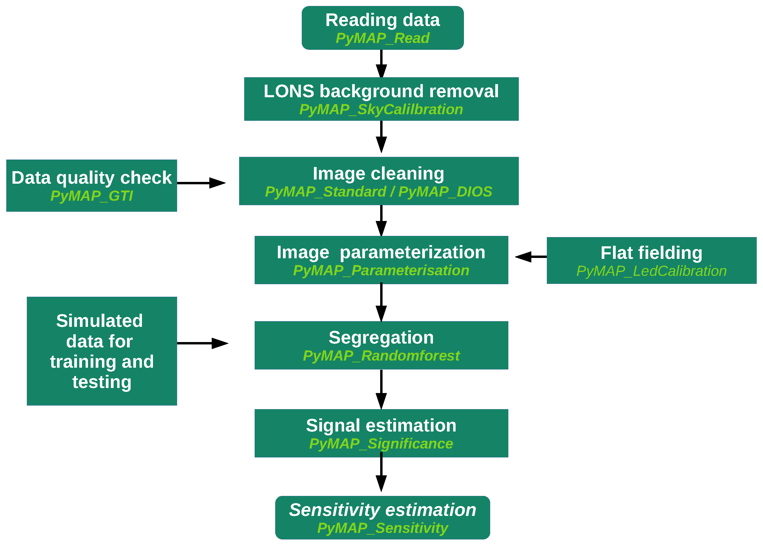
3. Python-Based MACE Data Analysis Package (PyMAP)

IACTs employ various pipelines tailored to specific telescopes, such as ctapipe [28] for Cherenkov Telescope Array Observatory (CTAO), MAGIC uses MARS [29], VERITAS utilizes both VEGAS [30] and EventDisplay [31], and the H.E.S.S telescope uses standard analysis [2] for CT-1 to CT-4 and Monoscopic Analysis Chains [32] for CT-5. PyMAP, a Python-based MACE data analysis package, is developed to extract gamma ray signals from a huge cosmic ray background, facilitating the study of various astrophysical sources. This package incorporates image cleaning techniques that extract the information by studying an EAS produced in IACT. The package is equipped with advanced classification technique, such as random forest for gamma/hadron segregation and signal estimation. It also provides a platform for implementing and testing new image cleaning and classification algorithms. The details of the functions in PyMAP and their workings are elaborated below. An overview of dataflow inside the package is given in Appendix A in the form of a flowchart. Data recorded from the source direction are passed through various data quality checks and calibrations before they are selected for analysis.

3.1. Good Time Interval (GTI)

The data recorded by the telescope are not always of high quality; they can be affected by sudden fluctuations due to electronic noise or abrupt increases in background light level. A GTI utility “PyMAP_GTI.py” helps to remove bad quality data based on various important parameters, such as if 5% of the total pixels in the trigger region have a value of average Single Channel Rate (SCR) that is out of bounds by two standard deviations of their respective values, an event is rejected. If one-third of the channels are dead due to the local light source reaching near the observatory, then the event is discarded. Also, if the Prompt Coincidence Rate (PCR), also called the trigger rate of the telescope, is out of bounds by 10 % due to some stray light, those events are rejected. The time interval left after these checks is considered to be a GTI. The profile analysis utility is crucial for event selection. It operates by examining the integrated peak profile of an event; if the value falls outside a window of 32 ns, the event is discarded.

3.2. Reading the Data
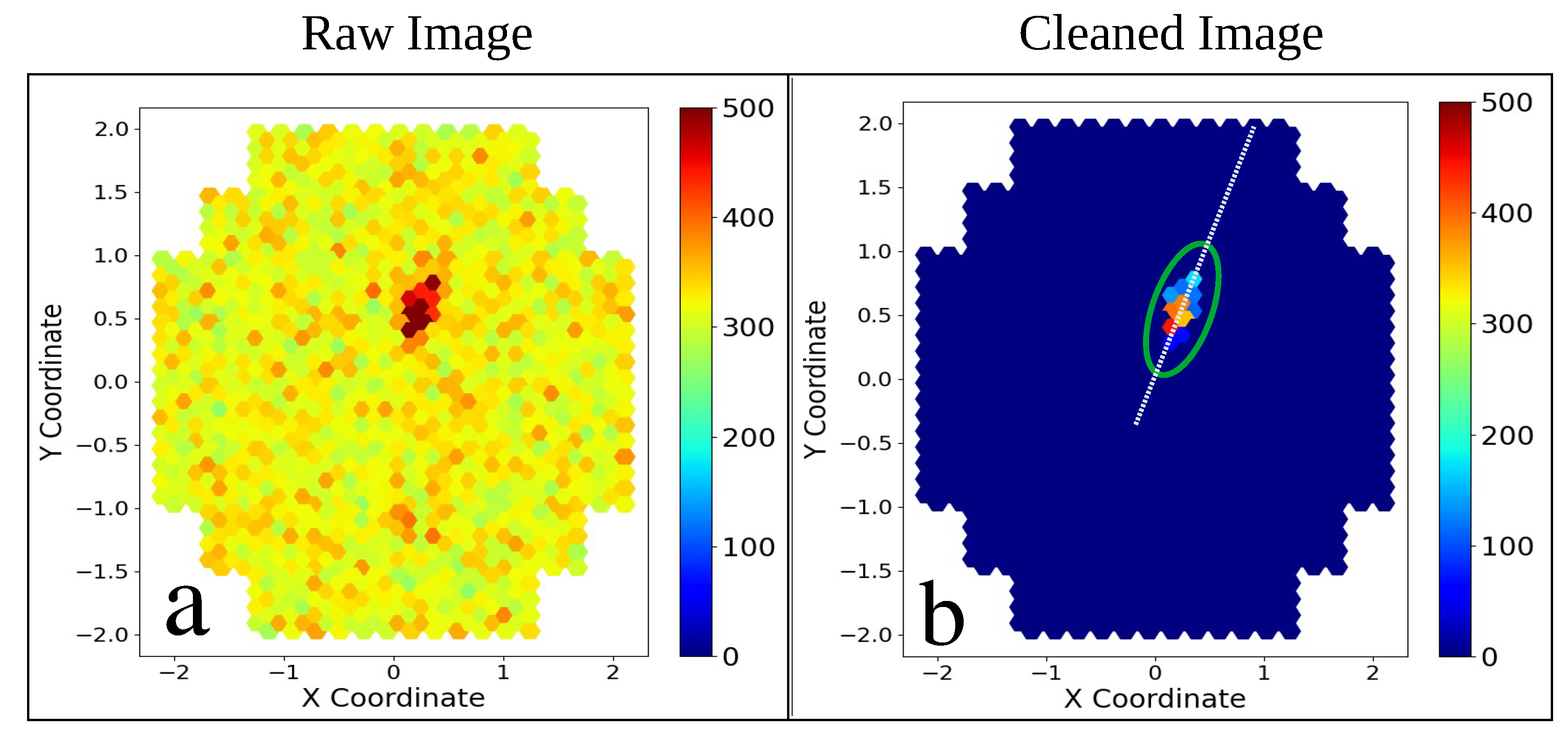
“PyMAP_ImageCleaning.py” utility includes function “PyMAP_Read”, which is used to read the recorded data for analysis. It converts the recorded data to the ROOT format for efficient organization and retrieval of large datasets. PyROOT libraries are implemented that leverage advanced C++ features within Python, allowing the utilization of C++ classes and interaction with libraries using Python syntax. The features of PyROOT software are also incorporated into data analysis, including data processing, data utilization, plot generation, and output writing.

3.3. Image Cleaning

The good quality data are now fed into an image cleaning utility, which includes various functions. Firstly, for sky and LED calibration, a fundamental requirement during observations is to conduct them during moonless nights to minimize the background caused by the moonlight. To further reduce background noise, it is important to account for the NSB. The photon flux due to NSB at the Hanle site is ∼ 10 12 ph m 2 s 1 sr 1 [20]. During observation, sky data are recorded every 1 min, which helps to remove background due to NSB. Another essential requirement for accurate signal estimation is to normalize the gain for all the PMTs used in the detector. To achieve this, an LED drive system is installed, which periodically flashes diffused LED light onto the detector. During each observation, LED data are recorded alongside sky data to monitor both changes in the sky and the health of the PMTs. The functions in this utility use the sky and LED integrated charge counts to estimate the mean and standard deviation (SD) for each PMT every time the sky and LED data are recorded. The sky mean of each pixel refers to the average light content due to NSB, and subtracting sky mean counts from total counts during observation for each PMT will lead to the removal of the NSB. This all is handled by “PyMAP_SkyCalibration”. Equation (1) explains the mathematics for the same. Gain normalization for each PMT is carried out using the “PyMAP_LedCalibration” function. In this, the mean and SD of LED counts estimated are used, and a reference pixel near the center of the camera is selected. The counts in the reference pixel are used to estimate the factor for the deviation in counts in all other PMTs. Factor estimation is given in Equation (2), where R r denotes the counts in the reference pixels and c l e a n C o u n t s i in the ith pixel. The counts in each PMT get updated as shown in Equation (3) concerning the reference pixel.
c l e a n C o u n t s i = t o t a l C o u n t s i s k y M e a n i
where i represents the pixel number.
F a c t o r i = R r c l e a n C o u n t s i
c l e a n C o u n t s U i = F a c t o r i c l e a n C o u n t s i

3.4. Standard Method Cleaning

The sky background removal is not enough to get a clean image of the EAS. Further image cleaning is a crucial step in IACTs. Several techniques have been developed by many IACTs to enhance the sensitivity and accuracy of the telescope’s ability to detect faint gamma ray signals. One of the most commonly used method is two-level thresholding, also referred to as tail-cut cleaning [33]. Wavelet-based cleaning has been implemented in the Whipple telescope [34]. Other techniques implemented are the island method [35], the two-level filter technique [2], and the next nearest neighbor cleaning method [36]. MACE data analysis employs threshold-based cleaning, commonly referred to as standard cleaning. “PyMAP_StandardCleaning” function in the PyMAP package incorporates the standard image cleaning technique. This technique implements thresholds to remove stray pixels or spurious images from an event. In the standard image cleaning method, we have implemented two threshold values, Picture threshold (PT) = 6.5 and Boundary threshold (BT) = 2.6 . This technique is applied in three steps. Firstly, BT value discards all the pixels that do not meet the criteria in Equation (4). Secondly, PT pixels are marked based on the criteria given in Equation (5). In the second step, all the pixels retained from the first step are re-examined. If any pixel does not have at least one PT pixel within its boundary, its count is set to zero. Thirdly, any standalone pixel remaining after the previous steps is considered a stray pixel if its count is less than 10 × s t d e v . Such pixels are discarded. This is how a cleaned image of the EAS is retained in the camera plane of the telescope.
c l e a n C o u n t s U k > B T × s t d e v ( s k y C o u n t s k )
c l e a n C o u n t s U i > P T × s t d e v ( s k y C o u n t s i )

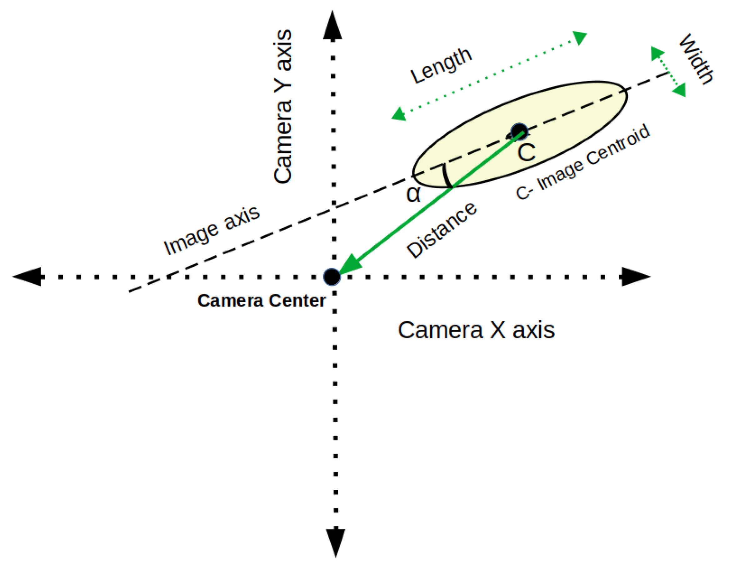
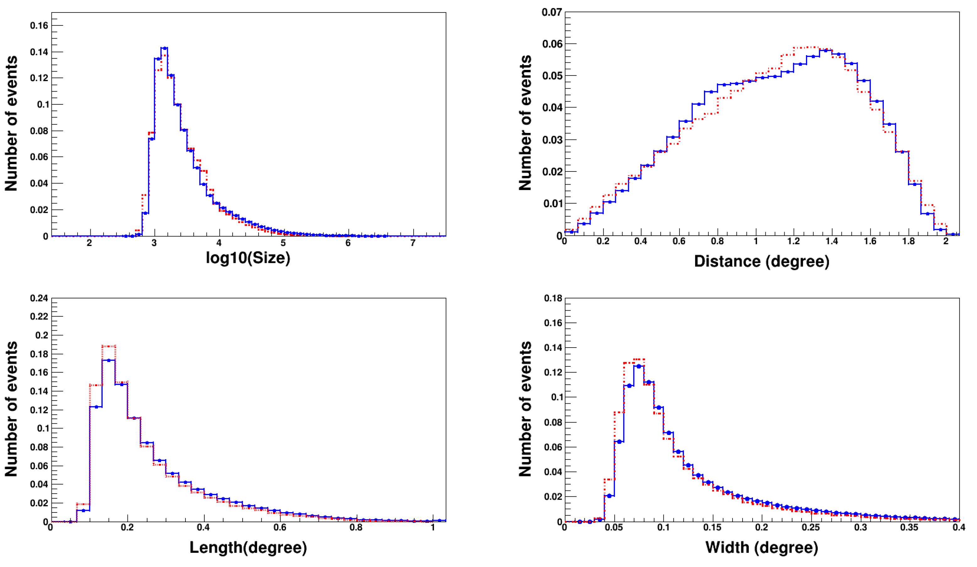
3.5. Image Parameterization

Image parameterization extracts quantitative features from Cherenkov images, enabling the differentiation of gamma rays from cosmic ray backgrounds. The Hillas Parameters represent key features of an EAS image on the camera plane (Figure 1). Derived by Hillas [23], include size, width, length, distance, alpha ( α ), leakage, etc. The representation of Hillas parameters for an image of an EAS on the camera plane is given in Figure 1. “PyMAP_ImageParameters” function in the PyMAP package incorporates the Hillas technique to calculate these parameters. The segregation is possible due to the difference in the interaction of gamma rays and cosmic rays with the atmospheric nuclei [24]. Figure 2a represents a simulated [37] EAS image on the camera plane, which includes background fluctuations due to the night sky. Figure 2b is the cleaned image on which the Hillas technique is applied. This 2D image of the EAS formed on the camera plane captures crucial information about the EAS development and the source location. In this study, a subset of observation data, approximately 120 min, from the Crab Nebula source within a zenith angle range of 10 20 has been analyzed. This dataset represents a portion of the observations used in this study and is derived from previously published results obtained by the MACE telescope [37]. After implementing the GTI utility (“PyMAP_GTI.py”), the data retained are around 95 min. The Hillas parameters estimation is done for the retained data, using the “PyMAP_ImageParameters” utility of the PyMAP package. The PyMAP package includes dedicated functions for the segregation technique, such as “PyMAP_Randomforest” implemented for gamma/hadrons segregation and signal estimation, described in the Section 3.6.

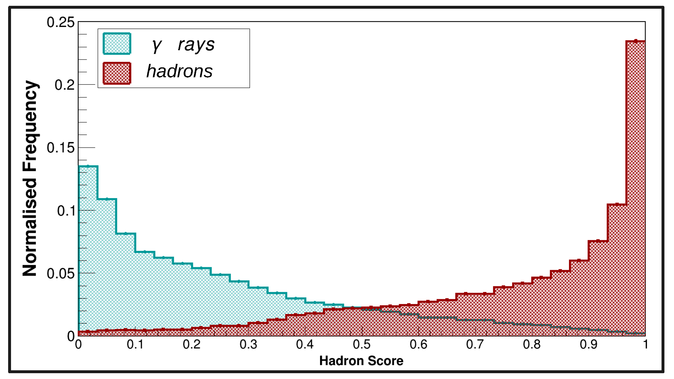
3.6. Image Classification Using Random Forest

The Random Forest algorithm [38] is a powerful machine learning technique widely used for high-accuracy classification tasks. It operates as an ensemble of decision trees, each utilizing input features such as Hillas parameters for data classification. The effectiveness of the model heavily relies on optimizing these input features. The hscore, a critical output of the model, quantifies the probability of an event being classified as a cosmic ray. In Figure 3, the green and red distributions represent the hscore for simulated gamma ray and cosmic ray events, respectively. A function of hscore as a function of the incoming particle’s energy is derived and subsequently applied to the observed data for signal estimation. This optimization enhances the ability of the hscore to effectively discriminate between gamma rays and cosmic rays. The feature importance values for all input features used to train the Random Forest classifier are presented in Figure 4. These values highlight the parameters that have the greatest influence on distinguishing gamma rays from the cosmic ray background, providing valuable insights into the model’s decision-making process.
We have optimized the hscore cut value independently for the image cleaning method. To optimize the cut, we have considered simulated data and divided them into three energy bins, E < 80 GeV, 80 GeV ≤ E ≤ 300 GeV and E > 300 GeV. To obtain the significance we have applied the optimized hscore values, and the signal region was considered up to 25° in the alpha plot. The simulated data sample used for the cut optimization include 2 × 10 5 events for the gamma ray and 1.5 × 10 5 for the hadrons. A total of 70% of events are used for training, and 30% of events are used for testing. After optimization, we applied these cuts on the observational data recorded for the Crab nebula source direction. The observed excess gamma ray events are 1230 ± 106, with a statistical significance [39] of 11.6 σ for the standard image cleaning method. The following sub-sections are dedicated to the implementation of a new image cleaning technique, DIOS, its workings, and its importance. We have employed the random forest segregation technique on the DIOS method, which was then compared with the standard image cleaning.

3.7. DIOS Image Cleaning Method

A new image cleaning method is developed to effectively remove the noise from the EAS images captured on the camera plane. This enhanced cleaning technique improves the retention rate of the events, resulting in a higher percentage of events for analysis. In the DIOS method, an image goes through several cleaning steps before it can be parameterized. First, the background noise due to NSB is removed using Equation (1). Next, only those pixels are retained if their charge content is greater than a certain threshold as shown in Equation (6), where c o u n t s k refers to the charge count in the kth pixel and s t d e v ( s k y C o u n t s k ) refers to the deviation in the kth pixel. The value of D is optimized using simulation data, and the resulting optimal value is found to be 2.4, as lowering the threshold further leads to the retention of dummy pixels, affecting the proper image retention.
c l e a n C o u n t s U k > D × s t d e v ( s k y C o u n t s k )
The next step is very crucial and helps to retain the pixels that are part of the image cluster. A schematic of DIOS working is given in Figure 5, where the orange color represents the pixel under “consideration”, blue color pixels are not yet checked, green color is “ok” pixels (it will be a part of an image). Red color flag pixels will be removed from an image at the end of image cleaning. In this algorithm, two steps (Step 1 and Step 2) are applied. In Step 1, the algorithm checks whether the pixel under consideration(orange) has minimum two adjacent pixels. Based on this check, two conditions arise: “yes” or “no”. If the condition is “yes”, the pixel is marked as an “ok pixel” (green) and no need to go to Step 2, as shown in Scenario 1.
If the condition is “no”, it means pixel (orange) has only one adjacent nearby pixel and Step 2 is applied as shown in Scenario 2. In this step, the pixel (orange) asks for checking a minimum of two nearby pixels (excluding itself) around the adjacent pixel. Based on the pixel number 4 location, two arrangements are possible, as shown in CASE-A and CASE-B. Let pixel 1 be under consideration (orange); it has only one adjacent pixel (pixel 2), so Step 2 is applied. In Step 2, the algorithm checks the adjacent pixels of pixel 2 to determine whether pixel 1 should be included in the image. If pixel 2 has a minimum of two adjacent pixels (excluding pixel 1), then pixel 1 is now tagged as an “ok pixel” (green) (CASE-B). Otherwise, it is marked as a rejected pixel (red) that is considered for removal (CASE-A) at the end of the image cleaning procedure. Similarly, all the other pixels in CASE-A and CASE-B are checked; pixels that are tagged as “ok pixels” (green) are included as part of the image, while those marked as red color are excluded in the output cleaned image.
The third step, which is the final stage of an event cleaning, removes the dummy images from an actual image. Even though the image is reconstructed, due to the lower threshold applied, there remains a possibility of retaining dummy clusters along with an actual image cluster. To remove those, we calculate the Signal/Noise (S/N) value for each cluster retained, and a cluster having a high S/N is selected as an actual image of the shower. This way, we can remove the dummy clusters retained due to fluctuations.

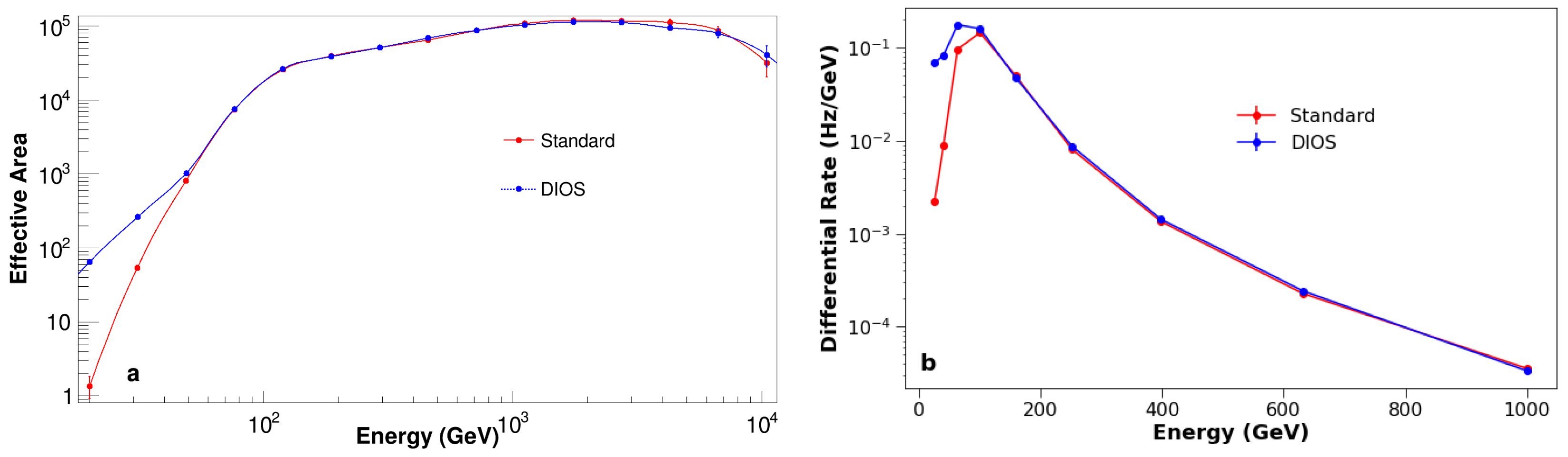
3.8. Importance of DIOS Image Cleaning Method

A comparative study is done between the DIOS and the standard image cleaning technique to quantify the performance of the DIOS image cleaning method. Initially, both DIOS and standard image cleaning methods are applied to simulated image data to compare the percentage of the retained events. The DIOS image cleaning method retains around 93% of the events, and the Standard method retains around 76% of the total events. The DIOS method is capable of retaining 17% more events than the standard method, reflecting a better performance of the DIOS image cleaning method. The DIOS method not only retains more events but is also effective in retaining a proper image of an incoming event in the camera plane. To check the bias in the new image cleaning method, we have considered a sample of 50,000 events of sky data, and it was observed that both image cleaning techniques are able to reject all the sky events. Figure 6 presents an example of a simulated gamma ray image on the camera plane where (a) represents an image after sky background removal, (b) is a cleaned image using standard cleaning, and (c) is the cleaned image using the DIOS cleaning method. Figure 6b demonstrates that the image generated using the standard cleaning method gets truncated as the hard cleaning thresholds are applied. In contrast, the DIOS image cleaning method produces a complete and properly formed image, which generally happens with the low-energy or fainter images of incoming gamma rays.
The Alpha distribution of all simulated gamma rays and cosmic ray background events using two different image cleaning methods after applying cuts is shown in Figure 7. It illustrates that a larger number of gamma ray events are retained in the DIOS method as compared to the standard method. The DIOS alpha distribution shows broadening; this is due to the retention of low-energy gamma ray events [40]. To evaluate the DIOS method, the observation data from the Crab Nebula source direction and their off-source direction are considered for this study. To begin with the detailed performance, firstly, the Hillas parameters distribution obtained from observation data using the DIOS method is compared with the parameters obtained using simulated cosmic ray images. We observe a satisfactory agreement between the simulated and the measured parameters as shown in Figure 8. However, a slight variation is observed, which can be attributed to the fact that the simulated data include contributions from protons, while the observational data account for contributions from other cosmic ray particles as well.
The effective gamma/hadron classification in this study is achieved through the implementation of a Random Forest classifier. In the context of the newly proposed image cleaning method, we apply this gamma/hadron segregation technique to generate the alpha distribution for observation data. The optimized hscore cut is applied to both the standard image cleaning method and the DIOS method to ensure a consistent basis for comparison. By maintaining an identical hscore threshold across both cleaning techniques, we can directly evaluate their relative performance in terms of event classification and image quality. Alpha Distribution for the DIOS image cleaning method gives the statistical significance of 14.5 σ with an excess of 1921 ± 133 gamma ray event. Obtained results are given in Table 1 and it signify the better performance of the DIOS method over the standard method. The statistical significance increases from 11.6 σ to 14.5 σ with an excess of 691 gamma ray events.
The Alpha distribution obtained using the “PyMAP_Significance.py” utility is given in Figure 9; the green region represents the distribution obtained from the source and blue is from the off data. The ON-OFF data analysis procedure is followed, which helps to estimate gamma-like events that are not gamma but instead cosmic ray background events. The excess number of gamma ray events is estimated by subtracting the total number of events in the blue region from the total number of events in the green region up to 25 degrees.

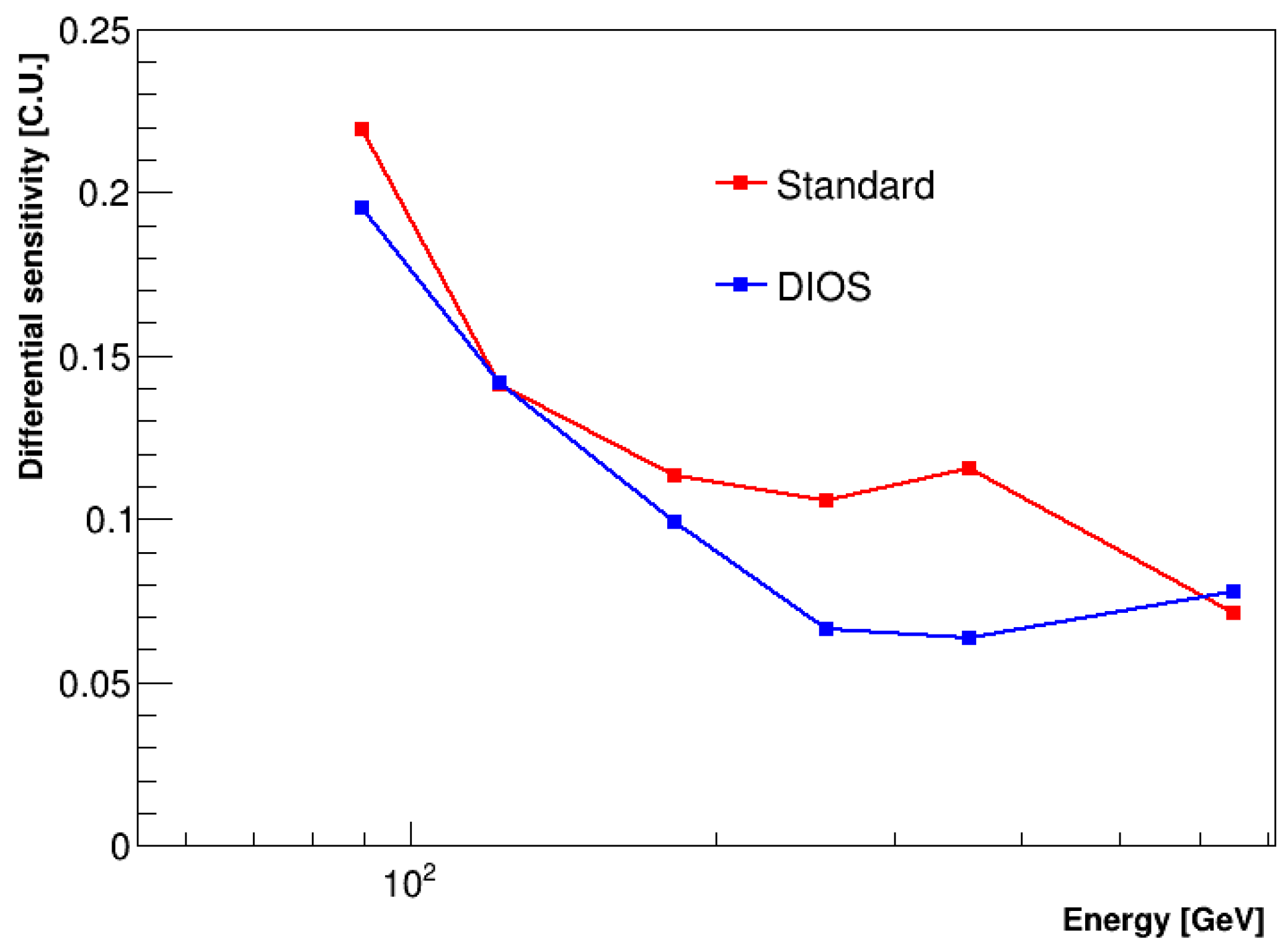
4. Sensitivity Estimation

To conclusively demonstrate that the DIOS method outperforms the existing approach, it is essential to quantify its performance. The integral flux sensitivity obtained with a 5 σ significance level in 50 h of observation is around 9.8% [37] and 7% of Crab units for the standard and DIOS image cleaning methods, respectively. The difference in the integral sensitivity achieved is around 25%; this leads to an increase in the sensitivity of the MACE telescope with the implementation of the DIOS method. Figure 10a is the comparison plot of effective area, which illustrates the greater retention of gamma ray events in lower energy using the DIOS image cleaning method. Figure 10b is the differential rate curves for gamma rays using DIOS and standard cleaning method.
d N γ d E = 2.79 × 10 10 E 1 T e V 2.59 m 2 s 1 GeV 1
To evaluate the performance of the DIOS image cleaning method, we have obtained the differential sensitivity curve (5 bins per decade) in Crab Units and compared it with the standard cleaning method. A comparison for both the cleaning method is shown in Figure 11. For DIOS method it is observed that the improvement is actually at the energies of a few hundred GeV and at lower energy. The extra pixels are retained by DIOS that help in better reconstruction of the shower, thus enhancing the sensitivity.

5. Conclusions

In this research work, we have developed the MACE data analysis package named PyMAP, which incorporates the python and machine learning libraries to study VHE gamma ray sources observed by the MACE telescope. We have used the Hillas parameterization technique to find the nature of the recorded image of the EAS. In this, we have discussed the importance of all the functions and utilities developed in the PyMAP package. The PyMAP package includes a function for the signal estimation that is a random forest segregation technique. We discuss the importance of the new image cleaning method DIOS. Further, we use the random forest segregation technique in a new image cleaning method, DIOS, to study its performance. This method is developed to improve the sensitivity of the MACE telescope. It is observed that the DIOS method performs better when compared to the standard image cleaning approach, effectively enhancing the signal-to-noise ratio, achieving a lower energy threshold, and increasing the number of gamma ray events retained, thereby improving the sensitivity. By more precisely filtering out background noise and preserving relevant features, this method provides clearer, more reliable data, which is critical for advancing our understanding of VHE gamma ray sources. The results highlight the potential of this approach to improve observational sensitivity in ground-based gamma-ray astronomy, making it a valuable tool for future research. The sensitivity of the DIOS image cleaning method could be further enhanced by exploring various machine learning and AI tools, though this is beyond the scope of the present work. Future investigations into these advanced techniques may offer additional improvements in background suppression and signal clarity, potentially leading to even more accurate detection capabilities in gamma ray astronomy.

Author Contributions

Package Development, M.K. and P.C.; methodology, M.K. and P.C.; validation, M.K., P.C., A.P. and C.B.; formal analysis, M.K., P.C. and A.P.; investigation, M.K. and P.C.; resources, M.K., P.C. and C.B.; data curation, M.K., P.C., A.P. and C.B.; writing—original draft preparation, M.K., P.C. and A.P.; writing—review and editing, P.C., C.B., K.K.S. and K.K.Y.; visualization, P.C., K.K.S., C.B. and K.K.Y.; supervision, K.K.Y. All authors have read and agreed to the published version of the manuscript.

Funding

This research received no external funding.

Data Availability Statement

The data presented in this study are available on reasonable request to the corresponding authors.

Acknowledgments

The authors sincerely express their profound gratitude to the anonymous reviewers for their critical and insightful comments and suggestions which have undeniably played a pivotal role in the overall improvement of the manuscript. We extend our sincere gratitude to the contributions made by the MACE observation team at Hanle, Ladakh, our Simulation team, colleagues from the Electronics Division, Control and Instrumentation Division, Center for Design and Manufacture, and Computer Division at BARC for their dedicated involvements in the various sub-systems of the MACE telescope.

Conflicts of Interest

The authors declare that they have no known competing financial interests or personal relationships that could have appeared to influence the work reported in this paper.

Abbreviations

The following abbreviations are used in this manuscript:
VHEVery High Energy
MACEMajor Atmospheric Cherenkov Experiment
PyMAPPython-based MACE Analysis Package
IACTImaging Atmospheric Cherenkov Telescope
DIOSDenoising Image of Shower
NSBLight Of Night Sky
EASExtensive Air Shower
PMTPhoto Multiplier Tube
DASData Aquisition Systems
GTIGood Time Interval
LEDLight Emitting Diode
SCRSingle Channel Rate
SDStandard Deviation
BTBoundary Threshold
PTPicture Threshold
RFRandom Forest

Appendix A

Figure A1. Dataflow of various utilities in PyMAP. Light green italic represents the concerned utility name under PyMAP.
Galaxies 13 00014 g0a1

References

  1. Hess, V.F. Über beobachtungen der durchdringenden Strahlung bei sieben Freiballonfarten. Phys. J. 1912, 13, 1086–1091. [Google Scholar]
  2. Aharonian, F.; Akhperjanian, A.G.; Bazer-Bachi, A.R.; Beilicke, M.; Benbow, W.; Berge, D.; Bernlöhr, K.; Boisson, C.; Bolz, O.; Borrel, V.; et al. Observations of the Crab nebula with HESS. Astron. Astrophys. 2006, 457, 899–915. [Google Scholar] [CrossRef]
  3. Cortina, J. Status and First Results of the MAGIC Telescope. Astrophys. Space Sci. 2005, 297, 245–255. [Google Scholar] [CrossRef]
  4. Hanna, D.; Acciari, V.A.; Amini, R.; Badran, H.M.; Blaylock, G.; Bradbury, S.M.; Buckley, J.H.; Bugaev, V.; Butt, Y.; Byrum, K.L.; et al. First results from VERITAS. Nucl. Instruments Methods Phys. Res. Sect. A Accel. Spectrometers, Detect. Assoc. Equip. 2008, 588, 26–32. [Google Scholar] [CrossRef]
  5. Meyer, M.; Horns, D.; Zechlin, H.S. The Crab Nebula as a standard candle in very high-energy astrophysics. Astron. Astrophys. 2010, 523, A2. [Google Scholar] [CrossRef]
  6. Tickoo, A.K.; Koul, R.; Rannot, R.C.; Yadav, K.K.; Chandra, P.; Dhar, V.K.; Koul, M.K.; Kothari, M.; Agarwal, N.K.; Goyal, A. Long term performance evaluation of the TACTIC imaging telescope using 400 h Crab Nebula observation during 2003–2010. Pramana 2014, 82, 585–605. [Google Scholar] [CrossRef]
  7. Weekes, T.C.; Cawley, M.F.; Fegan, D.J.; Gibbs, K.G.; Hillas, A.M.; Kowk, P.W.; Lamb, R.C.; Lewis, D.A.; Macomb, D.J.; Porter, N.A.; et al. Observation of TeV Gamma Rays from the Crab Nebula Using the Atmospheric Cerenkov Imaging Technique. Astrophys. J. 1989, 342, 379–392. [Google Scholar] [CrossRef]
  8. Abe, H.; Abe, K.; Abe, S.; Aguasca-Cabot, A.; Agudo, I.; Crespo, N.A.; Antonelli, L.A.; Aramo, C.; Arbet-Engels, A.; Arcaro, C.; et al. Observations of the Crab Nebula and Pulsar with the Large-Sized Telescope Prototype of the Cherenkov Telescope Array. Astrophys. J. 2023, 956, 80. [Google Scholar] [CrossRef]
  9. Nishimura, J.; Kamata, K. On Theory of cascade Showers. Prog. Theor. Phys. 1952, 7, 185–192. [Google Scholar] [CrossRef]
  10. Weekes, T.C. Very High Energy Gamma-ray Astronomy; Institute of Physics Publishing: Bristol, UK, 2003; Volume 3, pp. 43–44. [Google Scholar]
  11. Maier, G. Cosmic-ray events as background in imaging atmospheric Cherenkov telescopes. Astropart. Phys. 2007, 28, 72–81. [Google Scholar] [CrossRef]
  12. Sobczynska, D. Natural limit on the gamma/hadron separation for a stand alone air Cherenkov telescope. J. Phys. G Nucl. Part. Phys. 2007, 35, 2279–2288. [Google Scholar] [CrossRef]
  13. Krennrich, F. New generation atmospheric Cherenkov detectors. Astropart. Phys. 1999, 11, 235–242. [Google Scholar] [CrossRef]
  14. Krennrich, F. The Next Generation of Ground-based Gamma Ray Telescopes. Am. Phys. Soc. 2001, 46, 2. [Google Scholar]
  15. Heck, D.; Knapp, J.; Capdevielle, J.N.; Schatz, G.; Thouw, T. Corsika: A Monte Carlo Code to Simulate Extensive Air Showers; Technical Report, Kernforschungszentrum Karlsruhe, 51.02.03; LK 01; Wissenschaftliche Berichte, FZKA-6019. 1998. Available online: https://digbib.bibliothek.kit.edu/volltexte/fzk/6019/6019.pdf (accessed on 23 September 2019).
  16. Cawley, M.F. Development of the atmospheric Cherenkov imaging technique. Il Nuovo Cimento C 1996, 19, 959–963. [Google Scholar] [CrossRef]
  17. Weekes, T.C. The Atmospheric Cherenkov Imaging Technique for Very High Energy Gamma-ray Astronomy. arXiv 2005, arXiv:astro-ph/0508253. [Google Scholar]
  18. Mirzoyan, R. Technological Novelties of Ground-Based Very High Energy Gamma-Ray Astrophysics with the Imaging Atmospheric Cherenkov Telescopes. Universe 2024, 8, 219. [Google Scholar] [CrossRef]
  19. Hillas, A.M. Differences between gamma-ray and hadronic showers. Space Sci. Rev. 1996, 75, 17–30. [Google Scholar] [CrossRef]
  20. Khurana, M.; Singh, K.K.; Godiyal, S.; Yadav, K.K. Effects of the moonlight on the operating parameters of the MACE gamma ray telescope: A feasibility study. J. Astrophys. Astron. 2022, 43, 12. [Google Scholar] [CrossRef]
  21. Hinton, J.A. The Status of TeV Gamma-Ray Astronomy. New J. Phys. 2009, 11, 055005. [Google Scholar] [CrossRef]
  22. Aharonian, F.A. Very High Energy Cosmic Gamma Radiation: A Crucial Window on the Extreme Universe; World Scientific Publishing: Singapore, 2008; ISBN 978-981-256-355-8. [Google Scholar]
  23. Hillas, A.M. Cerenkov light images of EAS produced by primary gamma rays and by hadrons. In Proceedings of the 19th International Cosmic Ray Conference (ICRC 1985), San Diego, CA, USA, 11–23 August 1985; Volume 3, pp. 445–448. [Google Scholar]
  24. Hillas, A.M. Angular and energy distribution of charged particles in electron-photon cascades in air. J. Phys. G Nucl. Phys. 1982, 8, 1461–1473. [Google Scholar] [CrossRef]
  25. Srivastava, S.; Jain, A.; Nair, P.M.; Sridharan, P. MACE camera controller embedded software: Redesign for robustness and maintainability. Astron. Comput. 2020, 30, 123–135. [Google Scholar] [CrossRef]
  26. Jain, A.; Srivastava, S.; Mahesh, P.; Deshpande, J.; Padmini, S. Autonomous observation, control, data acquisition and monitoring of MACE telescope. Astropart. Phys. 2024, 157, 102922. [Google Scholar] [CrossRef]
  27. Yadav, K.K.; Chouhan, N.; Thubstan, R.; Norlha, S.; Hariharan, J.; Borwankar, C.; Chandra, P.; Dhar, V.K.; Mankuzhyil, N.; Godambe, S.; et al. Commissioning of the MACE gamma-ray telescope at Hanle, Ladakh, India. Curr. Sci. 2022, 123, 1428–1435. [Google Scholar] [CrossRef]
  28. Linhoff, M.; Bhattacharyya, S.; Pérez Romero, J.; Stanič, S.; Vodeb, V.; Vorobiov, S.; Zavrtanik, D.; Zavrtanik, M.; Živec, M. ctapipe-Prototype Open Event Reconstruction Pipeline for the Cherenkov Telescope Array. In Proceedings of the 38th International Cosmic Ray Conference, ICRC (2023), Nagoya, Japan, 26 July–3 August 2023; Volume 444, p. 703. [Google Scholar]
  29. Moralejo, A.; Gaug, M.; Carmona, E.; Colin, P.; Delgado, C.; Lombardi, S.; Mazin, D.; Scalzotto, V.; Sitarek, J.; Tescaro, D. MARS, the MAGIC Analysis and Reconstruction Software. In Proceedings of the 31st International Cosmic Ray Conference (ICRC 2009), Lodz, Poland, 7–15 July 2009. [Google Scholar]
  30. Cogan, P. VEGAS, the VERITAS Gamma-ray Analysis Suite. arXiv 2007, arXiv:0709.4233. [Google Scholar]
  31. Maier, G.; Holder, J. Eventdisplay: An Analysis and Reconstruction Package for Ground-based Gamma-ray Astronomy. In Proceedings of the 35th International Cosmic Ray Conference (ICRC 2017), Busan, Republic of Korea, 12–20 July 2017. [Google Scholar]
  32. Holler, M.; Balzer, A.; Becherini, Y.; Klepser, S.; Murach, T.; de Naurois, M.; Parsons, R. Status of the Monoscopic Analysis Chains for H.E.S.S. II. In Proceedings of the 35th International Cosmic Ray Conference (ICRC 2013), Rio de Janeiro, Brazil, 2–9 July 2013. [Google Scholar]
  33. Konopelko, A. et al. [HEGRA Collaboration]. Detection of gamma-rays above 1-TeV from the Crab Nebula by the second HEGRA imaging atmospheric Cherenkov telescope at La Palma. Astropart. Phys. 1996, 4, 199–215. [Google Scholar] [CrossRef]
  34. Lessard, R.W.; Cayón, L.; Sembroski, G.H.; Gaidos, J.A. Wavelet imaging cleaning method for atmospheric Cherenkov telescopes. Astropart. Phys. 2001, 17, 427–440. [Google Scholar] [CrossRef]
  35. Bond, I.H.; Hillas, A.M.; Bradbury, S.M. An island method of image cleaning for near threshold events from atmospheric Čerenkov telescopes. Astropart. Phys. 2003, 20, 311–321. [Google Scholar] [CrossRef]
  36. Kherlakian, M. Application of the optimised next neighbour image cleaning method to the VERITAS array. arXiv 2023, arXiv:2309.14839. [Google Scholar]
  37. Borwankar, C.; Sharma, M.; Hariharan, J.; Venugopal, K.; Godambe, S.; Mankuzhyil, N.; Chandra, P.; Khurana, M.; Pathania, A.; Chouhan, N.; et al. Observations of the Crab Nebula with MACE (Major Atmospheric Cherenkov Experiment). Astropart. Phys. 2024, 159, 102960. [Google Scholar]
  38. Breiman, L. Random Forests. Mach. Learn. 2001, 45, 5–32. [Google Scholar] [CrossRef]
  39. Li, T.-P.; Ma, Y.-Q. Analysis methods for results in gamma-ray astronomy. Astrophys. J. 1998, 272, 313–324. [Google Scholar] [CrossRef]
  40. Wagnera, R.M.; Lopezb, M.; Masea, K.; Domingo–Santamariac, E.; Goebela, F.; Flixc, J.; Majumdara, P.; Mazinb, D.; Moralejod, A.; Panequea, D.; et al. Observation of the Crab nebula with the MAGIC telescope. In Proceedings of the 29th International Cosmic Ray Conference Pune (ICRC 2005), Pune, India, 3–10 August 2005; Volume 4, pp. 163–166. [Google Scholar]
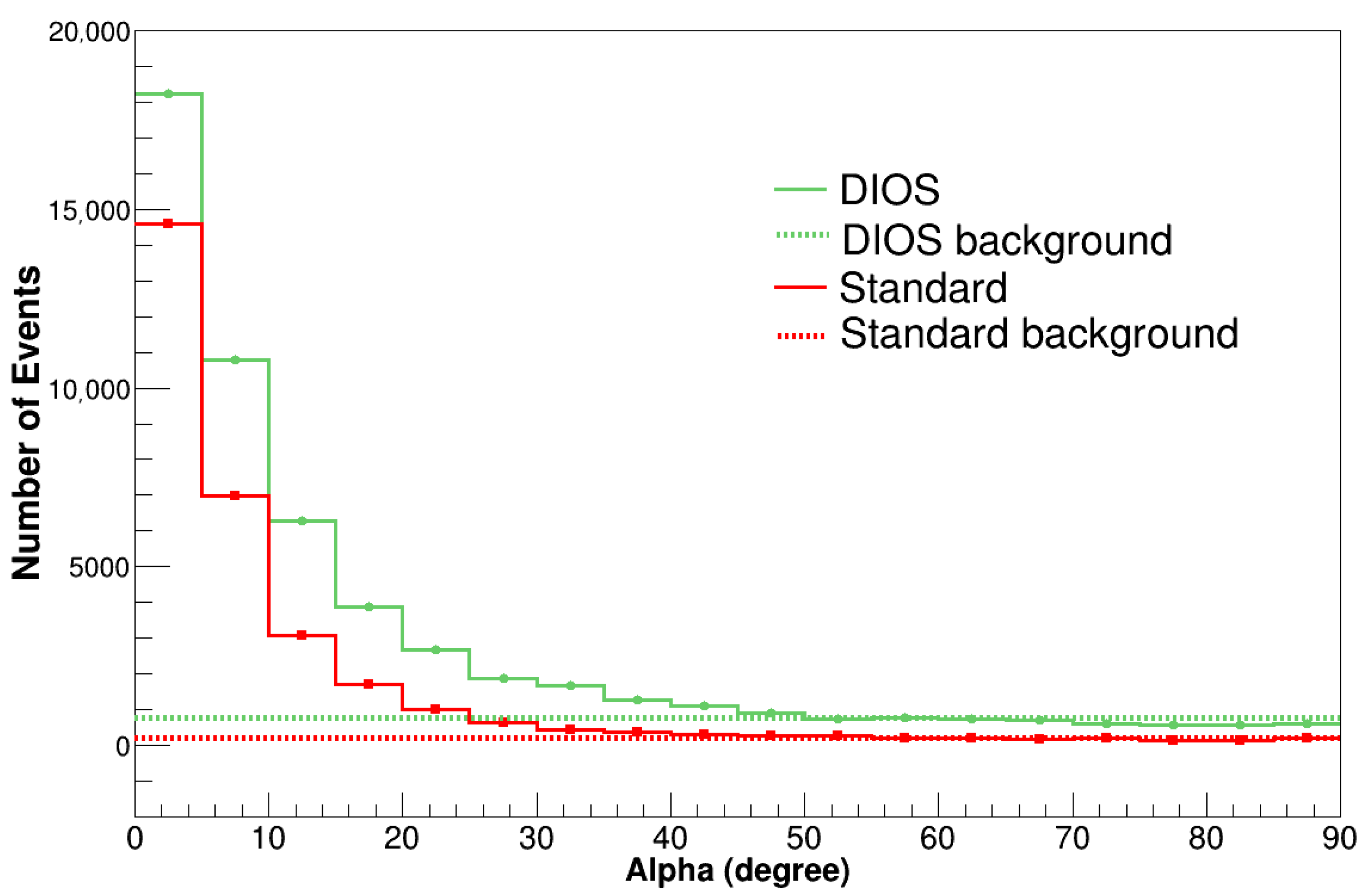
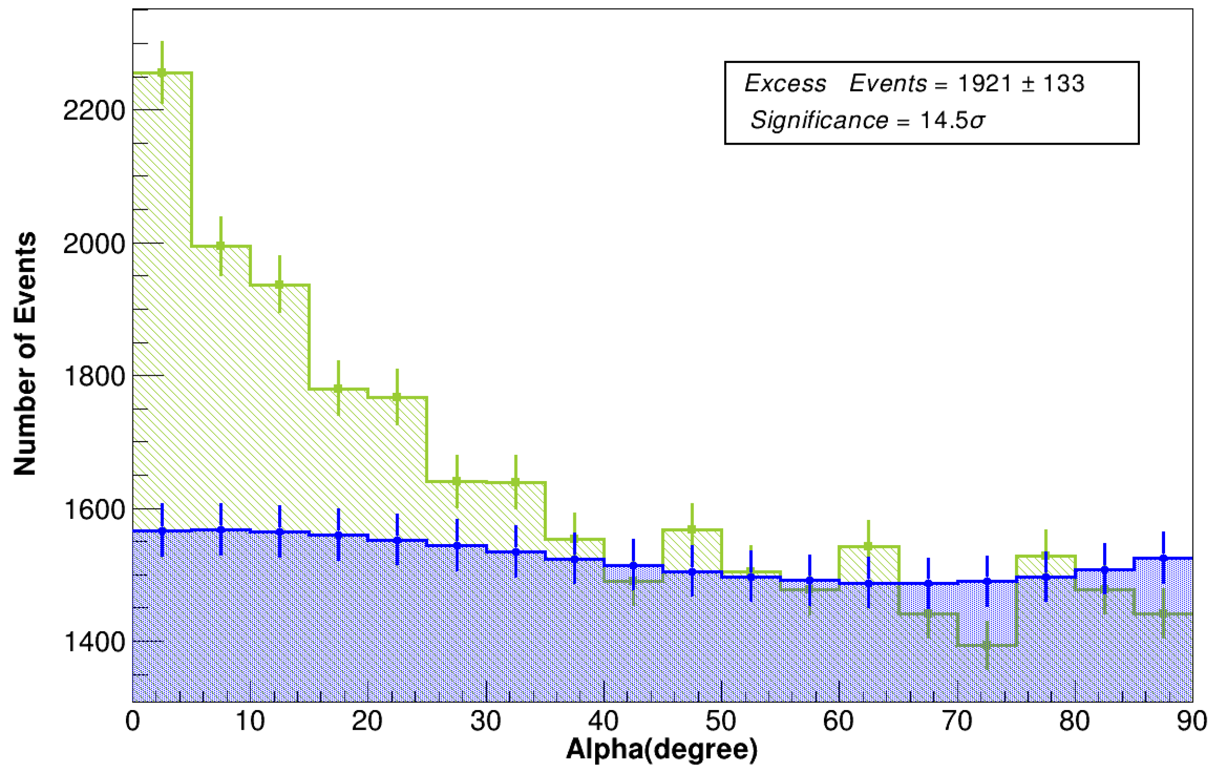
Figure 1. Representation of the Hillas Parameters on the camera plane.
Galaxies 13 00014 g001
Figure 2. (a) Raw simulated EAS image on the camera plane. (b) Cleaned image obtained after the implementation of image cleaning tools. The image extracted is parameterized using the Hillas parameterization technique.
Galaxies 13 00014 g002
Figure 3. The hscore distribution for γ and hadron events, green-shaded region represents hscore value for gamma like events and red for the cosmic ray events. The gamma rays were simulated with a differential energy spectrum given by d N / d E E 2.59 in the energy range of 10 GeV to 20 TeV, whereas the cosmic ray protons were simulated in the energy range of 20 GeV to 20 TeV with a spectral index of 2.7.
Galaxies 13 00014 g003
Figure 4. Pie chart showing feature importance of various Hillas parameters for gamma/hadron classification.
Galaxies 13 00014 g004
Figure 5. Working schematic for a new image cleaning method DIOS. Different scenarios and cases are illustrated to explain the procedure behind selecting pixels that are part of an image. The blue color pixel (not yet checked), orange colour pixel (under consideration), green is “ok pixels” (will be a part of the cleaned image), red pixels are “rejected pixels” (will not be a part of a cleaned image).
Galaxies 13 00014 g005
Figure 6. The given figure illustrates an example of a simulated gamma ray image in the camera plane where (a) represents an image after sky background removal, (b) is a cleaned image using standard cleaning, and (c) is a cleaned image using DIOS cleaning method.
Galaxies 13 00014 g006
Figure 7. Alpha distribution of all simulated gamma rays events (cuts applied) represented by solid line and cosmic ray background events (cuts applied) represented by dotted line, for two different image cleaning techniques. Different numbers of data samples are used for background and gamma rays. The green is for DIOS and red is for standard method. A total of 30% of total simulated events are used to generate the alpha distribution.
Galaxies 13 00014 g007
Figure 8. The normalized plots for the Hillas parameter distributions—log10 (size), distance, length, and width are shown. The blue distributions represent the observed off data, while the red distributions correspond to the simulated off data.
Galaxies 13 00014 g008
Figure 9. DIOS Alpha parameter distribution, the green-shaded region is from the Crab source direction and the blue-shaded region represents the background obtained from the Off region. Signal estimation is done using ON-OFF analysis. The signal region considered here is up to 25 degrees.
Galaxies 13 00014 g009
Figure 10. (a) Plot is the effective collection area of the MACE after applying two image cleaning methods. The red line is for standard cleaning and the blue is for the DIOS method. (b) Plot is the differential rate curves for gamma rays using DIOS and standard cleaning method. We have used a power law spectrum given in Equation (7). The two differential rates corresponding to power law spectrum of CRAB nebula peak at ∼80 GeV with the standard method and ∼60 GeV with the DIOS method.
Galaxies 13 00014 g010
Figure 11. The differential sensitivity plot for both image cleaning methods is expressed in Crab Units. The red solid line represents the standard method, while the blue line corresponds to the DIOS method.
Galaxies 13 00014 g011
Table 1. Comparison of excess gamma ray events, significance, and σ / T i m e ratio for two image cleaning methods, i.e., DIOS and standard cleaning. A total of 25% increase in the case of the DIOS method compared to the standard cleaning illustrates its better performance and improvement in sensitivity.
MethodExcess of Gamma Ray EventsSignificance σ / Time
DIOS1921 ± 13314.5 σ 1.49
Standard1230 ± 10611.6 σ 1.19
Disclaimer/Publisher’s Note: The statements, opinions and data contained in all publications are solely those of the individual author(s) and contributor(s) and not of MDPI and/or the editor(s). MDPI and/or the editor(s) disclaim responsibility for any injury to people or property resulting from any ideas, methods, instructions or products referred to in the content.

