
Simulations for the Locking and Alignment Strategy of the DRMI Configuration of the Advanced Virgo Plus Detector

 ,
,  , ,
, ,  and
and
Abstract
:1. Introduction
- Choice and characterization of the longitudinal and angular error signals used to control the DRMI Degrees Of Freedom (DOFs);
- Determination of suitable trigger signals used for the engagement of the control loops with the “coincidence lock” technique;
- Study of the behavior of the longitudinal control loops’ error signals when the DRMI mirrors are subject to misalignments.
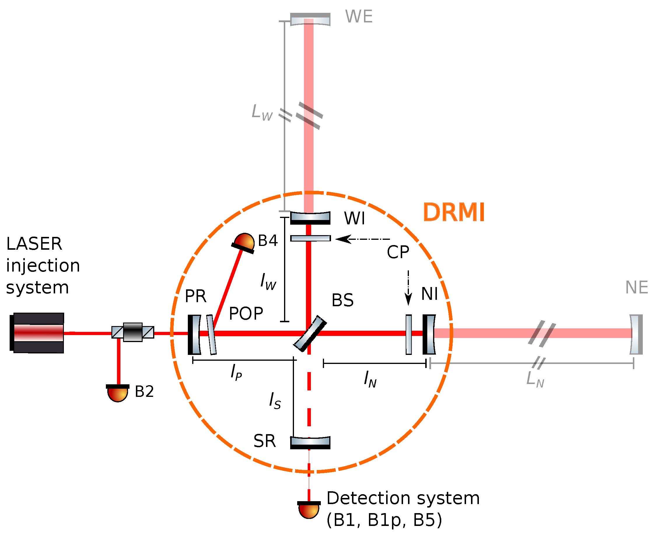
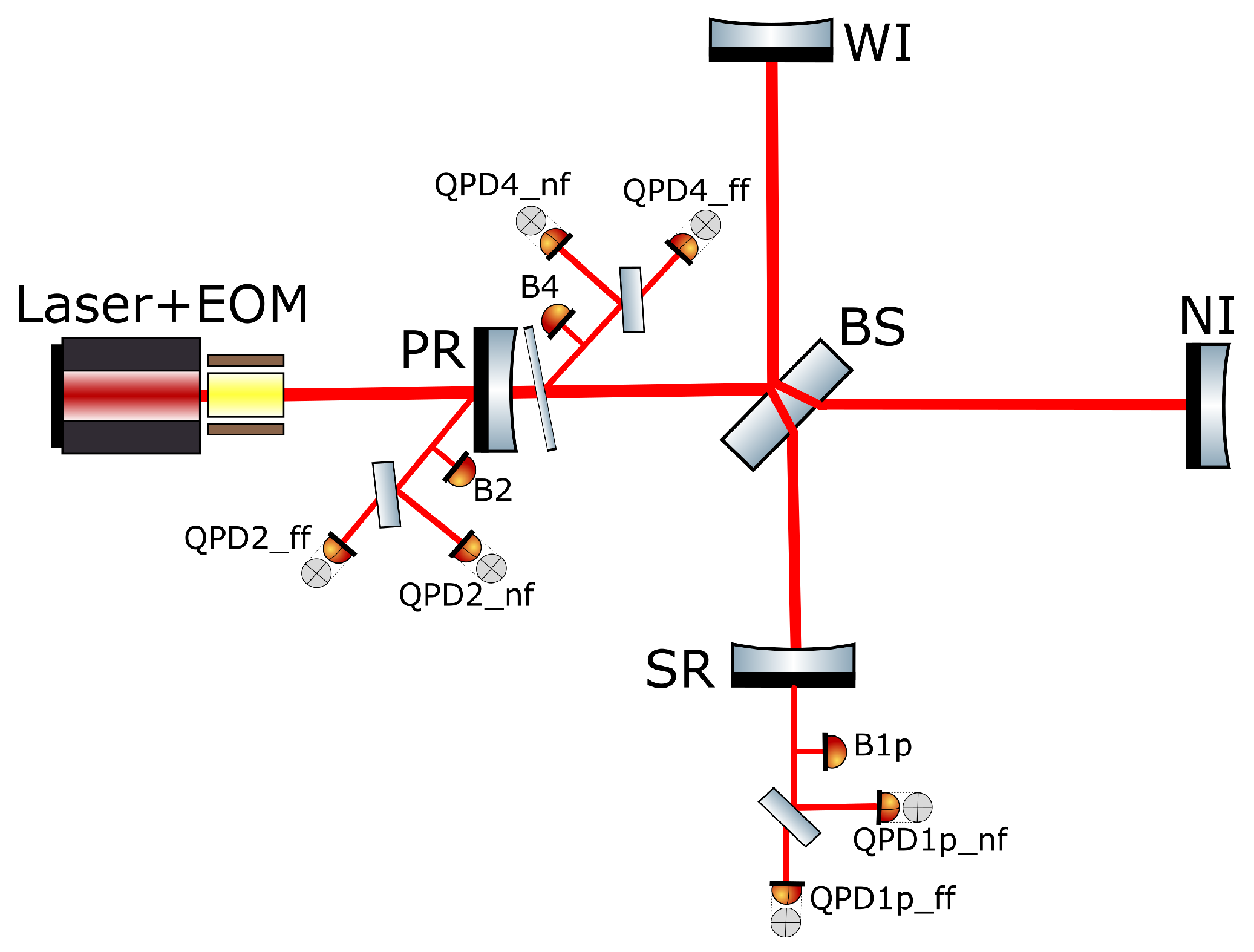
1.1. The DRMI Configuration
- MICH: the short Michelson needs to be in dark fringe, i.e., with a complete destructive interference;
- PRCL: the Power Recycling cavity needs to be resonant with the 6 MHz and the 56 MHz sidebands, and anti-resonant with respect to the Carrier (once the CARM offset reduction is complete and the arm Fabry-Pérot cavities become resonant, the Carrier will become resonant in the PR cavity too due to the change in the phase of the cavities’ reflected field);
- SRCL: the Signal Recycling cavity needs to be resonant with the 56 MHz sideband and resonant with respect to the Carrier (due to the same phase shift affecting the field in the PR cavity, at the end of the CARM offset reduction, the Carrier will become anti-resonant in the SR cavity).
1.2. General Setup of the Simulations
2. Longitudinal Error Signals of the DRMI
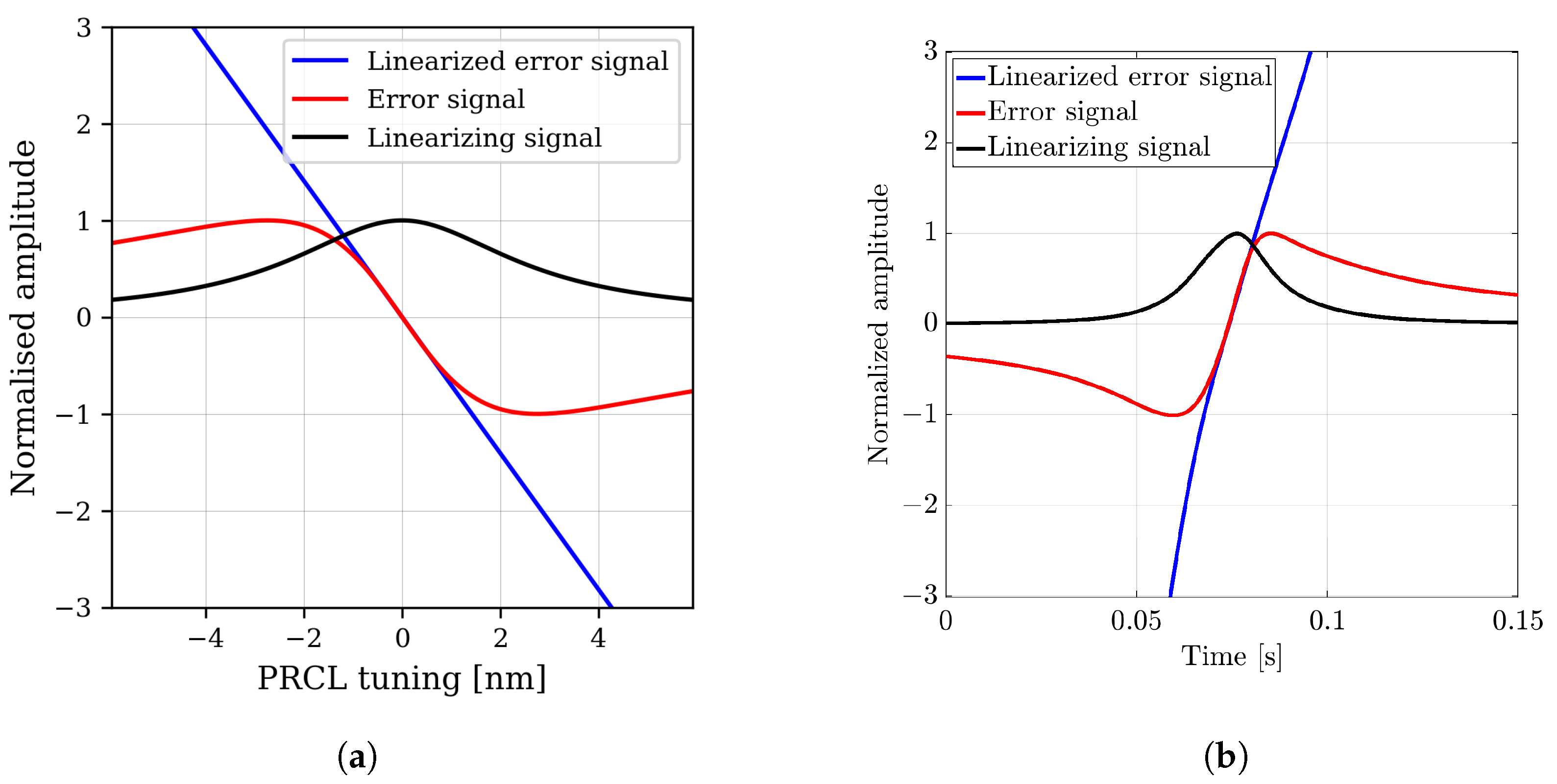
Linearization of the PRCL Error Signal
3. Trigger Logic for the Lock Acquisition
- The simulated DOFs are put in the foreseen working point in order to assess the behavior of the signals from the probes in the working point and its vicinity. This defines the expected values of the several signals (Figure 5);
- The aim is then to use only the information coming from the different probes to reconstruct as accurately as possible the working point. Given the relatively high number of DOFs, one single rule will not be enough for the determination of the working point; instead, adding one rule after the other, an inverse selection rules system is designed, constraining the working point of the several DOFs more and more as additional signals are used;
- The goodness of the trigger will depend on whether it ensures the correct selection of the wanted working point without leading to false positives.
- B4_12MHz_mag: beating of the 6 MHz upper and lower sidebands, probed in the Power-Recycling cavity; high values are expected when the three DOFs are on the working point since it is a measurement of the 6 MHz power (a value has been chosen);
- B1p_DC: DC of the dark port pick-off after the Signal-Recycling cavity; low values are expected when the three DOFs are on the working point (a value has been chosen);
- B4_112MHz_mag: beating of the 56 MHz upper and lower sidebands, probed in the Power-Recycling cavity; high values are expected when the three DOFs are on the working point since it is a measurement of the 56 MHz power (a value has been chosen);
- B4_DC: DC of the pick-off probed in the Power-Recycling cavity; low values are expected when the three DOFs are on the working point, as we want to lock on the sidebands and not on the Carrier (a value has been chosen).
4. Effects of Misalignments on the Longitudinal Error Signals
4.1. Methodology
- Base simulation of misaligned interferometer and convergence check;
- Simulation of the longitudinal DOF sweeps;
- Optimization and study of the error signals.
4.2. Simulation of Longitudinal Detunings
- Optical gains;
- Working point;
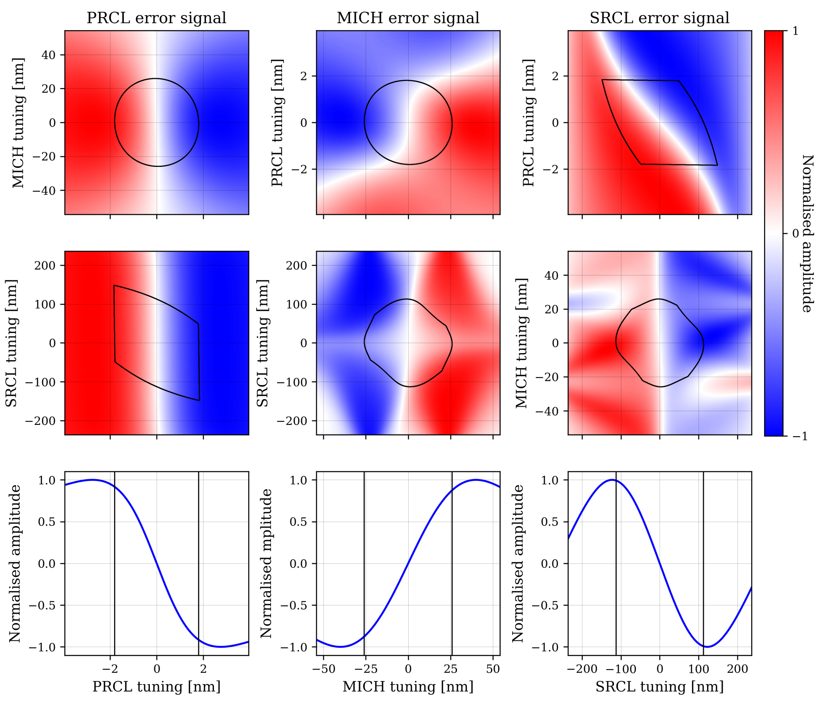
- Shape of the error signal (multiple zero crossings, etc.).
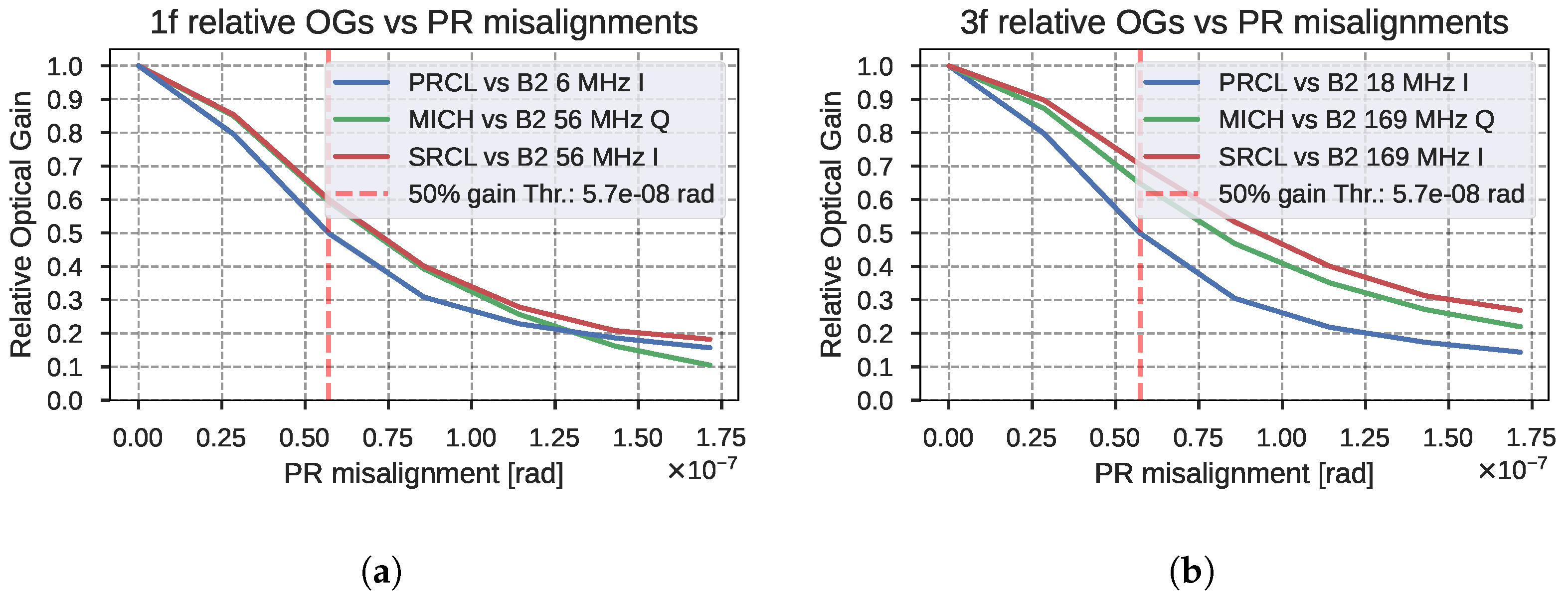
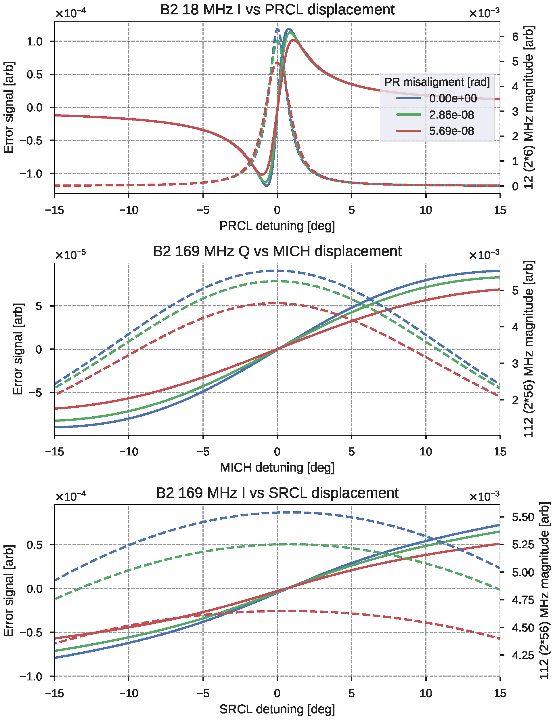
4.2.1. Optical Gain and Optimal Demodulation Phase Variations
4.2.2. Cross Couplings
4.2.3. Error Signal Shapes and Zero-Crossing
4.2.4. Results
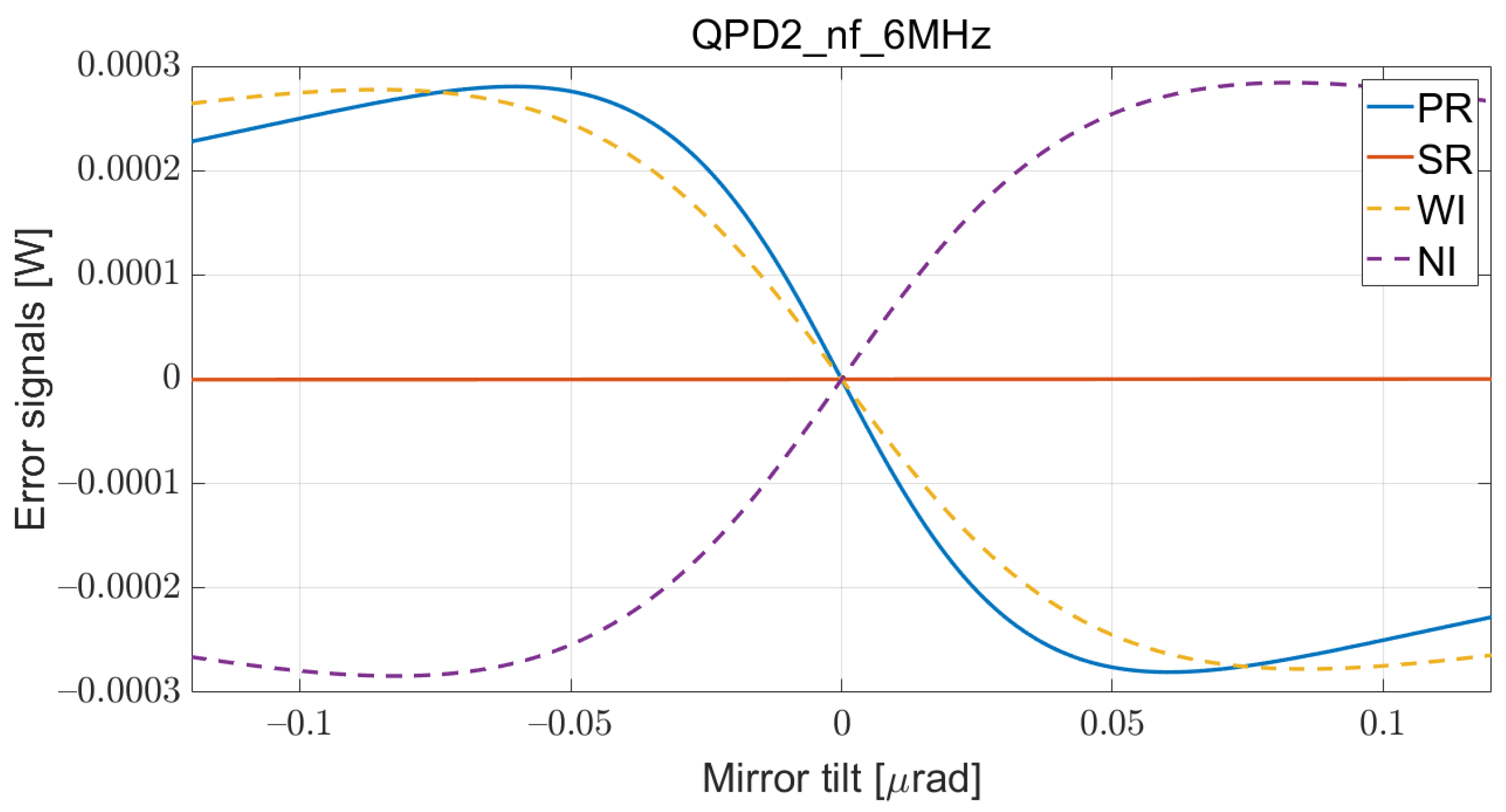
5. Alignment Controls
Simulation Results
6. Conclusions
- The error signals used to lock the longitudinal loops for both the initial acquisition and the intermediate state during the CARM offset reduction;
- The trigger signals used to determine the good conditions for the engagement of the feedback loops;
- The robustness of the chosen longitudinal error signals and the necessity of a global angular control of the PR mirror in order to maintain the lock during the whole lock acquisition procedure;
- The error signal for the aforementioned angular control of the PR mirror.
Author Contributions
Funding
Data Availability Statement
Acknowledgments
Conflicts of Interest
Abbreviations
| AdV+ | Advanced Virgo Plus |
| BNS | Binary Neutron Star |
| BS | Beam-Splitter |
| CARM | Common ARM |
| DOF | Degree Of Freedom |
| DRFPMI | Dual-Recycled Fabry-Pérot Michelson Interferometer |
| DRMI | Dual-Recycled Michelson Interferometer |
| EOM | Electro-Optic Modulator |
| HOM | Higher-Order Mode |
| INFN | Istituto Nazionale di Fisica Nucleare |
| IR | InfraRed |
| ITF | InTerFerometer |
| LIGO | Laser Interferometer Gravitational-Wave Observatory |
| LSC | Longitudinal Sensing and Control |
| MICH | short MICHelson length |
| NE | North-End |
| NF | Near-Field |
| NI | North Input |
| OG | Optical Gain |
| PDH | Pound-Drever-Hall |
| PR | Power-Recycling |
| PRC | Power-Recycling Cavity |
| PRCL | Power-Recycling Cavity Length |
| PRMI | Power-Recycled Michelson Interferometer |
| QPD | Quadrant PhotoDiode |
| SNR | Signal-to-Noise Ratio |
| SR | Signal Recycling |
| SRC | Signal-Recycling Cavity |
| SRCL | Signal-Recycling Cavity Length |
| TEM | Transverse Electro-Magnetic |
| UGF | Unity Gain Frequency |
| WE | West-End |
| WI | West Input |
Appendix A. Parameters of the Simulations

| Mirror | [m] | T | L |
|---|---|---|---|
| PR | 1430 | ||
| SR | 1430 | ||
| WI | |||
| NI |
- W
- m
- m
| [Hz] | Depth |
|---|---|
| 6,270,777 | |
| 8,361,036 | |
| 56,436,993 |
References
- Abbott, B.P.; Abbott, R.; Abbott, T.D.; Abraham, S.; Acernese, F.; Ackley, K.; Adams, C.; Adya, V.B.; Affeldt, C.; Agathos, M.; et al. Prospects for Observing and Localizing Gravitational-Wave Transients with Advanced LIGO, Advanced Virgo and KAGRA. Living Rev. Relativ. 2020, 23, 3. [Google Scholar] [CrossRef] [PubMed]
- Losurdo, G. Inertial Control of the VIRGO Superattenuator. AIP Conf. Proc. 2000, 523, 332–337. [Google Scholar] [CrossRef] [Green Version]
- Staley, A.; Martynov, D.; Abbott, R.; Adhikari, R.X.; Arai, K.; Ballmer, S.; Barsotti, L.; Brooks, A.F.; DeRosa, R.T.; Dwyer, S.; et al. Achieving Resonance in the Advanced LIGO Gravitational-Wave Interferometer. Class. Quantum Gravity 2014, 31, 245010. [Google Scholar] [CrossRef] [Green Version]
- De Rossi, C.; Brooks, J.; Casanueva Diaz, J.; Chiummo, A.; Genin, E.; Gosselin, M.; Leroy, N.; Mantovani, M.; Montanari, B.; Nocera, F.; et al. Development of a Frequency Tunable Green Laser Source for Advanced Virgo+ Gravitational Waves Detector. Galaxies 2020, 8, 87. [Google Scholar] [CrossRef]
- Acernese, F.; Amico, P.; Al-Shourbagy, M.; Aoudia, S.; Avino, S.; Babusci, D.; Ballardin, G.; Barillé, R.; Barone, F.; Barsotti, L.; et al. The Variable Finesse Locking Technique. Class. Quantum Gravity 2006, 23, S85–S89. [Google Scholar] [CrossRef]
- Drever, R.W.P.; Hall, J.L.; Kowalski, F.V.; Hough, J.; Ford, G.M.; Munley, A.J.; Ward, H. Laser Phase and Frequency Stabilization Using an Optical Resonator. Appl. Phys. B 1983, 31, 97–105. [Google Scholar] [CrossRef]
- Morrison, E.; Meers, B.J.; Robertson, D.I.; Ward, H. Automatic Alignment of Optical Interferometers. Appl. Opt. 1994, 33, 5041. [Google Scholar] [CrossRef] [PubMed]
- Brown, D.D.; Freise, A. Finesse. 2014. Available online: https://zenodo.org/record/821364#.Y5LNWn1BxPY (accessed on 20 January 2019). [CrossRef]
- Brown, D.D.; Jones, P.; Rowlinson, S.; Leavey, S.; Green, A.C.; Töyrä, D.; Freise, A. Pykat: Python Package for Modelling Precision Optical Interferometers. SoftwareX 2020, 12, 100613. [Google Scholar] [CrossRef]
- Yamamoto, H.; Barton, M.; Bhawal, B.; Evans, M.; Yoshida, S. Simulation Tools for Future Interferometers. In Journal of Physics: Conference Series; Mio, N., Ed.; IOPscience: Bristol, UK, 2006; Volume 32, pp. 398–403. [Google Scholar] [CrossRef]
- Casanueva Diaz, J.; Leroy, N. Auxiliary Laser System: Study of the Lock Acquisition Strategy; Technical Report VIR-0327B-19; Virgo Collaboration: Pisa, Italy, 2022; Available online: https://tds.virgo-gw.eu/ql/?c=14154 (accessed on 10 October 2022).
- Evans, M. Lock Acquisition in Resonant Optical Interferometers. Ph.D. Thesis, California Institute of Technology, Pasadena, CA, USA, 2002. Available online: https://labcit.ligo.caltech.edu/~mevans/lockAcq/thesis.pdf (accessed on 20 October 2022).
- Brown, D.; Rowlinson, S.; Leavey, S.; Jones, P.; Freise, A. Finesse 3. 2020. Available online: https://git.ligo.org/finesse/finesse3 (accessed on 20 October 2022).
- Allocca, A.; Bersanetti, D.; Casanueva Diaz, J.; De Rossi, C.; Mantovani, M.; Masserot, A.; Rolland, L.; Ruggi, P.; Swinkels, B.; Tapia San Martin, E.N.; et al. Interferometer Sensing and Control for the Advanced Virgo Experiment in the O3 Scientific Run. Galaxies 2020, 8, 85. [Google Scholar] [CrossRef]
- Allocca, A.; Chiummo, A.; Mantovani, M. Locking Strategy for the Advanced Virgo Central Interferometer; Technical Report VIR-0187A-16; Virgo Collaboration: Pisa, Italy, 2016; Available online: https://tds.virgo-gw.eu/ql/?c=11495 (accessed on 20 October 2022).
- Valentini, M.; Mantovani, M.; Casanueva Diaz, J.; Allocca, A.; Perreca, A. Effects of CITF Misalignments on the Longitudinal Error Signals during the CARM Offset Phase of AdV+; Technical Report VIR-0446B-20; Virgo Collaboration: Pisa, Italy, 2020; Available online: https://tds.virgo-gw.eu/ql/?c=15571 (accessed on 20 October 2022).
- Mason, J.E.; Willems, P.A. Signal Extraction and Optical Design for an Advanced Gravitational-Wave Interferometer. Appl. Opt. 2003, 42, 1269–1282. [Google Scholar] [CrossRef] [PubMed] [Green Version]
- Boldrini, M.; Casanueva Diaz, J.; Mantovani, M.; Majorana, E. Simulation of the Angular Sensing for the Central Interferometer in Advanced Virgo+; Technical Report VIR-0349C-21; Virgo Collaboration: Pisa, Italy, 2021; Available online: https://tds.virgo-gw.eu/ql/?c=16597 (accessed on 20 October 2022).
- Acernese, F.; Amico, P.; Arnaud, N.; Babusci, D.; Barillé, R.; Barone, F.; Barsotti, L.; Barsuglia, M.; Beauville, F.; Bizouard, M.A.; et al. A Local Control System for the Test Masses of the Virgo Gravitational Wave Detector. Astropart. Phys. 2004, 20, 617–628. [Google Scholar] [CrossRef]


| Lock Acquisition Step | PRCL | MICH | SRCL |
|---|---|---|---|
| Initial lock (“1f”) | B2 6 MHz | B2 56 MHz I | B2 56 MHz Q |
| CARM offset reduction (“3f”) | B2 18 MHz | B2 169 MHz I | B2 169 MHz Q |
| DOF | Signal | PR Thr. [Rad] | NI Thr. [Rad] | SR Thr. [Rad] |
|---|---|---|---|---|
| PRCL | B2 6 MHz I | N.A. | ||
| B2 18 MHz I | N.A. | |||
| MICH | B2 56 MHz I | N.A. | ||
| B2 169 MHz I | N.A. | |||
| SRCL | B2 56 MHz Q | N.A. | ||
| B2 169 MHz Q |
| DOF | Mag | Phase |
|---|---|---|
| PR | 72.80 dB | 89.10 |
| SR | 0.00 dB | −78.30 |
| NI | 70.02 dB | 89.10 |
| WI | 70.05 dB | 89.10 |
Publisher’s Note: MDPI stays neutral with regard to jurisdictional claims in published maps and institutional affiliations. |
© 2022 by the authors. Licensee MDPI, Basel, Switzerland. This article is an open access article distributed under the terms and conditions of the Creative Commons Attribution (CC BY) license (https://creativecommons.org/licenses/by/4.0/).
Share and Cite
Bersanetti, D.; Boldrini, M.; Diaz, J.C.; Freise, A.; Maggiore, R.; Mantovani, M.; Valentini, M. Simulations for the Locking and Alignment Strategy of the DRMI Configuration of the Advanced Virgo Plus Detector. Galaxies 2022, 10, 115. https://doi.org/10.3390/galaxies10060115
Bersanetti D, Boldrini M, Diaz JC, Freise A, Maggiore R, Mantovani M, Valentini M. Simulations for the Locking and Alignment Strategy of the DRMI Configuration of the Advanced Virgo Plus Detector. Galaxies. 2022; 10(6):115. https://doi.org/10.3390/galaxies10060115
Chicago/Turabian StyleBersanetti, Diego, Mattia Boldrini, Julia Casanueva Diaz, Andreas Freise, Riccardo Maggiore, Maddalena Mantovani, and Michele Valentini. 2022. "Simulations for the Locking and Alignment Strategy of the DRMI Configuration of the Advanced Virgo Plus Detector" Galaxies 10, no. 6: 115. https://doi.org/10.3390/galaxies10060115
APA StyleBersanetti, D., Boldrini, M., Diaz, J. C., Freise, A., Maggiore, R., Mantovani, M., & Valentini, M. (2022). Simulations for the Locking and Alignment Strategy of the DRMI Configuration of the Advanced Virgo Plus Detector. Galaxies, 10(6), 115. https://doi.org/10.3390/galaxies10060115