Abstract
We run a numerical experiment ejecting stellar winds in a very massive binary system measuring the properties of the resulting colliding wind structure and accreted mass onto the companion under different conditions. Colliding massive binaries interact and create a colliding wind structure with a shape that depends on the momentum ratio, orbital motion, distance between the stars, and other factors. We run simulations of a static LBV-WR binary and in each simulation abruptly varying the mass loss rate of the LBV from the fiducial value. The modified wind front propagates and interacts with the previous colliding wind structure, and modifies its shape. We calculate the emitted X-ray from the interaction and investigate the proprieties of the new shape. We derive the mass accretion rate onto the secondary, and find that it depends on the momentum ratio of the winds. We then add orbital velocity that reduces the mass accretion rate, a similar behaviour as the analytical estimates based on modified Bondi–Hoyle–Lyttleton. Creating a large set of simulations like those presented here can allow constraining parameters for specific colliding wind binaries and derive their stellar parameters and orbital solution.
1. Introduction
Very massive stars are known to blow strong winds that intensify as these stars evolve off the main-sequence (MS) (e.g., [1,2]). When a binary system has two stars that both eject winds, the two winds collide in a process which may produce observational signatures across the spectrum. Colliding wind systems appear in O and B stars and WR binaries, O-O stars, and LBV binaries [3,4,5,6,7]. They are also present in symbiotic systems, where ejecta from the WD collides with the AGB wind and produces soft X-ray emission (e.g., [8,9,10]), and in low-mass binaries (e.g., [11]).
Some colliding wind binaries present challenges to theory and common modelling, such as the Wolf–Rayet (WR) binary (or perhaps multiple) system Apep [12] that showed discrepancies in the observed wind velocities that suggest strongly anisotropic wind, never previously observed in colliding wind systems and challenging the understanding of WR winds. Presently colliding wind binary systems are being observed in the Magellanic clouds and in neighbouring galaxies (e.g., [13,14,15]). We will surely see more observations of such systems in the near future, and the field is ready for advanced theoretical interpretation with the aid of 3D hydrodynamic simulations.
The colliding wind structure (CWS) is classically defined as an infinitely long and thin axis-symmetric conical-like shape with thickness that varies with distance from the stars [5,6]. In the absence of orbital motion, its symmetry line is a line connecting the two stars. This structure is split by a contact discontinuity with two shock waves on both its sides. The shocked gas flows away along the sides of this conical-like structure. The shocked gas mainly resides between each of the two shocks and the contact discontinuity. The main parameter that determines the shape of the contact discontinuity is the momentum ratio of the two winds:
where and are the mass loss rate and the velocity of the wind of the secondary, and and are the same for the primary. The primary is considered to be the star with stronger wind, i.e., larger . Thus, in WR-O binary systems the WR is the primary, and in LBV-WR systems the LBV is the primary. From Equation (1), essentially , and in some cases (that will be studied in this paper) .
The ability of the shocked gas to dissipate its thermal energy affects the shape of the CWS. Radiative shocks manage to radiate away the thermal energy of the compressed gas and therefore cool and become thin and dense. It is also more prone to instabilities, such as the Rayleigh–Taylor instability and the non-linear thin shell instability (NTSI, [16,17]). If energy cannot be lost to radiation its only way to cool is by adiabatic expansion, thus the CWS with such adiabatic shocks is wider and has higher temperatures.
The asymptotic semi-opening angle of the CWS is obtained from a non-linear differential equation with being the only free parameter. It was calculated numerically by [18], and for intermediate values of there is an approximation derived by [19]:
which the authors state to be accurate to about 1%. It can be approximated, as done by [20] who approximated the contact discontinuity between the shocks as an hyperboloid, and gave analytic expressions for the width of the shocks (the distance from the contact discontinuity to the shock wave), on both sides. The expression for the shape of the CWS was later revisited a number of times (e.g., [21,22]).
Indeed, the actual shape of the CWS is more complicated, taking other factors into account. A partial list of these factors includes:
- The value of is location dependent, due to the acceleration of the wind.
- Clumps in the winds (small-scale inhomogeneities common in winds of massive stars; (e.g., [23,24,25]) make the CWS inhomogeneous.
- Instabilities arise when the winds collide, as a result of cooling that will form clumps in the colliding wind region.
- The radiation field of the secondary (the star with the weaker wind) may decelerate the primary incoming wind (radiative inhibition; [26,27]).
- Mixing can result in a range of flow speeds instead of a single uniform one [21].
- Orbital motion completely alters the CWS shape, making it rotate and wind around itself. In eccentric orbits the distance between the stars and the orbital velocity is time dependent, causing periodic modulation in the CWS.
Simulations of colliding wind binaries usually focused on one system with its particular conditions. To date, there is no set of general simulations that ran over a range of each of the parameters and isolated the influence of each physical effect. While covering a large parameter space is challenging and requires vast computational resources, isolating specific effects while restricting to a fiducial set of parameters is possible.
When the two winds are uneven in their momentum, accretion of primary gas to the secondary can take place. Accretion onto a companion star is a process that is only beginning to be studied in numerical simulations. Akashi et al. [28] were the first to derive accretion in a colliding wind binary simulation in which the secondary has a strong wind. They found that for the massive binary system Car mass is being accreted onto the companion close to periastron passage. A similar accretion process, though for a much longer period of time, was obtained for the O-O binary system HD 16674 [29].
Since the parameter space is very large it will have to be covered by large number of simulations. In this paper, as a first attempt, we run an experiment that quantifies accretion onto the secondary star, and the opening angle of the CWS.
2. Simulating Colliding Winds
We run the simulations using the hydrodynamic code FLASH, originally described by [30]. Our 3D Cartesian grid extends over , and . The grid is centred around the secondary star, and the orbital plane is on the plane. The grid has 5 levels of refinement. The largest cell has a side of ≃18 and the smallest has a side of ≃1.1 . The apex of the colliding winds has the second finest resolution, with resolution of ≃2.2 . To solve the hydrodynamic equations, we use the FLASH version of the dimensionally split piecewise parabolic method (PPM) solver [31]. The internal parts of the stars are not modelled and do not participate in the simulations. The gravity is treated as two-point gravity since self-gravity is not important. We include radiative cooling from [32]. The simulation includes radiation transfer with multigroup diffusion as implemented by the FLASH code. The simulations and post-processing described here were performed on the Ariel University GALAXY HPC cluster, for ∼ core-hours.
For most of the experiments presented here, the binary system remains stationary, and we do not include the orbital motion as the experiment aims to isolate the effects of the mass loss rate. We place the two stars at a distance of , and allow each star to accelerate their own wind. The mass loss rates of the primary and the secondary are and , respectively. The winds are ejected from a spherical layer above the star. The winds are radiatively accelerated according to the CAK model [33] force multiplier, with an acceleration that corresponds to for the primary and for the secondary. These values are motivated by a number of studies (e.g., [34,35]) and were chosen for simplicity. The acceleration also occurs outside the ejection zone. The terminal velocities are and . This gives a momentum ratio of . We name this set of parameters as Run 1, and treat it as our fiducial run. Figure 1 shows the density of the wind for the simulations we run. The stronger the primary wind, the smaller the opening angle of the colliding wind structure.
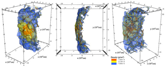
Figure 1.
The density of the wind for the simulations we run observed from 3 directions (our fiducial Run 1). The primary and the secondary are not shown. The side facing the secondary has finer clumps and filaments than the side facing the primary.
The winds blow for until the colliding wind structure extends to the edges of the grid, and then the experiment continues to the next step in which we turn to run the other simulations (runs listed below as 2–5). In Runs 2–5, we make a sudden transition of the mass loss rate of the primary, and by doing so lower the value of the momentum ratio . As it takes time for the wind to propagate, the change is not immediate, but rather takes time to establish. Table 1 lists the parameters of the simulations we run, as well as a summary of the results. Figure 2 shows density slices for some of our simulations.

Table 1.
Summary of simulations and results.
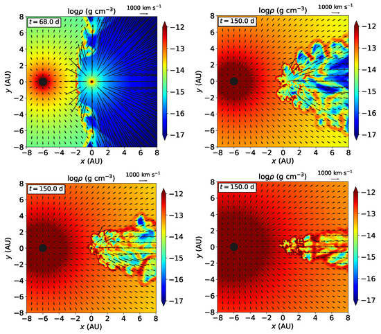
Figure 2.
The density of the wind for some of the simulations we run on a slice in the orbital plane. The primary is on the left side and the secondary is in the centre. Upper left: Run 1 (). Upper right: Run 2 (). Lower left: Run 3 (). Lower right: Run 5 ().
With the increase in the mass loss rate of the primary wind, the secondary wind and radiation cannot overcome the inflowing primary wind. Therefore, the secondary accretes mass from the primary wind. Let us describe the accretion process and the way we measure the accreted mass.
As the simulations run, the colliding wind experiences instabilities, especially in the side facing the secondary, that cools faster, and high-density clumps are formed. These clumps approach the injection zone of the secondary wind and even reach the cells of the secondary itself. A number of approaches are examined for the best numerical implementation for accretion [36], and we here briefly describe the one we use. To calculate the accreted mass we check whenever the actual density in a cell in the injection zone supersedes the expected undisturbed value of (expected as a result of the ejection of radiation-driven wind), and count the extra mass as accreted. Namely, the accreted mass is
where is the volume of the cell. The contributions from all cells in the injection zone are then summed up to obtain the total mass accreted for that time step. As the simulation time steps are much shorter than the duration of the accretion, this procedure brings accurate results. This process was tested in [29,36], where more details can be found. Figure 3 shows the mass accretion rate (lower panel) and the accreted mass as a function of time for Runs 2–5 (for Run 1 there is no accretion).
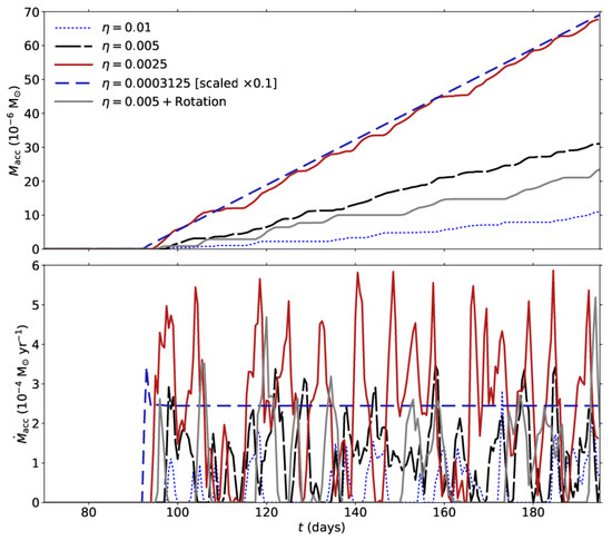
Figure 3.
(a) The total accreted mass. (b) The mass accretion rate. Note the different scaling for Run 6 (). The average accretion rate is given in Table 1 and Figure 7.
3. Results
Our runs continue for another 130 days, which is more than enough time for the new outflow to cover the entire grid and to obtain enough data for calculating average accretion rate, and X-ray luminosity, as we describe below. In one of the runs, Run 4, we include orbital motion in a circular orbit. This run can be compared with Run 3 that does not include orbital motion, as for both runs . A 3D density contour plot of this run is shown in Figure 4. The curving of the CWS is clearly seen. The orbital velocity in Run 4 is about a quarter of the wind velocity of the primary, namely, it has a moderate effect. The volume inside the cavity of the secondary wind does not include an undisturbed secondary wind but rather clumps from the colliding winds.
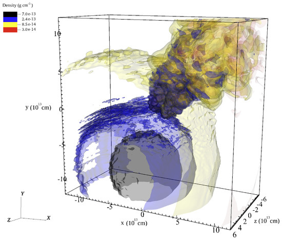
Figure 4.
A 3D density contour view of Run 4, that includes orbital motion at a time after reaching a quasi-steady state, namely, after the enhanced wind of the primary reached the whole simulation volume. The upper right corner shows the trailing of the colliding winds behind the secondary (located at the centre).
The X-ray emission is computed by interpolating from emission tables according to the implementation of the yt-project [37]. Figure 5 shows the 2–10 KeV X-ray emission on a slice of the simulation grid. For Run 1, the emission arrives from the colliding wind structure. For stronger mass loss rates in the rest of the runs, the emission arrives from shocks close to the secondary, and highlights the attempts of the secondary wind to blow against the collapsing clumps of the CWS around the secondary. As the figure shows, the smaller the value of , the more concentrated the emission on regions closer to the secondary.
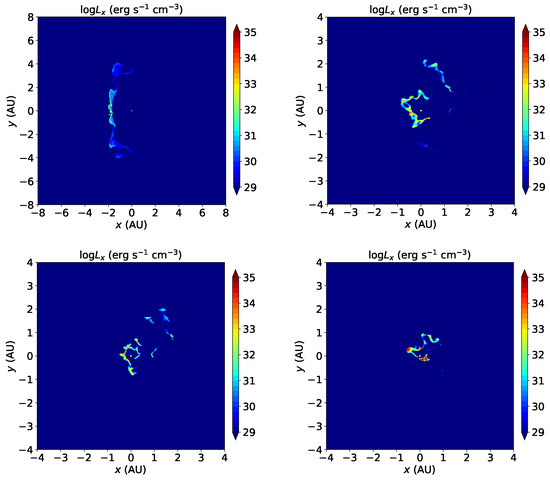
Figure 5.
The 2–10 KeV X-ray emission for the simulations we run on a slice in the orbital plane. The primary is on the left side and the secondary is in the centre. Upper left: Run 1. Upper right: Run 2. Lower left: Run 3. Lower right: Run 5. For Runs 2, 3, and 5, the emission is more concentrated and the plot is zoomed in on the emission region.
Figure 6 shows the X-ray luminosity emitted from the entire simulation grid, as a function of time. We do not include the absorption, which can be large and can greatly attenuate the observed flux by a large factor, and is also line-of-sight dependent. The enhancement in the mass loss rate of the primary creates a dense front that propagates and hits the colliding wind structure. As a result of this collision, the X-ray emission increases and a peak appears. After this time, which is the time that it takes for the intense wind to replace the quiescence wind (as in Run 1), the X-ray emission reaches a new quasi-stable level. The fluctuations in the level are the result of the interaction between the secondary wind that struggles to push against the primary wind.
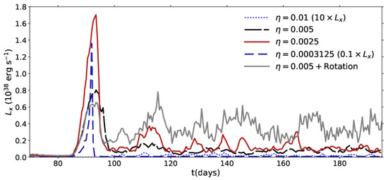
Figure 6.
The total emitted X-ray from the entire simulation grid (absorption is not included). Note the different scaling for some of the runs. The initial peak is the result of interaction of the enhanced wind with the previous CWS from the fiducial run (Run 1). The average X-ray luminosity (excluding the initial peak) is given in Table 1 and Figure 7. In Run 4 that included the orbital motion, the luminosity is stronger than in Run 3, which had the same parameters without orbital motion.
As explained above, we measure the mass accreted onto the secondary. In Run 1, no mass is accreted, but in all other runs, accretion onto the secondary takes place, either continuously or intermittently. Figure 7 shows the average mass accretion rate onto the secondary star (blue circles), and average X-ray emission luminosity (black squares). The grey symbols are for Run 4 that includes orbital motion. We find that the amount of mass accreted onto the secondary increases with decreasing , but not in a linear way. The accretion dependency on will be investigated in a future paper that will include more simulations. In this accretion domain, the X-ray emission is generally stronger for smaller , however, this trend breaks for Run 6 as the primary wind is so strong to the extent that the secondary wind almost cannot blow and therefore create shocks that emit X-rays.
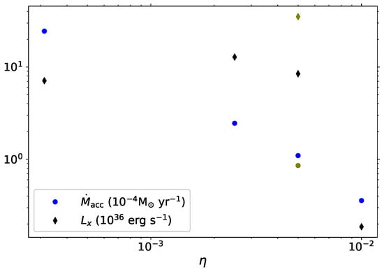
Figure 7.
Average mass accretion rate onto the secondary star (blue circles), and average X-ray emission luminosity (black squares). The average X-ray emission excludes the initial X-ray peak which is the result of interaction of the enhanced wind with the previous CWS from the fiducial run (Run 1). The orange symbols are for Run 4 that includes orbital motion.
Previous scaling relations of with have been proposed before based on theoretical arguments (e.g., [5]), and simulations (e.g., [22]). These were mostly obtained for adiabatic wind collisions. However, previous scaling relations are not applicable for very low as we examine here, especially when accretion takes place. Scaling relations as above use the total X-ray luminosity, which is a volume integrated quantity. They do not address the question of where the X-ray emission comes from, which is a different place than for higher values, as explained above and shown in Figure 5.
We use image processing methods to fit the shape line of the wind, an imaginary line dividing the turbulent flow into two domains, and the semi-opening angle, an asymptotic angle that describes the CWS. We use Canny edge detector [38], a multi-stage operation filter based on the derivative of a Gaussian, in order to compute the intensity of the gradients and by that determine a line that traces the shape of the wind. To reduce noise in the resulting image, we use morphological operations (dilation and erosion). Then, based on the shape of the wind and the location of the primary and secondary, we can derive the semi-opening angle of the wind. To obtain the optimal rays that form the opening angle, we calculate the Euclidean distance of each point in the line to the shape and sum over all the distances. We then minimise the function using the quasi-Newton BFGS method to obtain the best solution. Figure 8 shows the resulting opening angle for our six runs.
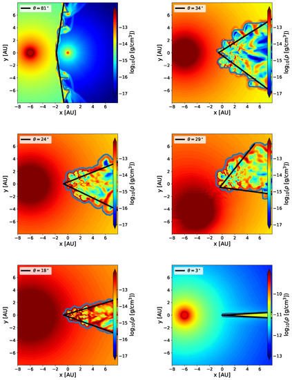
Figure 8.
A fit to the colliding wind structure semi-opening angle. The blue line is the result of the wind shape detection algorithm and the black line is the optimal line of an asymptotic opening. Upper left: Run 1. Upper right: Run 2. Middle left: Run 3. Middle right: Run 4. Lower left: Run 5. Lower right: Run 6 (note the different colour scale).
We plot the wind semi-opening angle as a function of in Figure 9. For most of our simulations, except Run 6, the simulations obtain larger opening angles than Equation (2). As we have an accelerating wind, is different at different locations, and this might affect the calculation. However, the more significant effect is the formation of instabilities, and requires the treatment we described above. For Run 6, we obtain a smaller semi-opening angle than the result from Equation (2). The equation is actually not applicable for such a small value of . In this run, the strong mass loss from the primary chokes the secondary wind almost completely. Therefore, the semi-opening angle does not really describe the same problem of colliding winds of two stars, but rather the collision of the primary wind with itself after being focused by the secondary and its gravitational field.
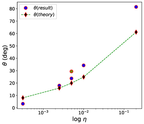
Figure 9.
Wind semi-opening angle at time . We include the theoretical value according to Equation (2) (marked ‘theory’; black squares) and the simulations results (blue circles).
4. Summary and Discussion
We explore the possibility of studying physical effects in colliding winds by simulating them in a systematic way. We start by quantifying a parameter that is not often discussed—accretion onto the companion star. We find that the mass accretion rate depends on the momentum ratio of the winds, and generally increases with decreasing . The instabilities have the velocity component in the direction of the flow but also have the acceleration of the secondary. Depending on the parameters, some of the clumps can be pulled towards the secondary and be accreted. In very low , the accretion is directly onto the secondary as there is no colliding wind structure. Our results also hint at saturation in the accreted mass for very low . The actual quantification of this dependency requires more simulations, which will be carried out in the near future.
We chose certain values for the mass loss rates and other parameters with the aim of describing a general system. These parameters do not represent the typical LBV-WR system. In future works, it will be necessary to check whether changing them makes a significant change in the results.
The accreted wind can have more effects, especially at high accretion rates. One of them is the reduction in the effective temperature of the secondary, as shown in [39]. At very high rates, the accreted gas might interact with the stellar envelope and modify the evolutionary path of the star. We do not model this in the present paper.
Our simulations also show that orbital motion reduces the mass accretion rate. This is in agreement with analytical estimates based on modified Bondi–Hoyle–Lyttleton. We note that the accretion is not Bondi–Hoyle–Lyttleton like and most of the accreted gas, it actually arrives from the side facing the primary and not from behind.
We also calculate the emitted 2–10 KeV X-ray luminosity from the colliding wind systems. The emission shows a first large peak at the time the enhanced wind of the primary reaches the pre-existing colliding wind structure. After that, there is a quiescence level of emission, associated with the new meta-stable colliding wind structure. The actual observed X-ray flux from such a system will depend on the absorption in the line of sight, and is expected to look different from different directions.
We used an advanced method to model the the colliding wind (asymptotic) semi-opening angle. While this practice is relevant for stationary stars, for orbiting stars it is not very well defined as the orbital motion curves the CWS, and the asymptotic semi-opening angle, are not well defined. We found that for most cases the angle is larger than the theoretical expression predicts, except for very small in which the assumptions of two winds that collide break and the primary wind in fact collides with itself.
The parameter space we chose here does not match particular systems. The aim of this work is to eventually be able to minimise the number of attempts required when performing simulations of real systems. For that, a better cover of the parameter space and especially testing simulations with different values of eccentricity is still needed. This present range of large mass accretion rates and very small values of can be helpful in simulating giant eruptions.
Running more simulations and modifying other parameters would allow a better understanding of the changes in the observables resulting from each of them. We expect such a process will be useful for studying specific massive binary wind systems, by reducing the number of attempts needed to simulate each system in order to match observations. This, in turn, will provide better constraints on massive colliding wind binaries’ physical properties.
Author Contributions
Conceptualisation, A.K. and A.M.; methodology, A.K. and A.M.; software, A.M.; formal analysis, A.K. and A.M.; writing—original draft preparation, A.K.; writing—review and editing, A.K. and A.M.; visualisation, A.K. and A.M. All authors have read and agreed to the published version of the manuscript.
Funding
This research received no external funding.
Acknowledgments
We thank the APN8 2021e organisers for a very interesting conference and for allowing us to present our work. We thank Noam Soker for very helpful discussions. We acknowledge the Ariel HPC Center at Ariel University for providing computing resources that have contributed to the research results reported within this paper.
Conflicts of Interest
The authors declare no conflict of interest.
References
- Langer, N. Presupernova Evolution of Massive Single and Binary Stars. Annu. Rev. Astron. Astrophys. 2012, 50, 107–164. [Google Scholar] [CrossRef]
- Vink, J.S. Very Massive Stars in the Local Universe. Proc. Int. Astron. Union 2012, 10, 51–79. [Google Scholar] [CrossRef]
- Parkin, E.R.; Pittard, J.M.; Hoare, M.G.; Wright, N.J.; Drake, J.J. 3D modelling of the colliding winds in η Carinae—Evidence for radiative inhibition. Mon. Not. R. Astron. Soc. 2009, 394, 1758–1774. [Google Scholar] [CrossRef]
- Parkin, E.R.; Pittard, J.M.; Corcoran, M.F.; Hamaguchi, K. Spiraling Out of Control: 3D Hydrodynamical Modeling of the Colliding Winds in η Carinae. Astrophys. J. 2011, 726, 105. [Google Scholar] [CrossRef]
- Stevens, I.R.; Blondin, J.M.; Pollock, A.M.T. Colliding Winds from Early-Type Stars in Binary Systems. Astrophys. J. 1992, 386, 265–287. [Google Scholar] [CrossRef]
- Usov, V.V. Stellar wind collision and X-ray generation in massive binaries. Astrophys. J. 1992, 389, 635–648. [Google Scholar] [CrossRef]
- Walder, R.; Folini, D. On the Stability of Colliding Flows: Radiative Shocks, Thin Shells, and Supersonic Turbulence. Astrophys. Space Sci. 2000, 274, 343–352. [Google Scholar] [CrossRef]
- Kenny, H.T.; Taylor, A.R. Colliding Winds in Symbiotic Binary Systems. I. Analytic and Numerical Solutions. Astrophys. J. 2005, 619, 527. [Google Scholar] [CrossRef]
- Kwok, S. Interacting stellar winds in a binary system. In Proceedings of the IAU Colloquium No. 59 Held in Miramare, Trieste, Italy, 15–19 September 1980. [Google Scholar]
- Sokoloski, J.L.; Lawrence, S.; Crotts, A.P.S.; Mukai, K. Flows and Shocks: Some Recent Developments in Symbiotic Star and Nova Research. arXiv 2017, arXiv:1702.05898. [Google Scholar]
- Johnstone, C.P.; Zhilkin, A.; Pilat-Lohinger, E.; Bisikalo, D.; Güdel, M.; Eggl, S. Colliding winds in low-mass binary star systems: Wind interactions and implications for habitable planets. Astron. Astrophys. 2015, 577, A122. [Google Scholar] [CrossRef][Green Version]
- Callingham, J.R.; Tuthill, P.G.; Pope, B.A.; Williams, P.M.; Crowther, P.A.; Edwards, M.; Norris, B.; Kedziora-Chudczer, L. Anisotropic winds in a Wolf-Rayet binary identify a potential gamma-ray burst progenitor. Nat. Astron. 2019, 3, 82–87. [Google Scholar] [CrossRef]
- Garofali, K.; Levesque, E.M.; Massey, P.; Williams, B.F. The First Candidate Colliding-wind Binary in M33. Astrophys. J. 2019, 880, 8. [Google Scholar] [CrossRef]
- Shenar, T.; Sana, H.; Marchant, P.; Pablo, B.; Richardson, N.; Moffat, A.F.J.; Van Reeth, T.; Barbá, R.H.; Bowman, D.M.; Broos, P.; et al. The Tarantula Massive Binary Monitoring. V. R 144: A wind-eclipsing binary with a total mass ≥ 140 M⊙. Astron. Astrophys. 2021, 650, A147. [Google Scholar] [CrossRef]
- Williams, P.M.; Morrell, N.I.; Boutsia, K.; Massey, P. The episodic dust-making Wolf-Rayet star HD 38030 in the Large Magellanic Cloud. Mon. Not. R. Astron. Soc. 2021, 505, 5029–5037. [Google Scholar] [CrossRef]
- Kee, N.D.; Owocki, S.; Ud-Doula, A. Suppression of X-rays from radiative shocks by their thin-shell instability. Mon. Not. R. Astron. Soc. 2014, 438, 3557–3567. [Google Scholar] [CrossRef]
- Vishniac, E.T. ApJ, 428, 186: Nonlinear instabilities in shock-bounded slabs. Astrophys. J. 1994, 428, 186–208. [Google Scholar] [CrossRef]
- Girard, T.; Willson, L.A. Winds in collision. III. Modeling the interaction nebulae of eruptive symbiotics. Astron. Astrophys. 1987, 183, 247–256. [Google Scholar]
- Eichler, D.; Usov, V. Particle acceleration and nonthermal radio emission in binaries of early-type stars. Astrophys. J. 1993, 402, 271–279. [Google Scholar] [CrossRef]
- Kashi, A.; Soker, N. Modelling the radio light curve of η Carinae. Mon. Not. R. Astron. Soc. 2007, 378, 1609–1618. [Google Scholar] [CrossRef]
- Gayley, K.G. Asymptotic Opening Angles for Colliding-Wind Bow Shocks: The Characteristic-Angle Approximation. Astrophys. J. 2009, 703, 89. [Google Scholar] [CrossRef]
- Pittard, J.M.; Dawson, B. Colliding stellar winds structure and X-ray emission. Mon. Not. R. Astron. Soc. 2018, 477, 5640–5645. [Google Scholar] [CrossRef]
- Crowther, P.A.; Dessart, L.; Hillier, D.J.; Abbott, J.B.; Fullerton, A.W. Stellar and wind properties of LMC WC4 stars. A metallicity dependence for Wolf-Rayet mass-loss rates. Astron. Astrophys. 2002, 392, 653–669. [Google Scholar] [CrossRef]
- Moffat, A.F.J. Clumping in Hot-Star Winds, 17: Observational Overview of Clumping in Hot Stellar Winds; Universität Potsdam: Potsdam, Germany, 2008. [Google Scholar]
- Walder, R.; Folini, D. Theoretical Considerations on Colliding Clumped Winds. arXiv 2002, arXiv:astro-ph/0012133. [Google Scholar]
- Gayley, K.G.; Owocki, S.P.; Cranmer, S.R. Sudden Radiative Braking in Colliding Hot-Star Winds. Astrophys. J. 1997, 475, 786. [Google Scholar] [CrossRef]
- Owocki, S.P.; Gayley, K.G. The Importance of Radiative Braking for the Wind Interaction in the Close WR+O Binary V444 Cygni. Astrophys. J. Lett. 1995, 454, L145. [Google Scholar] [CrossRef]
- Akashi, M.S.; Kashi, A.; Soker, N. Accretion of dense clumps in the periastron passage of η Carinae. New Astron. 2013, 18, 23–30. [Google Scholar] [CrossRef]
- Kashi, A. Wind collision and accretion simulations of the massive binary system HD 166734. Mon. Not. R. Astron. Soc. 2020, 492, 5261–5270. [Google Scholar] [CrossRef]
- Fryxell, B.; Olson, K.; Ricker, P.; Timmes, F.X.; Zingale, M.; Lamb, D.Q.; MacNeice, P.; Rosner, R.; Truran, J.W.; Tufo, H. FLASH: An Adaptive Mesh Hydrodynamics Code for Modeling Astrophysical Thermonuclear Flashes. Astrophys. J. Suppl. Ser. 2000, 131, 273. [Google Scholar] [CrossRef]
- Colella, P.; Woodward, P.R. The Piecewise Parabolic Method (PPM) for Gas-Dynamical Simulations. J. Comput. Phys. 1984, 54, 174–201. [Google Scholar] [CrossRef]
- Sutherland, R.S.; Dopita, M.A. Cooling functions for low-density astrophysical plasmas. Astrophys. J. Suppl. Ser. 1993, 88, 253. [Google Scholar] [CrossRef]
- Castor, J.I.; Abbott, D.C.; Klein, R.I. Radiation-driven winds in Of stars. Astrophys. J. 1975, 195, 157–174. [Google Scholar] [CrossRef]
- Müller, P.E.; Vink, J.S. A consistent solution for the velocity field and mass-loss rate of massive stars. Astron. Astrophys. 2008, 492, 493–509. [Google Scholar] [CrossRef]
- Pauldrach, A.; Puls, J.; Kudritzki, R.P. Radiation-driven winds of hot luminous stars. Improvements of the theory and first results. Astron. Astrophys. 1986, 164, 86–100. [Google Scholar]
- Kashi, A. Simulating the Response of the Secondary Star of Eta Carinae to Mass Accretion at Periastron Passage. Mon. Not. R. Astron. Soc. 2019, 486, 926–935. [Google Scholar] [CrossRef]
- Turk, M.J.; Smith, B.D.; Oishi, J.S.; Skory, S.; Skillman, S.W.; Abel, T.; Norman, M.L. Yt: A Multi-code Analysis Toolkit for Astrophysical Simulation Data. Astrophys. J. Suppl. Ser. 2011, 192, 9. [Google Scholar] [CrossRef]
- Canny, J. A Computational Approach to Edge Detection. IEEE Trans. Pattern Anal. Mach. Intell. 1986, PAMI-8, 679–698. [Google Scholar] [CrossRef]
- Kashi, A. Accretion at the periastron passage of Eta Carinae. Mon. Not. R. Astron. Soc. 2017, 464, 775–782. [Google Scholar] [CrossRef][Green Version]
Publisher’s Note: MDPI stays neutral with regard to jurisdictional claims in published maps and institutional affiliations. |
© 2021 by the authors. Licensee MDPI, Basel, Switzerland. This article is an open access article distributed under the terms and conditions of the Creative Commons Attribution (CC BY) license (https://creativecommons.org/licenses/by/4.0/).