
Flexible Risk Evidence Combination Rules in Breast Cancer Precision Therapy

 , ,
, ,  , and
, and
Abstract
1. Introduction
2. Materials and Methods
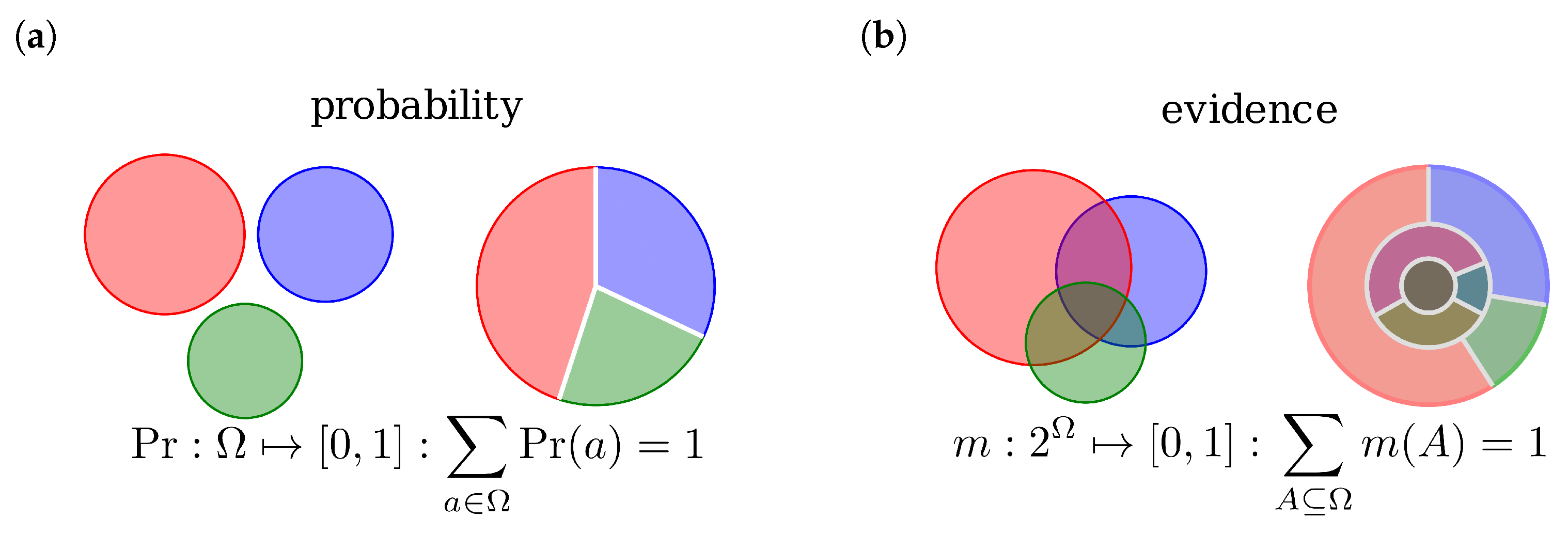
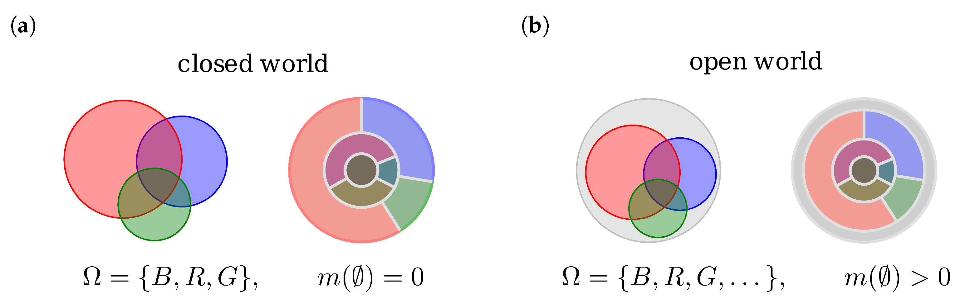
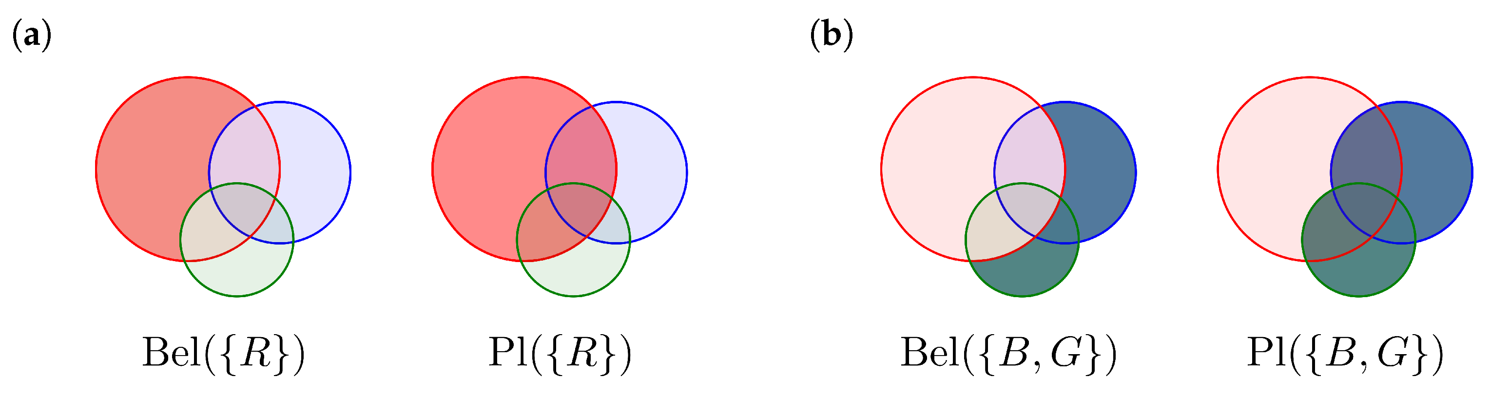
2.1. Dempster-Shafer Theory
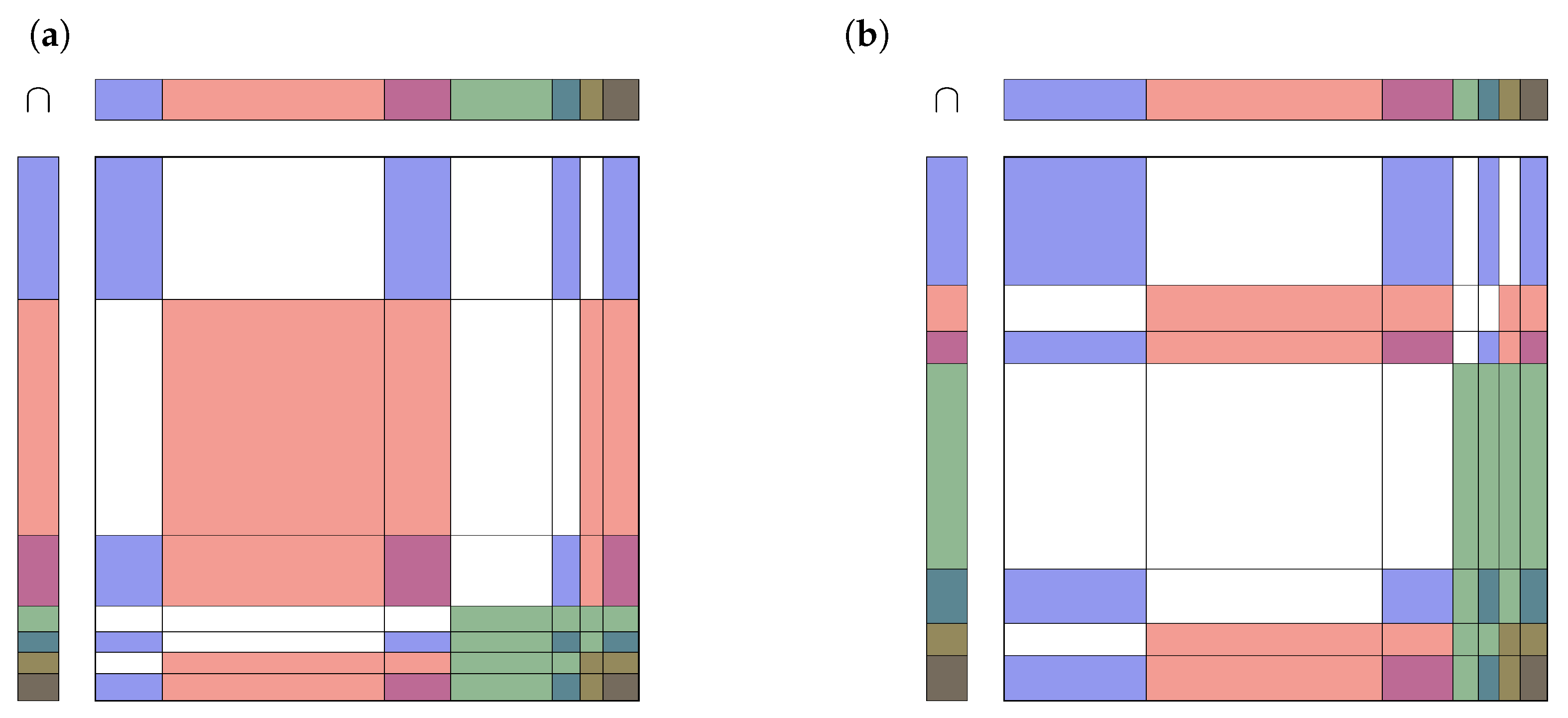
2.2. Evidence Combination Rules
3. Results
3.1. Model Adaptation
- The operator ⊗, as defined in Formula (8), is not fully compatible with DST. There is always a dependence between the two receptor status. However, DST in its original form requires independent BBMs. This is obviously not the case for estrogen and progesterone receptors. Our suggestion to absorb this correlation is to replace ⊗ by giving estrogen and progesterone a balanced contribution to both BBM.
- The operator for combining pieces of evidence coming from gene expression and co-gene expression might be problematic in case of conflicting expression values. In a previous paper [32] we introduced mass limits and for the BBMs to tackle this issue. We retain these mass limits, but replace by as an additional reinsurance.
- Combining gene expression evidence with IHC evidence, the operator will in case of conflict put too much weight into the mass of ignorance, . Therefore we suggest slightly increasing and replacing by . On the lower end of the -range, the influence of on the ECR is significantly less than on the upper end. As long as there is a profound confidence in the data, particularly in the IHC measurements, replacing by e.g., is therefore also an option.
- In the past it turned out that the optimal choice for the co-gene of progesterone is mostly estrogen itself. If so, although and are calculated differently and so vary numerically, they are basically generated from the same gene expression data. A preferable assumption in DST is the independence of input data to generate evidence. In contrary to estrogen, progesterone expression data is often diffuse and it might be impossible to find a decent co-gene. This issue can be easily resolved by replacing with the vacuous mass function. Currently, for the sake of consistency, we stick to the current configuration which uses estrogen as co-gene for progesterone.
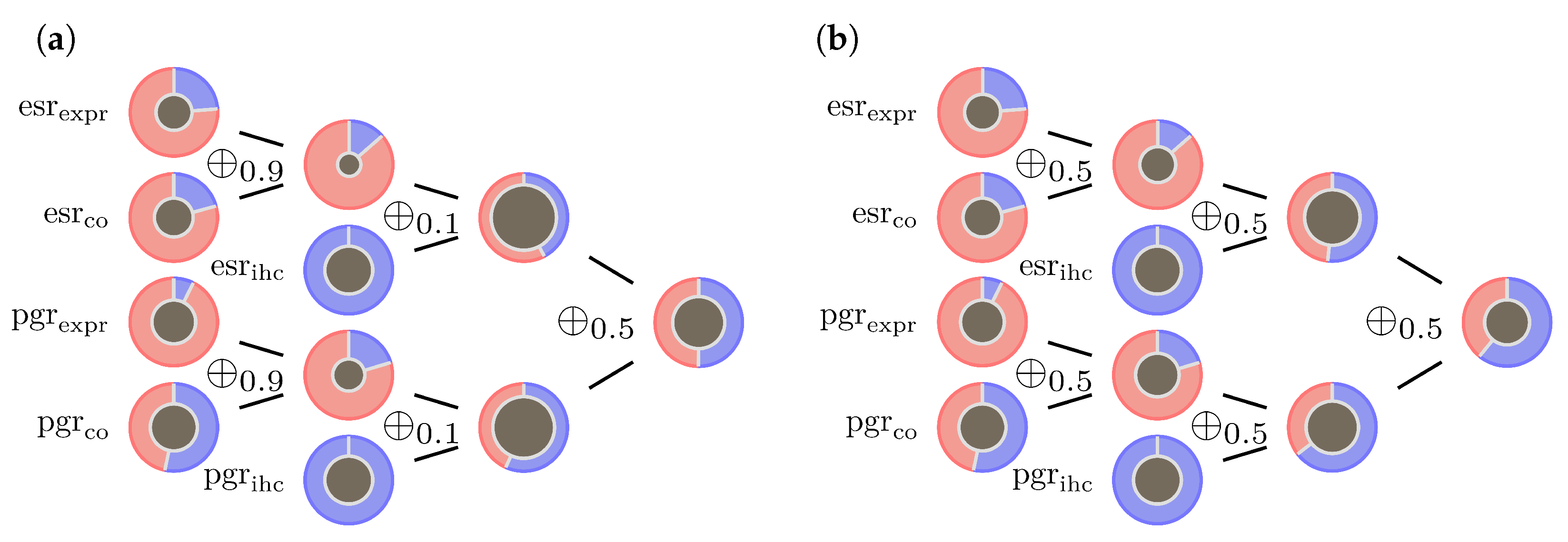
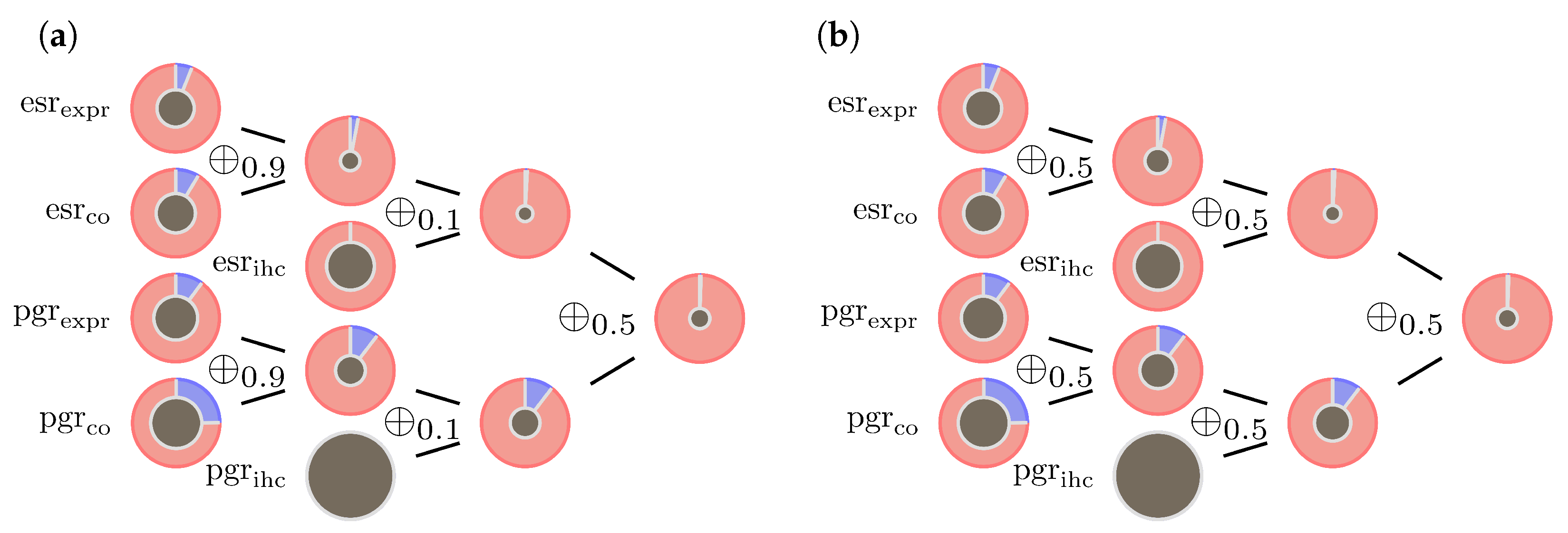
3.2. Examples
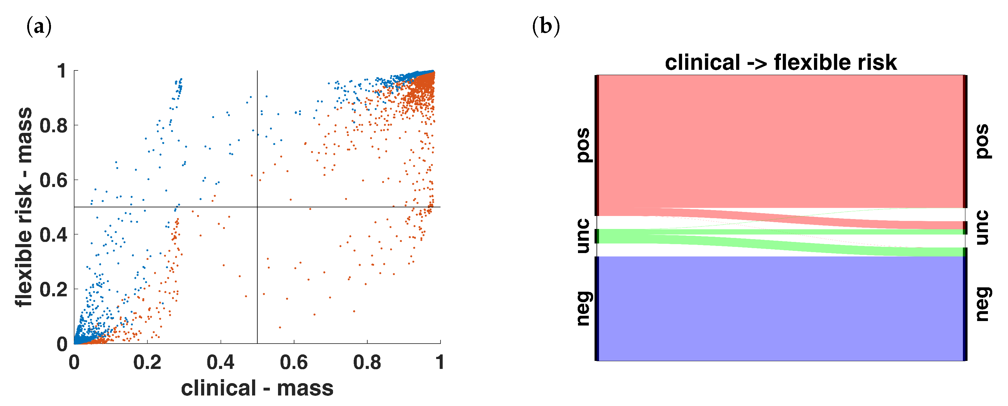
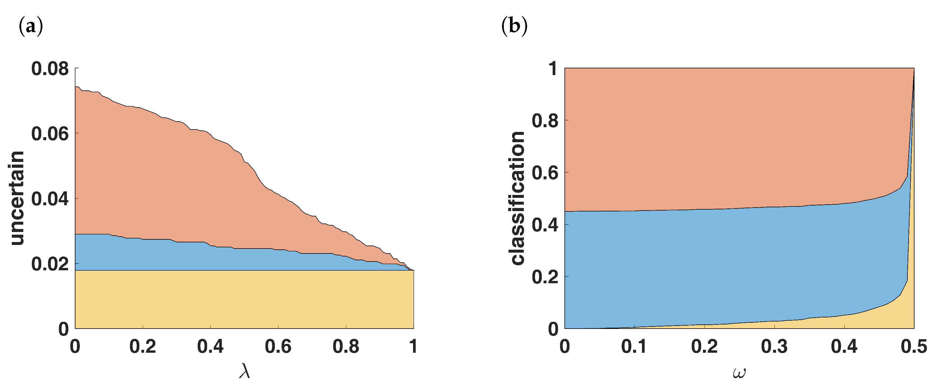
3.3. Analysis
3.4. Decision Making
4. Discussion
4.1. Quality of Data
4.2. From Data to Evidence
4.3. The Functionality of in
4.4. Training of in on Real Data
4.5. Enhanced Evidence Combination Rules
4.6. An Evidence Combination Rule with Constant Ignorance
4.7. Modified Frame of Discernment
4.8. Risk Function for Decision Making
5. Conclusions
Author Contributions
Funding
Institutional Review Board Statement
Informed Consent Statement
Data Availability Statement
Acknowledgments
Conflicts of Interest
Abbreviations
| BBM | basic belief masses, same as basic belief assignment (BBA) |
| BC | breast cancer |
| DSmT | Dezert-Smarandache theory |
| DST | Dempster-Shafer theory of evidence |
| ECR | evidence combination rule |
| ESR | estrogen |
| FOD | frame of discernment |
| GEO | Gene Expression Omnibus |
| IHC | immunohistochemistry |
| PCR | proportional conflict redistribution |
| PGR | progesterone |
| SLAM | simultaneous localization and mapping |
| TBM | transferable belief model |
Appendix A. Examples of Combining Pieces of Evidence
Appendix A.1. Two Rather Consistent Agents

Appendix A.2. Two Rather Contradictory Agents

Appendix B. Data Description
References
- Dempster, A. Upper and Lower Probabilities Induced by a Multivalued Mapping. Ann. Math. Stat. 1967, 38, 325–339. [Google Scholar] [CrossRef]
- Dempster, A.P. A Generalization of Bayesian Inference. J. R. Stat. Soc. Ser. B (Methodol.) 1968, 30, 205–232. [Google Scholar] [CrossRef]
- Vallverdú, J. Bayesians versus Frequentists a Philosophical Debate on Statistical Reasoning; Springer Briefs in Statistics; Springer: Berlin/Heidelberg, Germany, 2016; p. 110. [Google Scholar]
- Shafer, G. A Mathematical Theory of Evidence; Princeton University Press: Princeton, NJ, USA, 1976. [Google Scholar]
- Zadeh, L.A. A Simple View of the Dempster-Shafer Theory of Evidence and Its Implication for the Rule of Combination. AI Mag. 1986, 7, 85–90. [Google Scholar]
- Smets, P.; Mamdani, A.; Dubois, D.; Prade, H. Non-Standard Logics for Automated Reasoning; Academic Press: New York, NY, USA, 1988. [Google Scholar]
- Dubois, D.; Prade, H. Representation and combination of uncertainty with belief functions and possibility measures. Comput. Intell. 1988, 4, 244–264. [Google Scholar] [CrossRef]
- Smets, P. The Combination of Evidence in the Transferable Belief Model. IEEE Trans. Pattern Anal. Mach. Intell. 1990, 12, 447–458. [Google Scholar] [CrossRef]
- Denoeux, T. Analysis of evidence-theoretic decision rules for pattern classification. Pattern Recognit. 1997, 30, 1095–1107. [Google Scholar] [CrossRef]
- Smets, P. The Nature of the unnormalized Beliefs encountered in the Transferable Belief Model. In Uncertainty in Artificial Intelligence; Dubois, D., Wellman, M.P., D’Ambrosio, B., Smets, P., Eds.; Morgan Kaufmann: Burlington, MA, USA, 1992; pp. 292–297. [Google Scholar] [CrossRef]
- Smets, P. Belief functions: The disjunctive rule of combination and the generalized Bayesian theorem. Int. J. Approx. Reason. 1993, 9, 1–35. [Google Scholar] [CrossRef]
- Smets, P.; Kennes, R. The transferable belief model. Artif. Intell. 1994, 66, 191–234. [Google Scholar] [CrossRef]
- Kohlas, J.; Monney, P.A. A mathematical Theory of Hints: An Approach to the Dempster-Shafer Theory of Evidence, 1st ed.; Lecture Notes in Economics and Mathematical Systems; Springer: Berlin/Heidelberg, Germany, 1995. [Google Scholar]
- Gebhardt, J.; Kruse, R. The context model: An integrating view of vagueness and uncertainty. Int. J. Approx. Reason. 1993, 9, 283–314. [Google Scholar] [CrossRef]
- Smarandache, F.; Dezert, J. Proportional Conflict Redistribution Rules for Information Fusion. Adv. Appl. DSmT Inf. Fusion (Collect. Work.) 2006, 2, 3–68. [Google Scholar]
- Yager, R.R. On the dempster-shafer framework and new combination rules. Inf. Sci. 1987, 41, 93–137. [Google Scholar] [CrossRef]
- Sentz, K.; Ferson, S. Combination of Evidence in Dempster-Shafer Theory. In Sandia Report; Sand 2002-0835; Sandia National Laboratories: Albuquerque, NM, USA; Livermore, CA, USA, 2002. [Google Scholar]
- Yang, J.B.; Xu, D.L. Evidential reasoning rule for evidence combination. Artif. Intell. 2013, 205, 1–29. [Google Scholar] [CrossRef]
- Smarandache, F.; Dezert, J. Information fusion based on new proportional conflict redistribution rules. In Proceedings of the 2005 7th International Conference on Information Fusion, Philadelphia, PA, USA, 25–28 July 2005; Volume 2, p. 8. [Google Scholar] [CrossRef]
- Smarandache, F.; Dezert, J.; Tacnet, J. Fusion of sources of evidence with different importances and reliabilities. In Proceedings of the 2010 13th International Conference on Information Fusion, Edinburgh, UK, 26–29 July 2010; pp. 1–8. [Google Scholar] [CrossRef]
- Dezert, T.; Dezert, J. Improvement of Proportional Conflict Redistribution Fusion Rules for Levee Characterization. In Proceedings of the ESREL 2021, Angers, France, 19–23 September 2021. [Google Scholar]
- Smets, P. Constructing the Pignistic Probability Function in a Context of Uncertainty. In Machine Intelligence and Pattern Recognition; Henrion, M., Shachter, R.D., Kanal, L.N., Lemmer, J.F., Eds.; Elsevier: Amsterdam, The Netherlands, 1990; Volume 10, pp. 29–39. [Google Scholar] [CrossRef]
- Von Neumann, J.; Morgenstern, O. Theory of Games and Economic Behavior, 3rd ed.; Princeton University Press: Princeton, NJ, USA, 1953. [Google Scholar]
- Von Neumann, J.; Morgenstern, O.; Kuhn, H.; Rubinstein, A. Theory of Games and Economic Behavior: 60th Anniversary Commemorative Edition, 4th ed.; Princeton University Press: Princeton, NJ, USA, 2007. [Google Scholar]
- Denœux, T. Decision-making with belief functions: A review. Int. J. Approx. Reason. 2019, 109, 87–110. [Google Scholar] [CrossRef]
- Reineking, T. Belief Functions: Theory and Algorithms. Ph.D. Thesis, Universität Bremen, Bremen, Germany, 2014. [Google Scholar]
- Al-Ani, A.; Deriche, M. A new technique for combining multiple classifiers using the Dempster-Shafer theory of evidence. J. Artif. Intell. Res. 2002, 17, 333–361. [Google Scholar] [CrossRef]
- Mandler, E.; Schümann, J. Combining the Classification Results of Independent Classifiers Based on the Dempster/Shafer Theory of Evidence. Mach. Intell. Pattern Recognit. 1988, 7, 381–393. [Google Scholar] [CrossRef]
- Dezert, J.; Tchamova, A. On the Validity of Dempster’s Fusion Rule and its Interpretation as a Generalization of Bayesian Fusion Rule. Int. J. Intell. Syst. 2014, 29, 223–252. [Google Scholar] [CrossRef]
- Bourbaki, N. Algebra I: Chapters 1–3; Springer: Heidelberg, Germany, 1989. [Google Scholar]
- Inagaki, T. Interdependence between safety-control policy and multiple-sensor schemes via Dempster-Shafer theory. IEEE Trans. Reliab. 1991, 40, 182–188. [Google Scholar] [CrossRef]
- Kenn, M.; Cacsire Castillo-Tong, D.; Singer, C.F.; Karch, R.; Cibena, M.; Koelbl, H.; Schreiner, W. Decision theory for precision therapy of breast cancer. Sci. Rep. 2021, 11, 4233. [Google Scholar] [CrossRef] [PubMed]
- Kenn, M.; Karch, R.; Cacsire Castillo-Tong, D.; Singer, C.F.; Koelbl, H.; Schreiner, W. Decision Theory versus Conventional Statistics for Personalized Therapy of Breast Cancer. J. Pers. Med. 2022, 12, 570. [Google Scholar] [CrossRef] [PubMed]
- Edgar, R.; Domrachev, M.; Lash, A.E. Gene Expression Omnibus: NCBI gene expression and hybridization array data repository. Nucleic Acids Res. 2002, 30, 207–210. [Google Scholar] [CrossRef] [PubMed]


| (a) | ||||
| flexible risk | ||||
| pos | unc | neg | ||
| clinical | pos | 1287 | 78 | 1 |
| unc | 3 | 51 | 86 | |
| neg | 0 | 0 | 1013 | |
| (b) | ||||
| constant | ||||
| pos | unc | neg | ||
| flexible risk | pos | 1268 | 22 | 0 |
| unc | 14 | 107 | 8 | |
| neg | 0 | 2 | 1098 | |
Disclaimer/Publisher’s Note: The statements, opinions and data contained in all publications are solely those of the individual author(s) and contributor(s) and not of MDPI and/or the editor(s). MDPI and/or the editor(s) disclaim responsibility for any injury to people or property resulting from any ideas, methods, instructions or products referred to in the content. |
© 2023 by the authors. Licensee MDPI, Basel, Switzerland. This article is an open access article distributed under the terms and conditions of the Creative Commons Attribution (CC BY) license (https://creativecommons.org/licenses/by/4.0/).
Share and Cite
Kenn, M.; Karch, R.; Singer, C.F.; Dorffner, G.; Schreiner, W. Flexible Risk Evidence Combination Rules in Breast Cancer Precision Therapy. J. Pers. Med. 2023, 13, 119. https://doi.org/10.3390/jpm13010119
Kenn M, Karch R, Singer CF, Dorffner G, Schreiner W. Flexible Risk Evidence Combination Rules in Breast Cancer Precision Therapy. Journal of Personalized Medicine. 2023; 13(1):119. https://doi.org/10.3390/jpm13010119
Chicago/Turabian StyleKenn, Michael, Rudolf Karch, Christian F. Singer, Georg Dorffner, and Wolfgang Schreiner. 2023. "Flexible Risk Evidence Combination Rules in Breast Cancer Precision Therapy" Journal of Personalized Medicine 13, no. 1: 119. https://doi.org/10.3390/jpm13010119
APA StyleKenn, M., Karch, R., Singer, C. F., Dorffner, G., & Schreiner, W. (2023). Flexible Risk Evidence Combination Rules in Breast Cancer Precision Therapy. Journal of Personalized Medicine, 13(1), 119. https://doi.org/10.3390/jpm13010119