The Impact of Weighting Factors on Dual-Energy Computed Tomography Image Quality in Non-Contrast Head Examinations: Phantom and Patient Study

 , , , ,
  and
and
Abstract
1. Introduction
2. Materials and Methods
2.1. Phantom Study
2.1.1. CT Protocol and Image Processing
2.1.2. Quantitative Image Analysis
2.1.3. Qualitative Image Analysis
- No or minimal noise or artifacts, excellent GM/WM contrast and overall IQ.
- Some noise and artifacts that do not influence image evaluation, very good GM/WM contrast and overall IQ.
- Noise and artifacts that allow limited evaluation, poor GM/WM contrast and overall IQ.
- Too much noise-uninterpretable, no GM/WM contrast, non-diagnostic images.
2.1.4. Impact of Dose Variations on Image Quality
2.2. Patient Study
Quantitative and Qualitative Image Quality Analysis
2.3. Statistical Analysis
3. Results
3.1. Phantom Study
Impact of Dose Variations on Image Quality
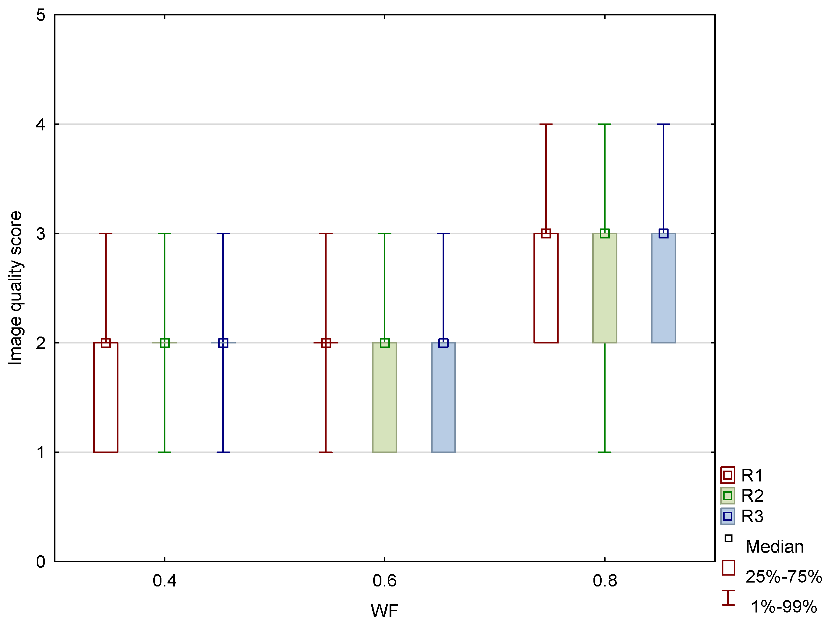
3.2. Patient Study
4. Discussion
5. Conclusions
Author Contributions
Funding
Institutional Review Board Statement
Informed Consent Statement
Data Availability Statement
Conflicts of Interest
References
- Goo, H.W.; Goo, J.M. Dual-Energy CT: New Horizon in Medical Imaging. Korean Radiol. Soc. 2017, 18, 555–569. [Google Scholar] [CrossRef] [PubMed]
- Hamid, S.; Nasir, M.U.; So, A.; Andrews, G.; Nicolaou, S.; Qamar, S.R. Clinical Applications of Dual-Energy CT. Korean Radiol. Soc. 2021, 22, 970–982. [Google Scholar] [CrossRef] [PubMed]
- Odedra, D.; Narayanasamy, S.; Sabongui, S.; Priya, S.; Krishna, S.; Sheikh, A. Dual Energy CT Physics—A Primer for the Emergency Radiologist. Front. Radiol. 2022, 2, 820430. [Google Scholar] [CrossRef] [PubMed]
- Borges, A.P.; Antunes, C.; Curvo-Semedo, L. Pros and Cons of Dual-Energy CT Systems: “One Does Not Fit All”. Tomography 2023, 9, 195–216. [Google Scholar] [CrossRef]
- Kucinski, T. Unenhanced CT and Acute Stroke Physiology. Neuroimaging Clin. N. Am. 2005, 15, 397–407. [Google Scholar] [CrossRef]
- Postma, A.A.; Das, M.; Stadler, A.A.R.; Wildberger, J.E. Dual-Energy CT: What the Neuroradiologist Should Know. Curr. Radiol. Rep. 2015, 3, 16. [Google Scholar] [CrossRef]
- Gibney, B.; Redmond, C.E.; Byrne, D.; Mathur, S.; Murray, N. A Review of the Applications of Dual-Energy CT in Acute Neuroimaging. Can. Assoc. Radiol. J. 2020, 71, 253–265. [Google Scholar] [CrossRef]
- Tatsugami, F.; Higaki, T.; Nakamura, Y.; Honda, Y.; Awai, K. Dual-energy CT: Minimal essentials for radiologists. Jpn. J. Radiol. 2022, 40, 547–559. [Google Scholar] [CrossRef]
- Conti, D.; Baruffaldi, F.; Erani, P.; Festa, A.; Durante, S.; Santoro, M. Dual-Energy Computed Tomography Applications to Reduce Metal Artifacts in Hip Prostheses: A Phantom Study. Diagnostics 2023, 13, 50. [Google Scholar] [CrossRef]
- Vellarackal, A.J.; Kaim, A.H. Metal artefact reduction of different alloys with dual energy computed tomography (DECT). Sci. Rep. 2021, 11, 2211. [Google Scholar] [CrossRef]
- Hua, C.; Shapira, N.; Merchant, T.E.; Klahr, P.; Yagil, Y. Accuracy of electron density, effective atomic number, and iodine concentration determination with a dual-layer dual-energy computed tomography system. Med. Phys. 2018, 45, 2486–2497. [Google Scholar] [CrossRef] [PubMed]
- Ates, O.; Hua, C.-H.; Zhao, L.; Shapira, N.; Yagil, Y.; Merchant, T.E.; Krasin, M. Feasibility of using post-contrast dual-energy CT for pediatric radiation treatment planning and dose calculation. Br. J. Radiol. 2021, 94, 20200170. [Google Scholar] [CrossRef] [PubMed]
- Potter, C.A.; Sodickson, A.D. Dual-Energy CT in Emergency Neuroimaging: Added Value and Novel Applications. RadioGraphics 2016, 36, 2186–2198. [Google Scholar] [CrossRef] [PubMed]
- Hegde, A.; Chan, L.L.; Tan, L.; Illyyas, M.; Lim, W.E. Dual Energy CT and Its Use in Neuroangiography. Ann. Acad. Med. Singap. 2009, 38, 817–820. [Google Scholar] [CrossRef] [PubMed]
- Morhard, D.; Fink, C.; Graser, A.; Reiser, M.F.; Becker, C.; Johnson, T.R. Cervical and cranial computed tomographic angiography with automated bone removal: Dual energy computed tomography versus standard computed tomography. Investig. Radiol. 2009, 44, 293–297. [Google Scholar] [CrossRef]
- Liao, E.; Srinivasan, A. Applications of Dual-Energy Computed Tomography for Artifact Reduction in the Head, Neck, and Spine. Neuroimaging Clin. N. Am. 2017, 27, 489–497. [Google Scholar] [CrossRef]
- Shinohara, Y.; Sakamoto, M.; Iwata, N.; Kishimoto, J.; Kuya, K.; Fujii, S.; Kaminou, T.; Watanabe, T.; Ogawa, T. Usefulness of monochromatic imaging with metal artifact reduction software for computed tomography angiography after intracranial aneurysm coil embolization. Acta Radiol. 2013, 55, 1015–1023. [Google Scholar] [CrossRef]
- Morhard, D.; Ertl, L.; Gerdsmeier-Petz, W.; Ertl-Wagner, B.; Schulte-Altedorneburg, G. Dual-energy CT immediately after endovascular stroke intervention: Prognostic implications. Cardiovasc. Interv. Radiol 2014, 37, 1171–1178. [Google Scholar] [CrossRef]
- Tijssen, M.P.; Hofman, P.A.; Stadler, A.A.; van Zwam, W.; de Graaf, R.; van Oostenbruge, R.J.; Klotz, E.; Wildberger, J.E.; Postma, A.A. The role of dual energy CT in differentiating between brain hemorrhage and contrast medium after mechanical revascularisation in acute ischaemic stroke. Eur. Radiol. 2014, 24, 834–840. [Google Scholar] [CrossRef]
- Dodig, D.; Matana Kaštelan, Z.; Bartolović, N.; Jurković, S.; Miletić, D.; Rumboldt, Z. Virtual monoenergetic dual-energy CT reconstructions at 80 keV are optimal non-contrast CT technique for early stroke detection. Neuroradiol. J. 2022, 35, 337–345. [Google Scholar] [CrossRef]
- van Ommen, F.; Dankbaar, J.W.; Zhu, G.; Wolman, D.N.; Heit, J.J.; Kauw, F.; Bennink, E.; de Jong, H.W.A.M.; Wintermark, M. Virtual monochromatic dual-energy CT reconstructions improve detection of cerebral infarct in patients with suspicion of stroke. Neuroradiology 2021, 63, 41–49. [Google Scholar] [CrossRef] [PubMed]
- Agostini, A.; Borgheresi, A.; Mari, A.; Floridi, C.; Bruno, F.; Carotti, M.; Schicchi, N.; Barile, A.; Maggi, S.; Giovagnoni, A. Dual-energy CT: Theoretical principles and clinical applications. La Radiol. Medica 2019, 124, 1281–1295. [Google Scholar] [CrossRef] [PubMed]
- Tawfik, A.M.; Kerl, J.M.; Bauer, R.W.; Nour-Eldin, A. Dual-Energy CT of Head and Neck Cancer Average Weighting of Low-and High-Voltage Acquisitions to Improve Lesion Delineation and Image Quality-Initial Clinical Experience. Investig. Radiol. 2012, 47, 306–311. [Google Scholar] [CrossRef] [PubMed]
- Johnson, T.R.C.; Krauß, B.; Sedlmair, M.; Grasruck, M.; Bruder, H.; Morhard, D.; Fink, C.; Weckbach, S.; Lenhard, M.; Schmidt, B.; et al. Material differentiation by dual energy CT: Initial experience. Eur. Radiol. 2007, 17, 1510–1517. [Google Scholar] [CrossRef]
- Kim, K.S.; Lee, J.M.; Kim, S.H.; Kim, K.W.; Kim, S.J.; Cho, S.H.; Han, J.K.; Choi, B.I. Image Fusion in Dual Energy Computed Tomography for Detection of Hypervascular Liver Hepatocellular Carcinoma Phantom and Preliminary Studies. Investig. Radiol. 2010, 45, 149–157. [Google Scholar] [CrossRef]
- Raghavan Nair, J.; Burrows, C.; Jerome, S.; Ribeiro, L.; Larrazabal, R.; Yu, E. Pictorial Review Dual Energy Ct: A Step Ahead in Brain and Spine Imaging. Br. J. Radiol. 2020, 93, 20190872. [Google Scholar] [CrossRef]
- Graser, A.; Johnson, T.R.C.; Chandarana, H.; Macari, M. Dual energy CT: Preliminary observations and potential clinical applications in the abdomen. Eur. Radiol. 2009, 19, 13–23. [Google Scholar] [CrossRef]
- Dodig, D.; Kovačić, S.; Kaštelan, Z.M.; Žuža, I.; Benić, F.; Slaven, J.; Miletić, D.; Rumboldt, Z. Comparing image quality of single- and dual-energy computed tomography of the brain. Neuroradiol. J. 2020, 33, 259–266. [Google Scholar] [CrossRef]
- Weinman, J.P.; Mirsky, D.M.; Jensen, A.M.; Stence, N.V. Dual energy head CT to maintain image quality while reducing dose in pediatric patients. Clin. Imaging 2019, 55, 83–88. [Google Scholar] [CrossRef]
- Hwang, W.D.; Mossa-Basha, M.; Andre, J.B.; Hippe, D.S.; Culbertson, S.; Anzai, Y. Qualitative Comparison of Noncontrast Head Dual-Energy Computed Tomography Using Rapid Voltage Switching Technique and Conventional Computed Tomography. J. Comput. Assist. Tomogr. 2016, 40, 320–325. [Google Scholar] [CrossRef]
- Noguchi, K.; Itoh, T.; Naruto, N.; Takashima, S.; Tanaka, K.; Kuroda, S. A Novel Imaging Technique (X-Map) to Identify Acute Ischemic Lesions Using Noncontrast Dual-Energy Computed Tomography. J. Stroke Cerebrovasc. Dis. 2017, 26, 34–41. [Google Scholar] [CrossRef] [PubMed]
- Naruto, N.; Tannai, H.; Nishikawa, K.; Yamagishi, K.; Hashimoto, M.; Kawabe, H.; Kamisaki, Y.; Sumiya, H.; Kuroda, S.; Noguchi, K. Dual-energy bone removal computed tomography (BRCT): Preliminary report of efficacy of acute intracranial hemorrhage detection. Emerg. Radiol. 2018, 25, 29–33. [Google Scholar] [CrossRef] [PubMed]
- Behrendt, F.F.; Schmidt, B.; Plumhans, C.; Keil, S.; Woodruff, S.G.; Ackermann, D.; Mühlenbruch, G.; Flohr, T.; Günther, R.W.; Mahnken, A.H. Image Fusion in Dual Energy Computed Tomography Effect on Contrast Enhancement, Signal-to-Noise Ratio and Image Quality in Computed Tomography Angiography. Investig. Radiol. 2009, 44, 1–6. [Google Scholar] [CrossRef] [PubMed]
- Paul, J.; Bauer, R.W.; Maentele, W.; Vogl, T.J. Image fusion in dual energy computed tomography for detection of various anatomic structures—Effect on contrast enhancement, contrast-to-noise ratio, signal-to-noise ratio and image quality. Eur. J. Radiol. 2011, 80, 612–619. [Google Scholar] [CrossRef]
- Pomerantz, S.R.; Kamalian, S.; Zhang, D.; Gupta, R.; Rapalino, O.; Sahani, D.V.; Lev, M.H. Virtual Monochromatic Reconstruction of Dual-Energy Unenhanced Head CT at 65–75 keV Maximizes Image Quality Compared with Conventional Polychromatic CT. Radiology 2013, 266, 318–325. [Google Scholar] [CrossRef]
- Zhao, X.; Chao, W.; Shan, Y.; Li, J.; Zhao, C.; Zhang, M.; Lu, J. Comparison of Image Quality and Radiation Dose Between Single-Energy and Dual-Energy Images for the Brain with Stereotactic Frames on Dual-Energy Cerebral CT. Front. Radiol. 2022, 2, 899100. [Google Scholar] [CrossRef]
- Hallgren, K.A. Computing Inter-Rater Reliability for Observational Data: An Overview and Tutorial A Primer on IRR. Tutor. Quant. Methods Psychol. 2012, 8, 23. [Google Scholar] [CrossRef]
- Koo, T.K.; Li, M.Y. A Guideline of Selecting and Reporting Intraclass Correlation Coefficients for Reliability Research. J. Chiropr. Med. 2016, 15, 155–163. [Google Scholar] [CrossRef]
- Gould, R.G.; Belanger, B.; Goldberg, H.I.; Moss, A. Objective performance measurements versus perceived image quality in intensified fluoroscopic or photospot images. Radiology 1980, 137, 783–788. [Google Scholar] [CrossRef]
- Bornet, P.-A.; Villani, N.; Gillet, R.; Germain, E.; Lombard, C.; Blum, A.; Teixeira, P.A.G. Clinical acceptance of deep learning reconstruction for abdominal CT imaging: Objective and subjective image quality and low-contrast detectability assessment. Eur. Radiol. 2022, 32, 3161–3172. [Google Scholar] [CrossRef]
- Laurent, G.; Villani, N.; Hossu, G.; Rauch, A.; Noël, A.; Blum, A.; Teixeira, P.A.G. Full model-based iterative reconstruction (MBIR) in abdominal CT increases objective image quality, but decreases subjective acceptance. Eur. Radiol. 2019, 29, 4016–4025. [Google Scholar] [CrossRef]


| WF | IQ Metric | ||
|---|---|---|---|
| GM–WM CNR | PFAI | SCA | |
| 0 | 2.6 (0.6) | 4.8 (0.2) | 2.1 (0.5) |
| 0.1 | 2.6 (0.8) | 5.6 (0.4) | 2.3 (0.4) |
| 0.2 | 2.7 (0.5) | 6.7 (0.1) | 2.5 (0.3) |
| 0.3 | 3.1 (1.6) | 6.8 (0.2) | 2.7 (0.4) |
| 0.4 | 3.5 (0.7) | 7.5 (0.2) | 2.9 (0.5) |
| 0.5 | 3.7 (0.8) | 7.8 (0.2) | 3.0 (0.7) |
| 0.6 | 4.0 (0.8) | 8.7 (0.1) | 3.3 (0.7) |
| 0.7 | 4.2 (0.8) | 8.7 (0.4) | 3.6 (0.9) |
| 0.8 | 4.3 (0.5) | 9.6 (0.4) | 3.7 (0.9) |
| 0.9 | 4.6 (1.1) | 9.9 (0.3) | 3.8 (0.8) |
| 1 | 4.1 (1.1) | 10.7 (0.3) | 3.9 (0.9) |
| IQ Metric | ICC | 95% CI |
|---|---|---|
| Noise | 0.87 | 0.65–0.96 |
| GM/WM contrast | 0.86 | 0.61–0.96 |
| SCA | 0.71 | 0.19–0.92 |
| PFAI | 0.86 | 0.63–0.96 |
| Overall IQ | 0.81 | 0.49–0.94 |
| Protocol | kVp | Quality Reference mAs | CTDIvol/mGy | DLP/mGy.cm |
|---|---|---|---|---|
| P1 | 80/140 Sn | 310 tube A (80 kV) | 23.2 | 377.5 |
| 155 tube B (Sn 140 kV) | ||||
| P2 | 80/140 Sn | 373 tube A (80 kV) | 27.5 | 447.4 |
| 187 tube B (Sn 140 kV) | ||||
| P3 | 80/140 Sn | 445 tube A (80 kV) | 33.0 | 520.6 |
| 223 tube B (Sn 140 kV) |
| CTDIvol/mGy | WF | IQ Metric | ||
|---|---|---|---|---|
| GM–WM CNR | PFAI | SCA | ||
| 23.2 | 0.4 | 3.5 (0.7) | 7.5 (0.2) | 2.9 (0.5) |
| 0.6 | 4.0 (0.8) | 8.7 (0.1) | 3.5 (1.2) | |
| 0.8 | 4.3 (0.5) | 9.6 (0.4) | 3.7 (0.9) | |
| 27.5 | 0.4 | 4.1 (0.7) | 7.1 (0.1) | 2.5 (0.1) |
| 0.6 | 4.5 (1.0) | 8.0 (0.2) | 2.7 (0.4) | |
| 0.8 | 4.9 (0.9) | 9.2 (0.2) | 3.2 (0.5) | |
| 33.0 | 0.4 | 4.6 (0.9) | 6.9 (0.1) | 2.0 (0.3) |
| 0.6 | 5.0 (0.9) | 7.9 (0.1) | 2.4 (0.5) | |
| 0.8 | 5.4 (1.0) | 9.0 (0.2) | 2.6 (0.6) | |
| IQ Metric | WA Image Dataset | |||||
|---|---|---|---|---|---|---|
| WF 0.4 | WF 0.6 | WF 0.8 | p-Value (0.4 vs. 0.6) | p-Value (0.6 vs. 0.8) | p-Value (0.4 vs. 0.8) | |
| GM–WM HU difference | 8.8 (1.0) | 10.8 (1.4) | 12.9 (1.8) | <0.001 | <0.001 | <0.001 |
| GM–WM CNR | 2.5 (0.4) | 2.7 (0.4) | 2.9 (0.5) | <0.001 | <0.001 | <0.001 |
| SCA | 3 (2) | 3 (1) | 4 (2) | <0.001 | <0.001 | <0.001 |
| PFAI | 5 (1) | 6 (2) | 7 (1) | <0.001 | <0.001 | <0.001 |
| WA Image Dataset | |||||||
|---|---|---|---|---|---|---|---|
| IQ Metric | Reader | WF 0.4 | WF 0.6 | WF 0.8 | p-value (0.4 vs. 0.6) | p-value (0.6 vs. 0.8) | p-value (0.4 vs. 0.8) |
| R 1 | 1 (0) | 1 (1) | 2 (1) | <0.001 | <0.001 | <0.001 | |
| Noise | R 2 | 1 (0) | 1 (1) | 2 (1) | <0.001 | <0.001 | <0.001 |
| R 3 | 1 (0) | 1 (1) | 2 (1) | <0.001 | <0.001 | <0.001 | |
| Reader | WF 0.4 | WF 0.6 | WF 0.8 | p-value (0.4 vs. 0.6) | p-value (0.6 vs. 0.8) | p-value (0.4 vs. 0.8) | |
| R 1 | 1 (1) | 2 (1) | 2 (1) | 0.086 * | <0.001 | <0.001 | |
| GM/WM contrast | R 2 | 2 (0) | 2 (1) | 2 (0) | <0.001 | <0.001 | <0.001 |
| R 3 | 2 (0) | 2 (1) | 2 (0) | <0.001 | <0.001 | 0.161 * | |
| Reader | WF 0.4 | WF 0.6 | WF 0.8 | p-value (0.4 vs. 0.6) | p-value (0.6 vs. 0.8) | p-value (0.4 vs. 0.8) | |
| R 1 | 1 (1) | 2 (1) | 3 (1) | <0.001 | <0.001 | <0.001 | |
| SCA | R 2 | 1 (0) | 1 (1) | 2 (1) | <0.001 | <0.001 | <0.001 |
| R 3 | 1 (0) | 1 (1) | 2 (1) | <0.001 | <0.001 | <0.001 | |
| Reader | WF 0.4 | WF 0.6 | WF 0.8 | p-value (0.4 vs. 0.6) | p-value (0.6 vs. 0.8) | p-value (0.4 vs. 0.8) | |
| R 1 | 2 (0) | 2 (1) | 3 (0) | <0.001 | <0.001 | <0.001 | |
| PFAI | R 2 | 2 (0) | 2 (1) | 3 (0) | 0.001 | <0.001 | <0.001 |
| R 3 | 2 (0) | 2 (1) | 3 (0) | 0.005 | <0.001 | <0.001 | |
| Reader | WF 0.4 | WF 0.6 | WF 0.8 | p-value (0.4 vs. 0.6) | p-value (0.6 vs. 0.8) | p-value (0.4 vs. 0.8) | |
| R 1 | 2 (0) | 2 (1) | 3 (1) | 0.871 * | <0.001 | <0.001 | |
| Overall IQ | R 2 | 2 (0) | 2 (1) | 3 (1) | <0.001 | <0.001 | <0.001 |
| R 3 | 2 (0) | 2 (1) | 3 (1) | 0.013 | <0.001 | <0.001 | |
| IQ Metric | WA Image Dataset | ICC | 95% CI |
|---|---|---|---|
| Noise | 0.4 | 0.88 | 0.83–0.92 |
| 0.6 | 0.95 | 0.93–0.97 | |
| 0.8 | 0.95 | 0.92–0.97 | |
| GM/WM contrast | 0.4 | 0.65 | 0.20–0.83 |
| 0.6 | 0.83 | 0.76–0.89 | |
| 0.8 | 0.76 | 0.52–0.87 | |
| SCA | 0.4 | 0.82 | 0.74–0.88 |
| 0.6 | 0.91 | 0.88–0.94 | |
| 0.8 | 0.96 | 0.94–0.97 | |
| PFAI | 0.4 | 0.87 | 0.82–0.91 |
| 0.6 | 0.85 | 0.78–0.90 | |
| 0.8 | 0.91 | 0.87–0.94 | |
| Overall IQ | 0.4 | 0.86 | 0.80–0.91 |
| 0.6 | 0.86 | 0.80–0.90 | |
| 0.8 | 0.95 | 0.94–0.97 |
Disclaimer/Publisher’s Note: The statements, opinions and data contained in all publications are solely those of the individual author(s) and contributor(s) and not of MDPI and/or the editor(s). MDPI and/or the editor(s) disclaim responsibility for any injury to people or property resulting from any ideas, methods, instructions or products referred to in the content. |
© 2025 by the authors. Licensee MDPI, Basel, Switzerland. This article is an open access article distributed under the terms and conditions of the Creative Commons Attribution (CC BY) license (https://creativecommons.org/licenses/by/4.0/).
Share and Cite
Šegota Ritoša, D.; Dodig, D.; Kovačić, S.; Bartolović, N.; Brumini, I.; Valković Zujić, P.; Jurković, S.; Miletić, D. The Impact of Weighting Factors on Dual-Energy Computed Tomography Image Quality in Non-Contrast Head Examinations: Phantom and Patient Study. Diagnostics 2025, 15, 180. https://doi.org/10.3390/diagnostics15020180
Šegota Ritoša D, Dodig D, Kovačić S, Bartolović N, Brumini I, Valković Zujić P, Jurković S, Miletić D. The Impact of Weighting Factors on Dual-Energy Computed Tomography Image Quality in Non-Contrast Head Examinations: Phantom and Patient Study. Diagnostics. 2025; 15(2):180. https://doi.org/10.3390/diagnostics15020180
Chicago/Turabian StyleŠegota Ritoša, Doris, Doris Dodig, Slavica Kovačić, Nina Bartolović, Ivan Brumini, Petra Valković Zujić, Slaven Jurković, and Damir Miletić. 2025. "The Impact of Weighting Factors on Dual-Energy Computed Tomography Image Quality in Non-Contrast Head Examinations: Phantom and Patient Study" Diagnostics 15, no. 2: 180. https://doi.org/10.3390/diagnostics15020180
APA StyleŠegota Ritoša, D., Dodig, D., Kovačić, S., Bartolović, N., Brumini, I., Valković Zujić, P., Jurković, S., & Miletić, D. (2025). The Impact of Weighting Factors on Dual-Energy Computed Tomography Image Quality in Non-Contrast Head Examinations: Phantom and Patient Study. Diagnostics, 15(2), 180. https://doi.org/10.3390/diagnostics15020180