


Breast Cancer Classification with Various Optimized Deep Learning Methods
 , , and
Abstract
1. Introduction
2. Related Studies
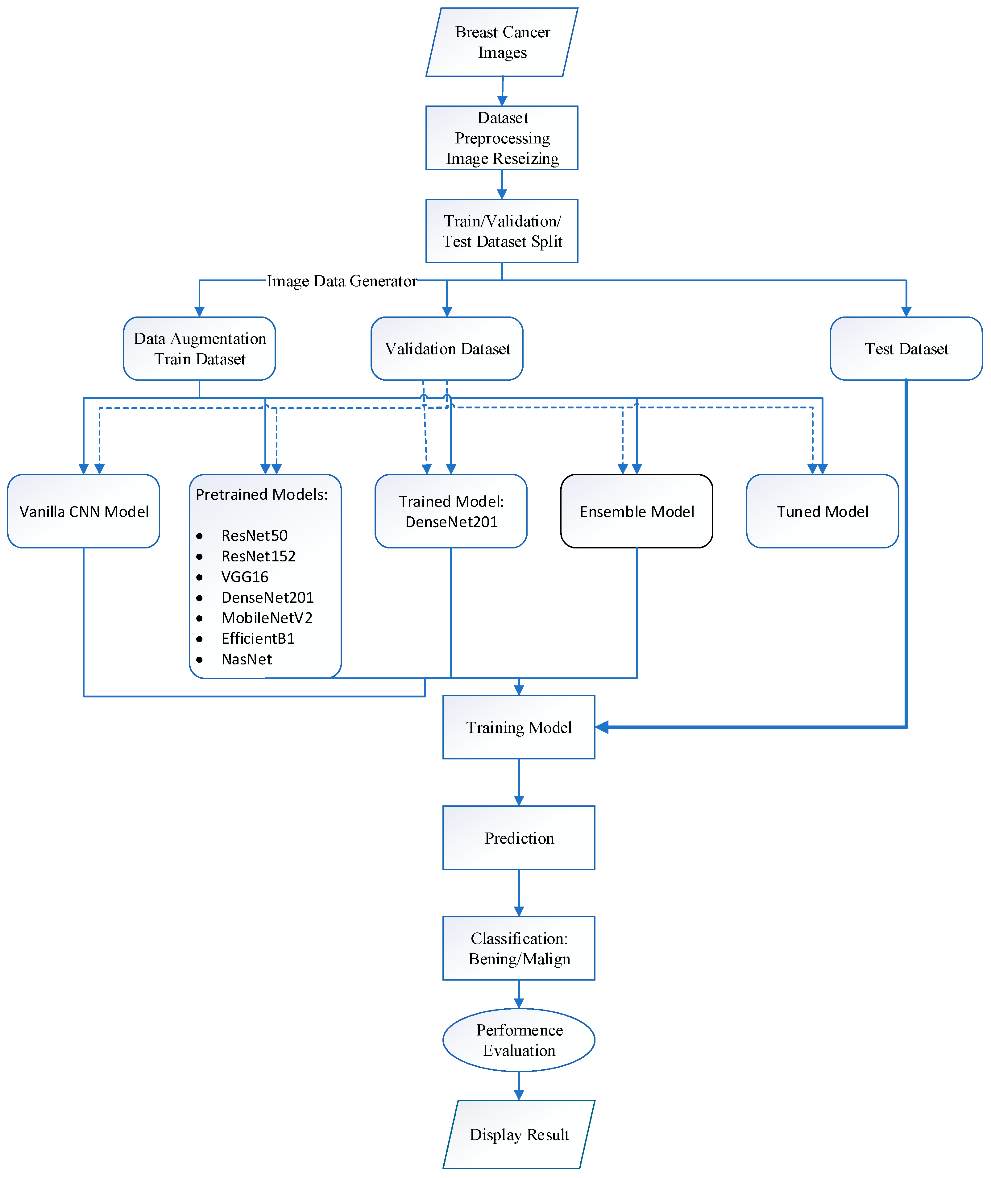
3. Materials and Methods
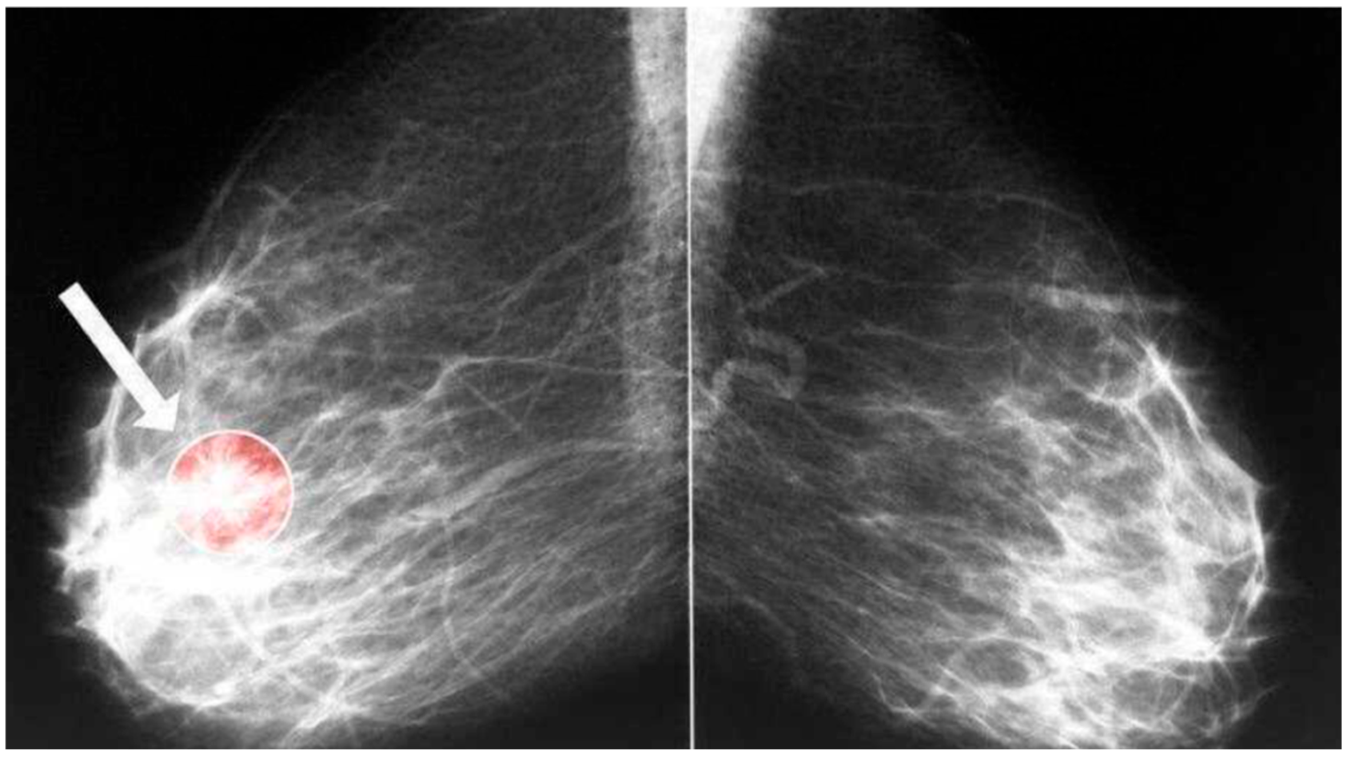
3.1. Datasets
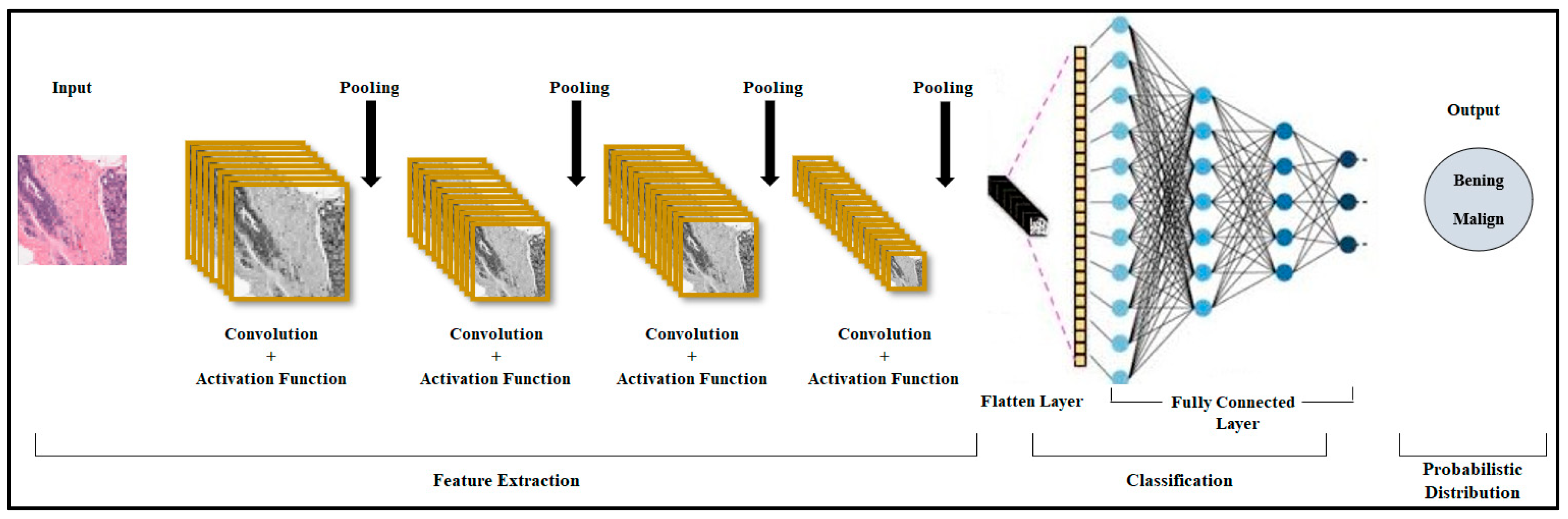
3.2. Convolutional Neural Network (CNN) Model
3.3. ResNet50 Architecture
3.4. ResNet152 Architecture
3.5. VGG16 Architecture
3.6. DenseNet201 Architecture
3.7. MobileNetV2 Architecture
3.8. EfficientNet-B1 Architecture
3.9. Ensemble Model
3.10. Parameter Optimization
3.11. Evaluation Criteria
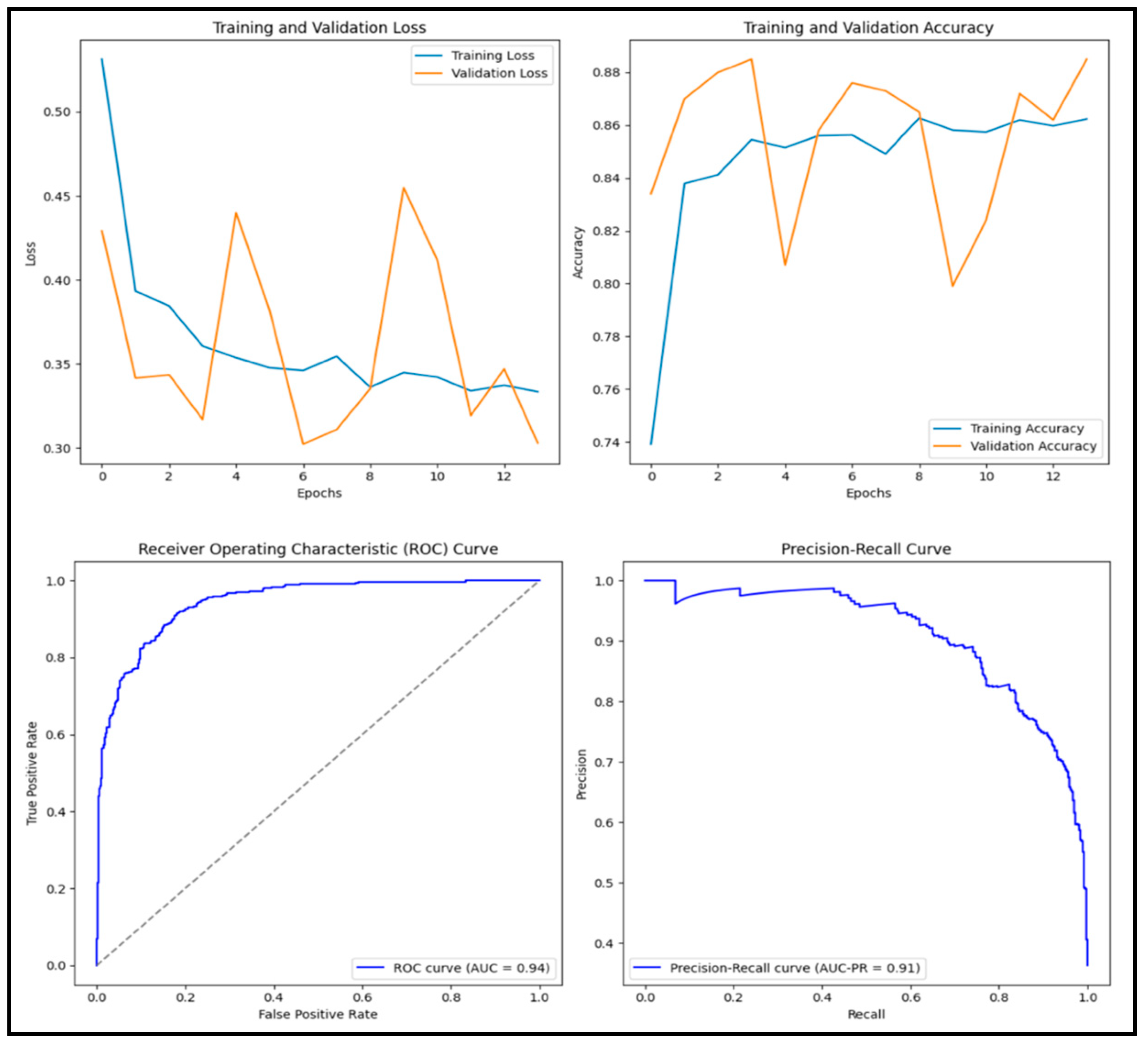
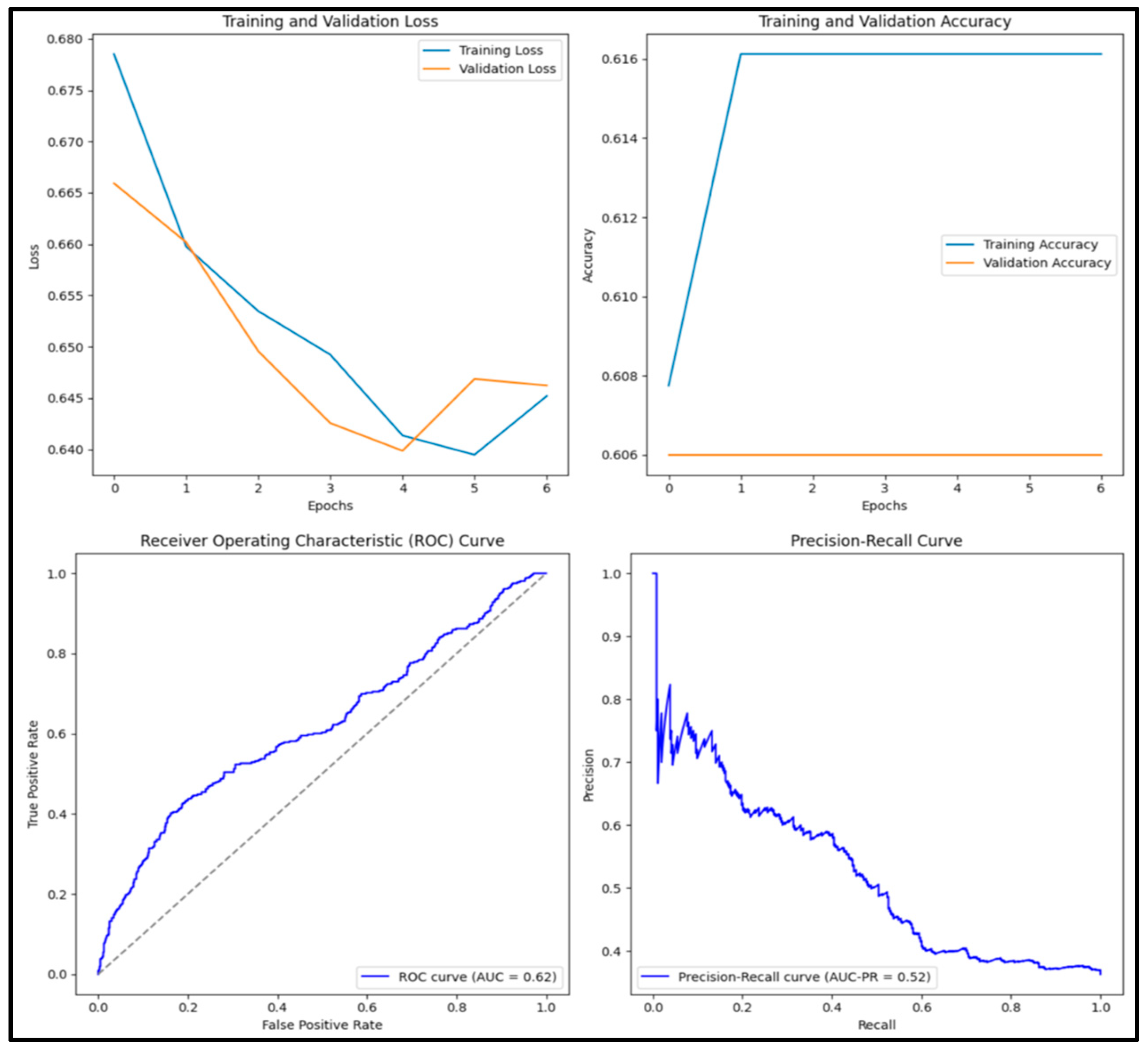
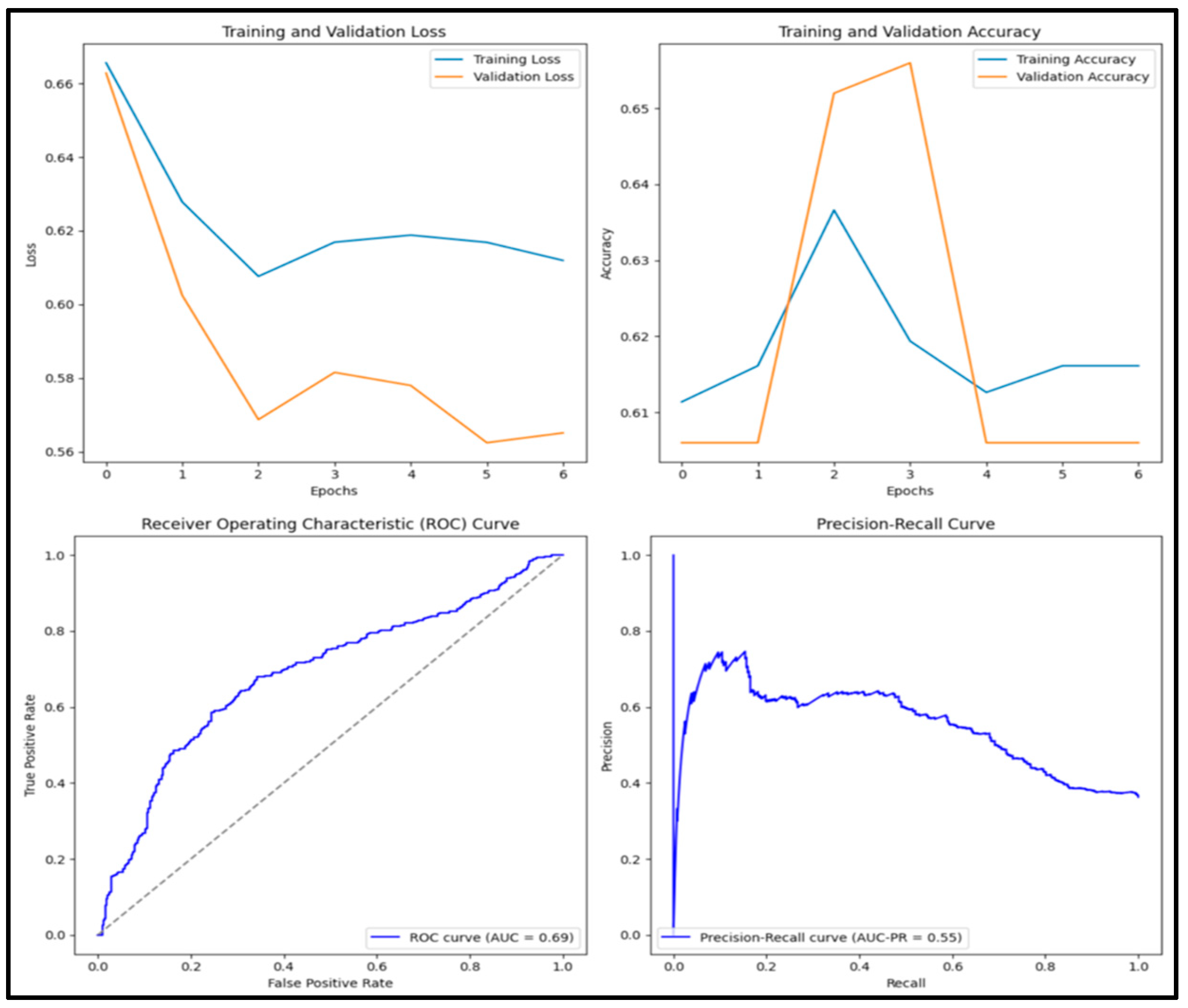
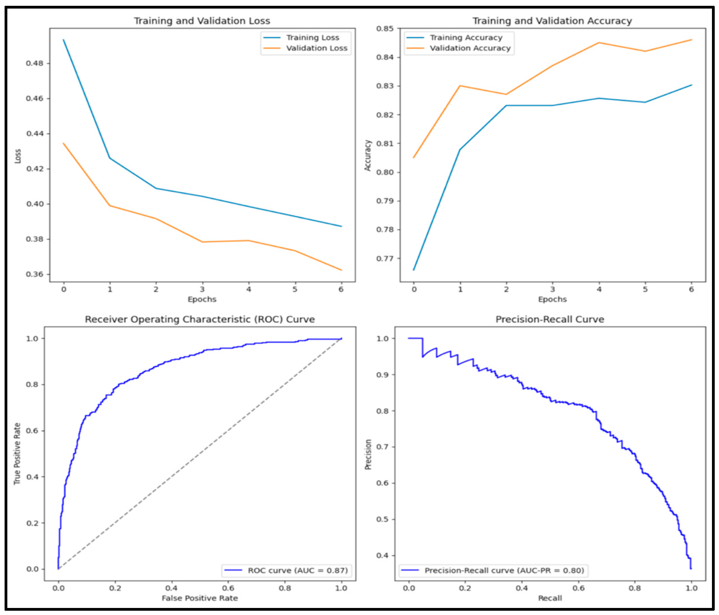
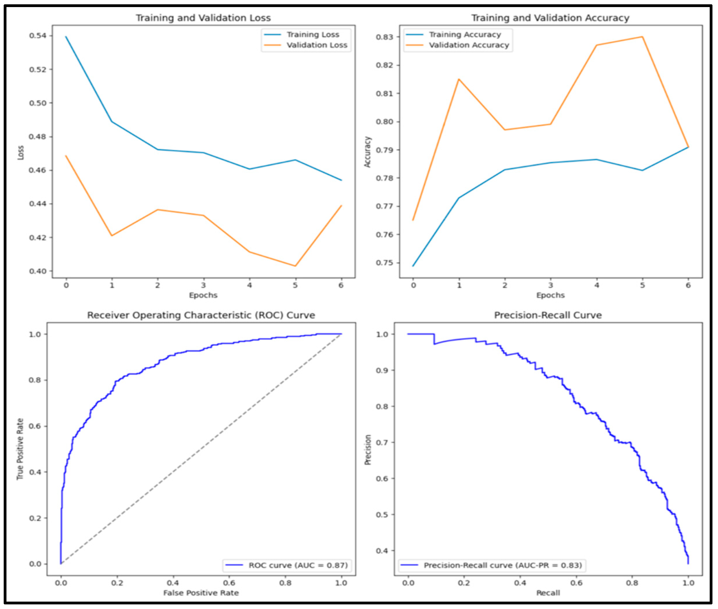
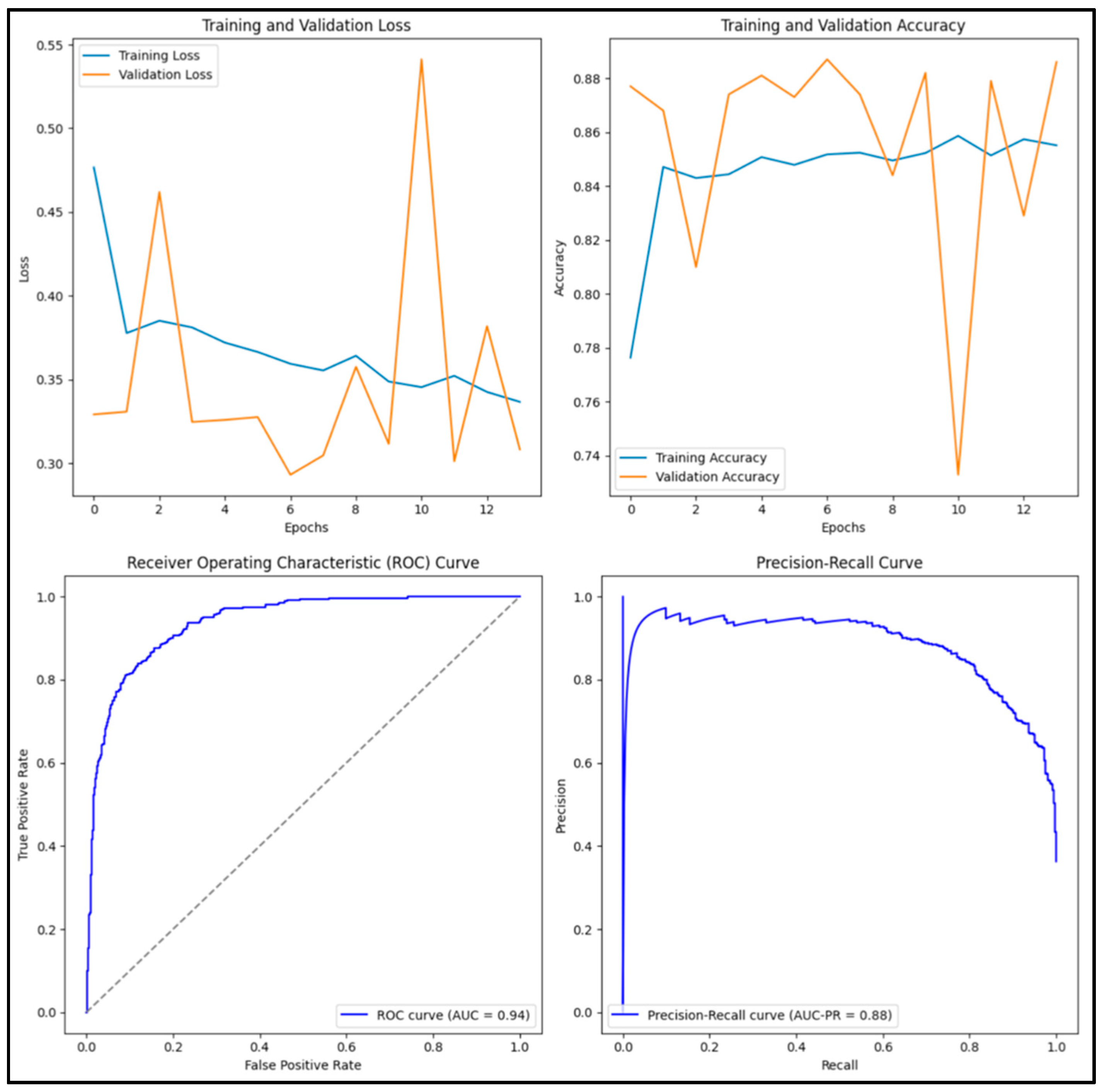
3.12. Experimental Results and Discussion
4. Conclusions
Author Contributions
Funding
Institutional Review Board Statement
Informed Consent Statement
Data Availability Statement
Conflicts of Interest
References
- Arnold, M.; Morgan, E.; Rumgay, H.; Mafra, A.; Singh, D.; Laversanne, M.; Vignat, J.; Gralow, J.R.; Cardoso, F.; Siesling, S.; et al. Current and future burden of breast cancer: Global statistics for 2020 and 2040. Breast 2022, 66, 15–23. [Google Scholar] [CrossRef]
- Litjens, G.; Kooi, T.; Bejnordi, B.E.; Setio, A.A.A.; Ciompi, F.; Ghafoorian, M.; van der Laak, J.A.W.M.; van Ginneken, B.; Sánchez, C.I. A survey on deep learning in medical image analysis. Med. Image Anal. 2017, 42, 60–88. [Google Scholar] [CrossRef] [PubMed]
- Abunasser, B.S.; Al-Hiealy, M.R.J.; Zaqout, I.S.; Abu-Naser, S.S. Convolution neural network for breast cancer detection and classification using deep learning. Asian Pac. J. Cancer Prev. APJCP 2023, 24, 531. [Google Scholar] [CrossRef] [PubMed]
- Güler, M.; Namlı, E. Brain Tumor Detection with Deep Learning Methods’ Classifier Optimization Using Medical Images. Appl. Sci. 2024, 14, 642. [Google Scholar] [CrossRef]
- Kahou, S.E.; Bouthillier, X.; Lamblin, P.; Gulcehre, C.; Michalski, V.; Konda, K.; Jean, S.; Froumenty, P.; Dauphin, Y.; Boulanger-Lewandowski, N.; et al. Emonets: Multimodal deep learning approaches for emotion recognition in video. J. Multimodal User Interfaces 2016, 10, 99–111. [Google Scholar] [CrossRef]
- Subramanian, A.S.; Weng, C.; Watanabe, S.; Yu, M.; Yu, D. Deep learning based multi-source localization with source splitting and its effectiveness in multi-talker speech recognition. Comput. Speech Lang. 2022, 75, 101360. [Google Scholar] [CrossRef]
- Bachute, M.R.; Subhedar, J.M. Autonomous driving architectures: Insights of machine learning and deep learning algorithms. Mach. Learn. Appl. 2021, 6, 100164. [Google Scholar] [CrossRef]
- Khan, A.; Sohail, A.; Zahoora, U.; Qureshi, A.S. A survey of the recent architectures of deep convolutional neural networks. Artif. Intell. Rev. 2020, 53, 5455–5516. [Google Scholar] [CrossRef]
- Nirthika, R.; Manivannan, S.; Ramanan, A.; Wang, R. Pooling in convolutional neural networks for medical image analysis: A survey and an empirical study. Neural Comput. Appl. 2022, 34, 5321–5347. [Google Scholar] [CrossRef]
- Shah, A.; Shah, M.; Pandya, A.; Sushra, R.; Mehta, M.; Patel, K.; Patel, K. A comprehensive study on skin cancer detection using artificial neural network (ANN) and convolutional neural network (CNN). Clin. Ehealth 2023, 6, 76–84. [Google Scholar] [CrossRef]
- Tayal, A.; Gupta, J.; Solanki, A.; Bisht, K.; Nayyar, A.; Masud, M. DL-CNN-based approach with image processing techniques for diagnosis of retinal diseases. Multimed. Syst. 2022, 28, 1417–1438. [Google Scholar] [CrossRef]
- Khuriwal, N.; Mishra, N. Breast cancer diagnosis using deep learning algorithm. In Proceedings of the 2018 International Conference on Advances in Computing, Communication Control and Networking (ICACCCN), Greater Noida, India, 12–13 October 2018; pp. 98–103. [Google Scholar]
- Arefan, D.; Mohamed, A.A.; Berg, W.A.; Zuley, M.L.; Sumkin, J.H.; Wu, S. Deep learning modeling using normal mammograms for predicting breast cancer risk. Med. Phys. 2020, 47, 110–118. [Google Scholar] [CrossRef]
- Mahmood, T.; Li, J.; Pei, Y.; Akhtar, F.; Imran, A.; Rehman, K.U. A brief survey on breast cancer diagnostic with deep learning schemes using multi-image modalities. IEEE Access 2020, 8, 165779–165809. [Google Scholar] [CrossRef]
- Yadavendra; Chand, S. A comparative study of breast cancer tumor classification by classical machine learning methods and deep learning method. Mach. Vis. Appl. 2020, 31, 46. [Google Scholar] [CrossRef]
- Zheng, J.; Lin, D.; Gao, Z.; Wang, S.; He, M.; Fan, J. Deep learning assisted efficient AdaBoost algorithm for breast cancer detection and early diagnosis. IEEE Access 2020, 8, 96946–96954. [Google Scholar] [CrossRef]
- Al Khatib, S.K.; Naous, T.; Shubair, R.M.; El Misilmani, H.M. A deep learning framework for breast tumor detection and localization from microwave imaging data. In Proceedings of the 2021 28th IEEE International Conference on Electronics, Circuits, and Systems (ICECS), Dubai, United Arab Emirates, 28 November–1 December 2021; pp. 1–4. [Google Scholar]
- Zhang, Z.; Li, Y.; Wu, W.; Chen, H.; Cheng, L.; Wang, S. Tumor detection using deep learning method in automated breast ultrasound. Biomed. Signal Process. Control 2021, 68, 102677. [Google Scholar] [CrossRef]
- Alkhaleefah, M.; Tan, T.H.; Chang, C.H.; Wang, T.C.; Ma, S.C.; Chang, L.; Chang, Y.L. Connected-segNets: A deep learning model for breast tumor segmentation from X-ray images. Cancers 2022, 14, 4030. [Google Scholar] [CrossRef] [PubMed]
- Cho, S.W.; Baek, N.R.; Park, K.R. Deep Learning-based Multi-stage segmentation method using ultrasound images for breast cancer diagnosis. J. King Saud Univ.-Comput. Inf. Sci. 2022, 34, 10273–10292. [Google Scholar] [CrossRef]
- Jasti, V.D.P.; Zamani, A.S.; Arumugam, K.; Naved, M.; Pallathadka, H.; Sammy, F.; Raghuvanshi, A.; Kaliyaperumal, K.; Reddy, G.T. Computational technique based on machine learning and image processing for medical image analysis of breast cancer diagnosis. Secur. Commun. Netw. 2022, 2022, 1918379. [Google Scholar] [CrossRef]
- Li, Y.; Gu, H.; Wang, H.; Qin, P.; Wang, J. BUSnet: A deep learning model of breast tumor lesion detection for ultrasound images. Front. Oncol. 2022, 12, 848271. [Google Scholar] [CrossRef]
- Afrin, H.; Larson, N.B.; Fatemi, M.; Alizad, A. Deep learning in different ultrasound methods for breast cancer, from diagnosis to prognosis: Current trends, challenges, and an analysis. Cancers 2023, 15, 3139. [Google Scholar] [CrossRef] [PubMed]
- Avcı, H.; Karakaya, J. A novel medical image enhancement algorithm for breast cancer detection on mammography images using machine learning. Diagnostics 2023, 13, 348. [Google Scholar] [CrossRef]
- Dar, M.F.; Ganivada, A. Efficientu-net: A novel deep learning method for breast tumor segmentation and classification in ultrasound images. Neural Process. Lett. 2023, 55, 10439–10462. [Google Scholar] [CrossRef]
- Humayun, M.; Khalil, M.I.; Almuayqil, S.N.; Jhanjhi, N.Z. Framework for detecting breast cancer risk presence using deep learning. Electronics 2023, 12, 403. [Google Scholar] [CrossRef]
- Khalid, A.; Mehmood, A.; Alabrah, A.; Alkhamees, B.F.; Amin, F.; AlSalman, H.; Choi, G.S. Breast cancer detection and prevention using machine learning. Diagnostics 2023, 13, 3113. [Google Scholar] [CrossRef]
- Kutluer, N.; Solmaz, O.A.; Yamacli, V.; Eristi, B.; Eristi, H. Classification of breast tumors by using a novel approach based on deep learning methods and feature selection. Breast Cancer Res. Treat. 2023, 200, 183–192. [Google Scholar] [CrossRef] [PubMed]
- Maleki, A.; Raahemi, M.; Nasiri, H. Breast cancer diagnosis from histopathology images using deep neural network and XGBoost. Biomed. Signal Process. Control 2023, 86, 105152. [Google Scholar] [CrossRef]
- Raza, A.; Ullah, N.; Khan, J.A.; Assam, M.; Guzzo, A.; Aljuaid, H. DeepBreastCancerNet: A novel deep learning model for breast cancer detection using ultrasound images. Appl. Sci. 2023, 13, 2082. [Google Scholar] [CrossRef]
- Zakareya, S.; Izadkhah, H.; Karimpour, J. A new deep-learning-based model for breast cancer diagnosis from medical images. Diagnostics 2023, 13, 1944. [Google Scholar] [CrossRef]
- Zhang, Q.; Cai, G.; Cai, M.; Qian, J.; Song, T. Deep Learning Model Aids Breast Cancer Detection. Front. Comput. Intell. Syst. 2023, 6, 99–102. [Google Scholar] [CrossRef]
- Alashban, Y. Breast cancer detection and classification with digital breast tomosynthesis: A two-stage deep learning approach. Diagn. Interv. Radiol. 2025, 31, 206–214. [Google Scholar] [CrossRef] [PubMed]
- Klanecek, Z.; Wang, Y.-K.; Wagner, T.; Cockmartin, L.; Marshall, N.; Schott, B.; Deatsch, A.; Studen, A.; Hertl, K.; Jarm, K.; et al. Longitudinal interpretability of deep learning-based breast cancer risk prediction model: Comparison of different attribution methods. In Proceedings of the 17th International Workshop on Breast Imaging, Chicago, IL, USA, 29 May 2024; Volume 13174, pp. 478–484. [Google Scholar]
- Sahu, A.; Das, P.K.; Meher, S. An efficient deep learning scheme to detect breast cancer using mammogram and ultrasound breast images. Biomed. Signal Process. Control 2024, 87, 105377. [Google Scholar] [CrossRef]
- Abdusalomov, A.B.; Mukhiddinov, M.; Whangbo, T.K. Brain tumor detection based on deep learning approaches and magnetic resonance imaging. Cancers 2023, 15, 4172. [Google Scholar] [CrossRef]
- Kumar, V.; Joshi, K.; Kanti, P.; Reshi, J.S.; Rawat, G.; Kumar, A. Brain tumor diagnosis using image fusion and deep learning. In Proceedings of the 2023 International Conference on Sustainable Computing and Data Communication Systems (ICSCDS), Erode, India, 23–25 March 2023; pp. 1658–1662. [Google Scholar]
- Khan, M.F.; Iftikhar, A.; Anwar, H.; Ramay, S.A. Brain tumor segmentation and classification using optimized deep learning. J. Comput. Biomed. Inform. 2024, 7, 632–640. [Google Scholar]
- Ghosh, H.; Rahat, I.S.; Mohanty, S.N.; Ravindra, J.V.R.; Sobur, A. A Study on the Application of Machine Learning and Deep Learning Techniques for Skin Cancer Detection. Int. J. Comput. Syst. Eng. 2024, 18, 51–59. [Google Scholar]
- Khan, A.A.; Arslan, M.; Tanzil, A.; Bhatty, R.A.; Khalid, M.A.U.; Khan, A.H. Classification of colon cancer using deep learning techniques on histopathological images. Migr. Lett. 2024, 21 (Suppl. S11), 449–463. [Google Scholar]
- Wankhade, S.; Vigneshwari, S. A novel hybrid deep learning method for early detection of lung cancer using neural networks. Healthc. Anal. 2023, 3, 100195. [Google Scholar] [CrossRef]
- Breast Tumor Dataset-Kaggle. Predict IDC in Breast Cancer Histology Images. Available online: https://www.kaggle.com/code/paultimothymooney/predict-idc-in-breast-cancer-histology-images/notebook (accessed on 7 July 2025).
- Montesinos López, O.A.; Montesinos López, A.; Crossa, J. Convolutional neural networks. In Multivariate Statistical Machine Learning Methods for Genomic Prediction; Springer International Publishing: Cham, Switzerland, 2022; pp. 533–577. [Google Scholar]
- Mukti, I.Z.; Biswas, D. Transfer learning-based plant diseases detection using ResNet50. In Proceedings of the 2019 4th International Conference on Electrical Information and Communication Technology (EICT), Khulna, Bangladesh, 20–22 December 2019; pp. 1–6. [Google Scholar]
- Yu, Y.; Lin, H.; Meng, J.; Wei, X.; Guo, H.; Zhao, Z. Deep transfer learning for modality classification of medical images. Information 2017, 8, 91. [Google Scholar] [CrossRef]
- Zhang, L.; Li, H.; Zhu, R.; Du, P. An infrared and visible image fusion algorithm based on ResNet-152. Multimed. Tools Appl. 2022, 81, 9277–9287. [Google Scholar] [CrossRef]
- Burra, L.R.; Bonam, J.; Tumuluru, P.; Narendra Kumar Rao, B. Fine-tuning for transfer learning of ResNet152 for disease identification in tomato leaves. In Intelligent Computing and Applications: Proceedings of ICDIC 2020; Springer Nature: Singapore, 2022; pp. 295–302. [Google Scholar]
- Theckedath, D.; Sedamkar, R.R. Detecting affect states using VGG16, ResNet50 and SE-ResNet50 networks. SN Comput. Sci. 2020, 1, 79. [Google Scholar] [CrossRef]
- Huang, G.; Chen, D.; Li, T.; Wu, F.; Van Der Maaten, L.; Weinberger, K.Q. Multi-scale dense networks for resource efficient image classification. arXiv 2018, arXiv:1703.09844. [Google Scholar]
- Tan, M.; Le, Q.E. Rethinking model scaling for convolutional neural networks. arXiv 2019, arXiv:1905.11946. [Google Scholar]
- Zoph, B.; Vasudevan, V.; Shlens, J.; Le, Q.V. Learning transferable architectures for scalable image recognition. In Proceedings of the IEEE Conference on Computer Vision and Pattern Recognition, Salt Lake City, UT, USA, 18–23 June 2018; pp. 8697–8710. [Google Scholar]
- Ganaie, M.A.; Hu, M.; Malik, A.K.; Tanveer, M.; Suganthan, P.N. Ensemble deep learning: A review. Eng. Appl. Artif. Intell. 2022, 115, 105151. [Google Scholar] [CrossRef]
- Tan, M.; Chen, B.; Pang, R.; Vasudevan, V.; Sandler, M.; Howard, A.; Le, Q.V. Mnasnet: Platform-aware neural architecture search for mobile. In Proceedings of the IEEE Conference on Computer Vision and Pattern Recognition, Long Beach, CA, USA, 15–20 June 2019; pp. 2820–2828. [Google Scholar]
- Duchi, J.; Hazan, E.; Singer, Y. Adaptive subgradient methods for online learning and stochastic optimization. J. Mach. Learn. Res. 2011, 12, 2121–2159. [Google Scholar]
- Hossin, M.; Sulaiman, M.N. A Review on Evaluation Metrics for Data Classification Evaluations. Int. J. Data Min. Knowl. Manag. Process 2015, 5, 1–11. [Google Scholar]


| Predicted Value | |||
|---|---|---|---|
| Positive | Negative | ||
| Actual Value | Positive | True positive (TP) | False negative (FN) |
| Negative | False positive (FP) | True negative (TN) | |
| Model | Accuracy | Precision | Recall | F1 | AUC |
|---|---|---|---|---|---|
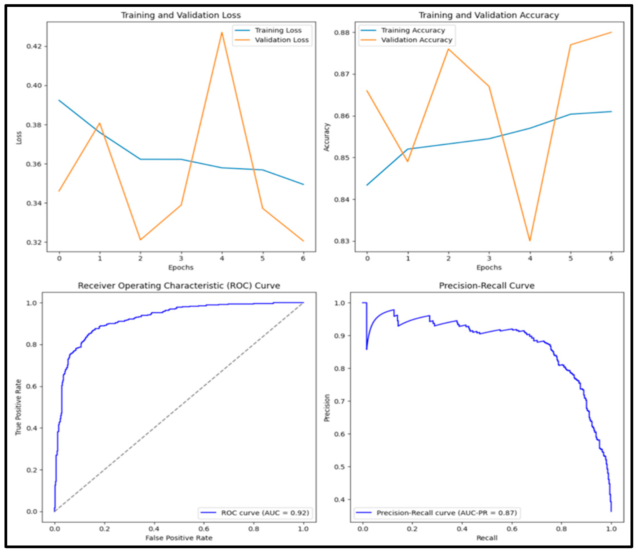
| Vanilla | 0.854 | 0.788 | 0.857 | 0.821 | 0.937 |
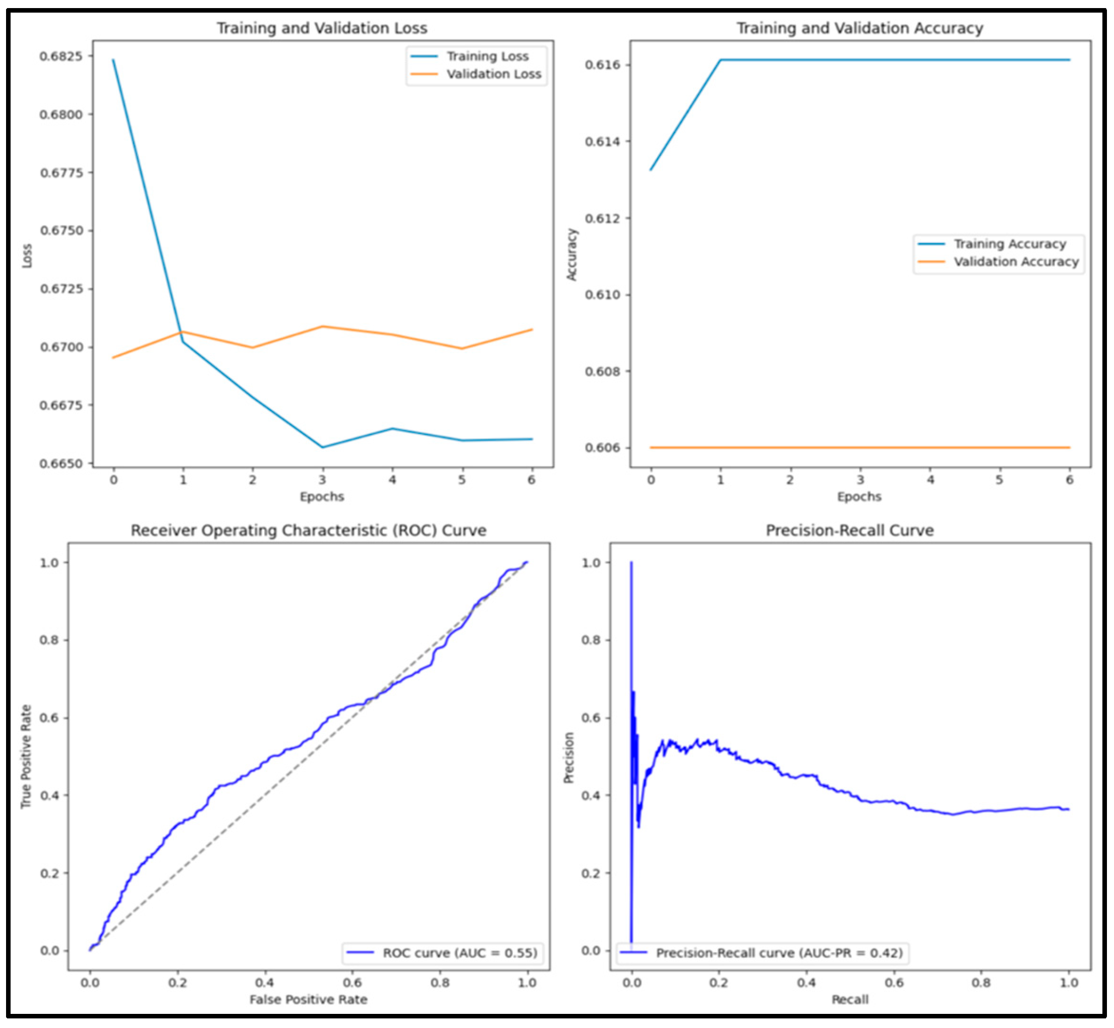
| ResNet50 | 0.609 | 0 | 0 | 0 | 0.602 |
| ResNet152 | 0.609 | 0 | 0 | 0 | 0.752 |
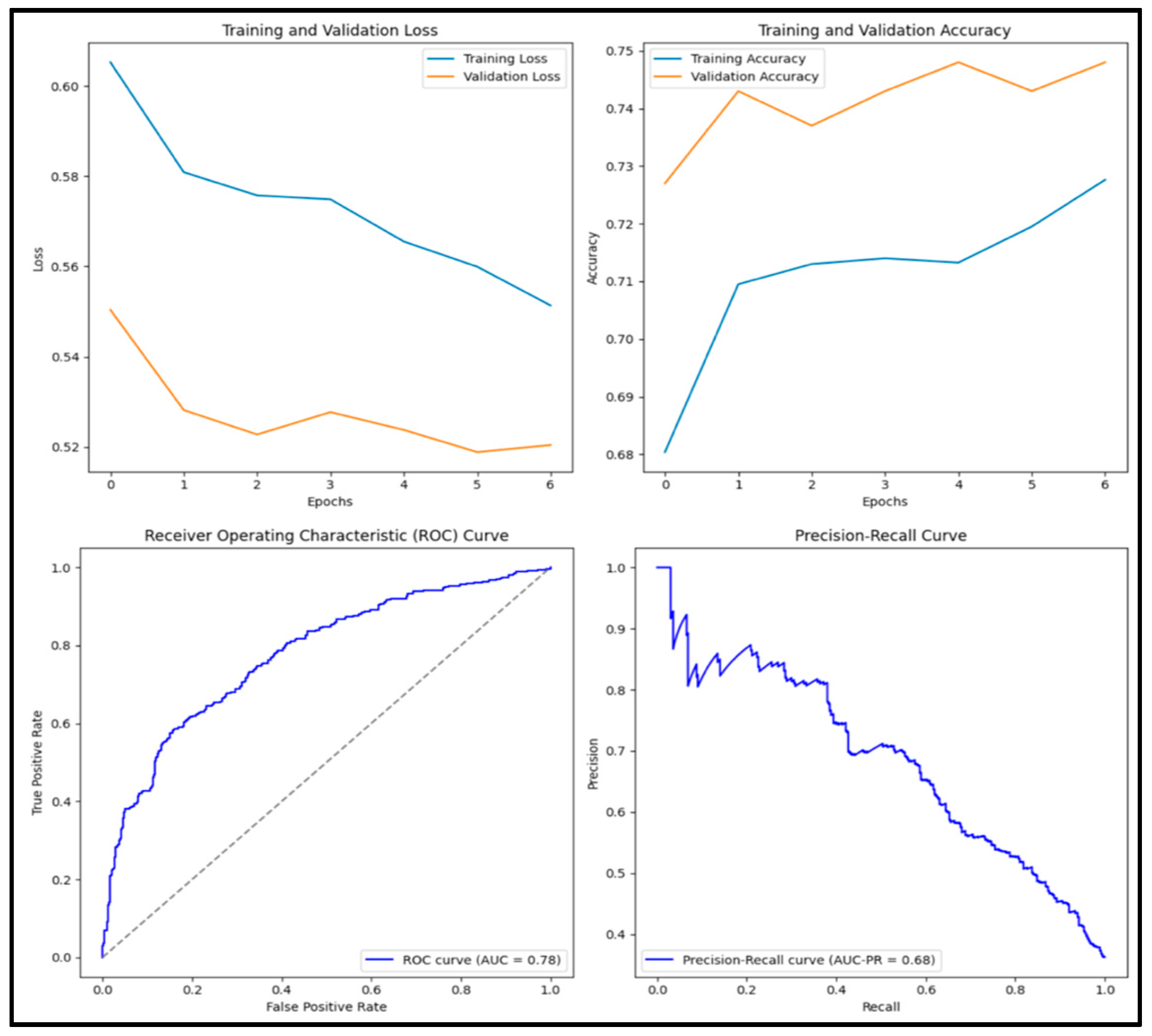
| VGG16 | 0.794 | 0.790 | 0.645 | 0.710 | 0.853 |
| DenseNet152 | 0.818 | 0.785 | 0.737 | 0.760 | 0.882 |
| MobileNetv2 | 0.773 | 0.693 | 0.755 | 0.722 | 0.856 |
| EfficientB1 | 0.609 | 0 | 0 | 0 | 0.472 |
| NasNet | 0.705 | 0.648 | 0.537 | 0.587 | 0.762 |
| DenseNet201 | 0.894 | 0.882 | 0.841 | 0.861 | 0.958 |
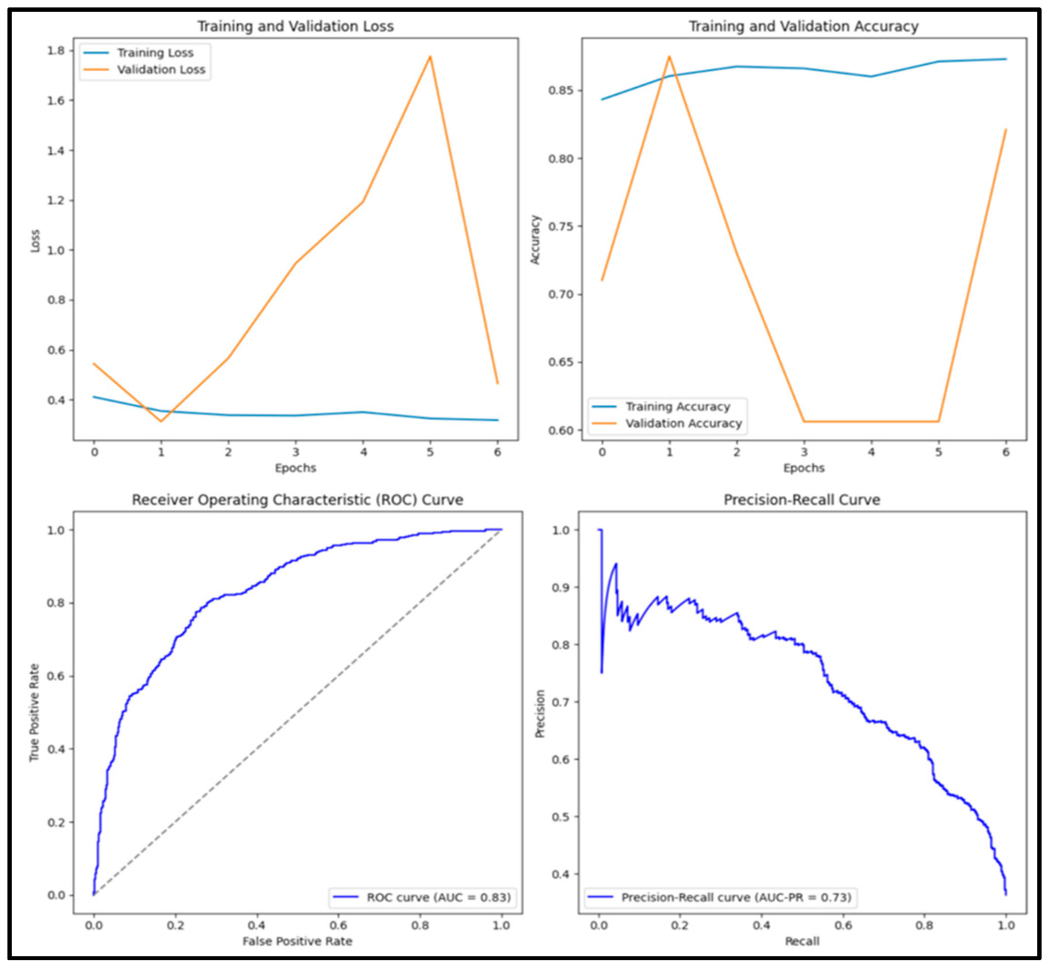
| Ensemble | 0.822 | 0.728 | 0.870 | 0.793 | 0.917 |
| Tuned Model | 0.820 | 0.762 | 0.785 | 0.773 | 0.885 |
Disclaimer/Publisher’s Note: The statements, opinions and data contained in all publications are solely those of the individual author(s) and contributor(s) and not of MDPI and/or the editor(s). MDPI and/or the editor(s) disclaim responsibility for any injury to people or property resulting from any ideas, methods, instructions or products referred to in the content. |
© 2025 by the authors. Licensee MDPI, Basel, Switzerland. This article is an open access article distributed under the terms and conditions of the Creative Commons Attribution (CC BY) license (https://creativecommons.org/licenses/by/4.0/).
Share and Cite
Güler, M.; Sart, G.; Algorabi, Ö.; Adıguzel Tuylu, A.N.; Türkan, Y.S. Breast Cancer Classification with Various Optimized Deep Learning Methods. Diagnostics 2025, 15, 1751. https://doi.org/10.3390/diagnostics15141751
Güler M, Sart G, Algorabi Ö, Adıguzel Tuylu AN, Türkan YS. Breast Cancer Classification with Various Optimized Deep Learning Methods. Diagnostics. 2025; 15(14):1751. https://doi.org/10.3390/diagnostics15141751
Chicago/Turabian StyleGüler, Mustafa, Gamze Sart, Ömer Algorabi, Ayse Nur Adıguzel Tuylu, and Yusuf Sait Türkan. 2025. "Breast Cancer Classification with Various Optimized Deep Learning Methods" Diagnostics 15, no. 14: 1751. https://doi.org/10.3390/diagnostics15141751
APA StyleGüler, M., Sart, G., Algorabi, Ö., Adıguzel Tuylu, A. N., & Türkan, Y. S. (2025). Breast Cancer Classification with Various Optimized Deep Learning Methods. Diagnostics, 15(14), 1751. https://doi.org/10.3390/diagnostics15141751