

Magnifying Networks for Histopathological Images with Billions of Pixels


Abstract
1. Introduction
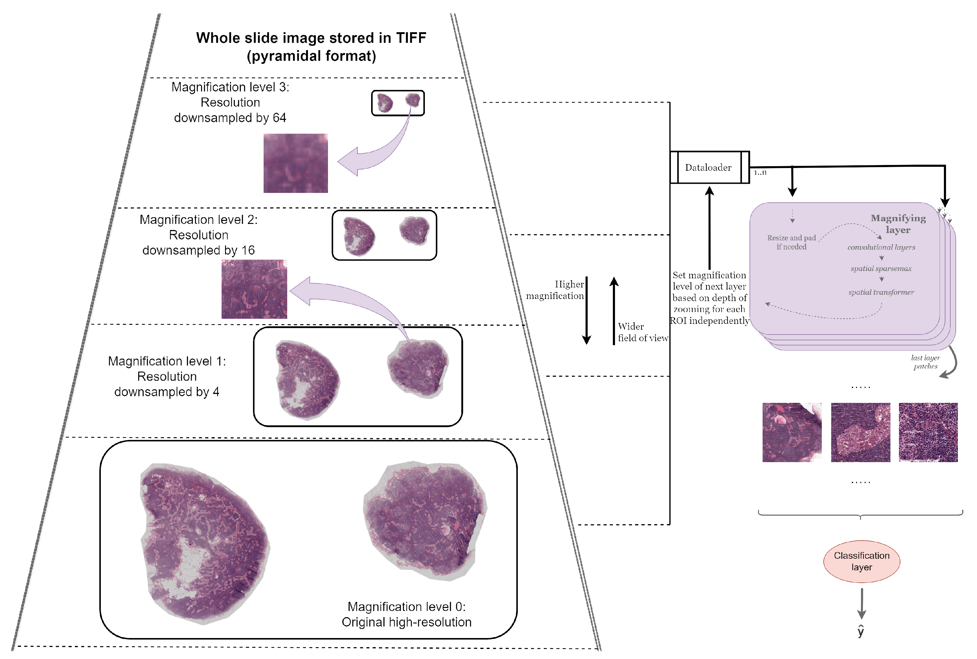
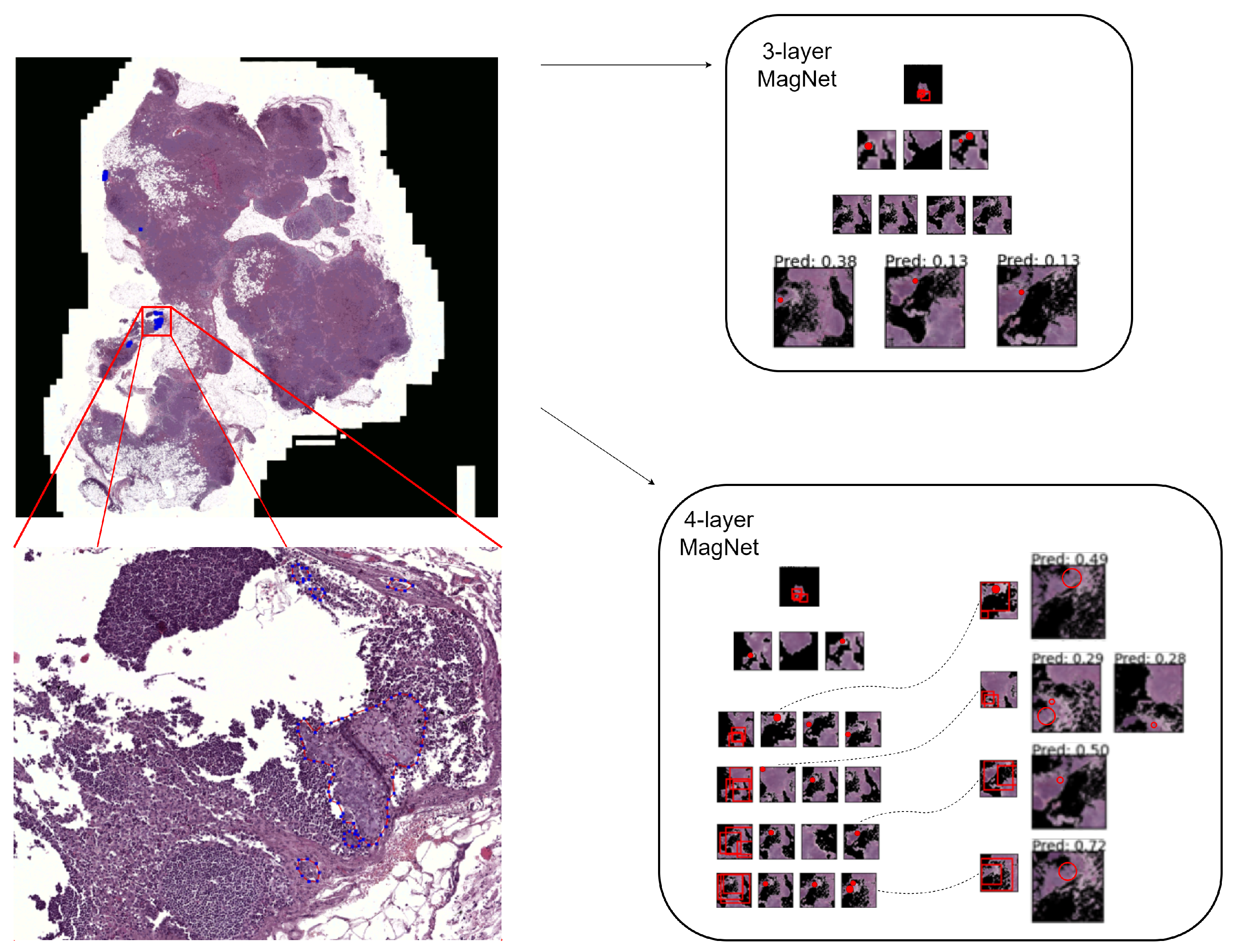
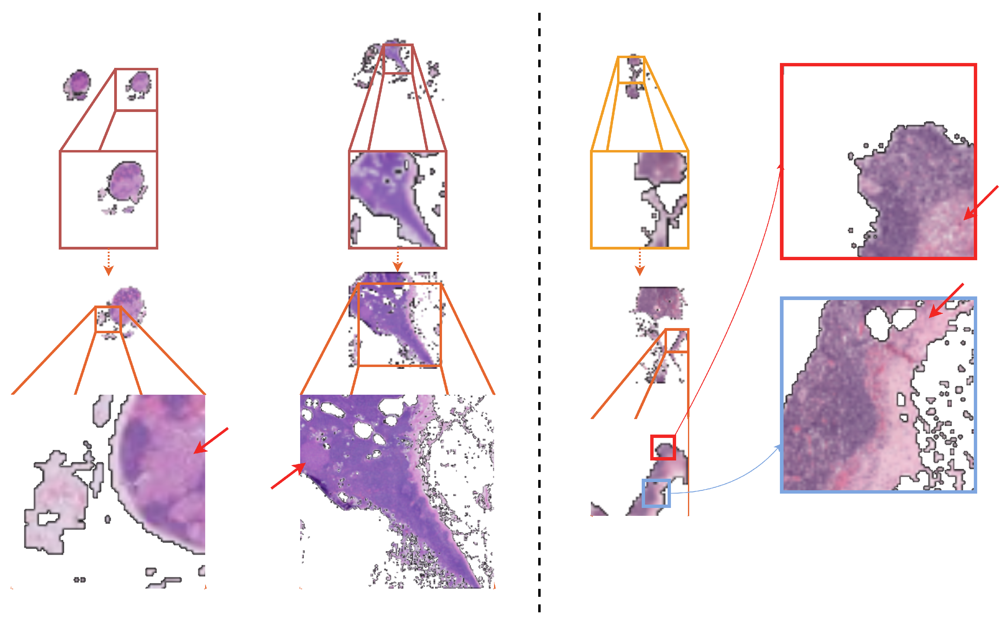
- In the context of the WSI classification of metastases, we propose the possibility of identifying and magnifying ROIs starting from a very-low-resolution downsampled version of the WSI (three channels; pixels), and, experimentally, we show that recursively identifying and magnifying regions of interest (ROI) allows for the extraction of informative areas across magnification levels.
- Without leaving the weakly supervised paradigm, we explore nested attention using the spatial transformer module for gigapixel image analysis.
- To the best of our knowledge, this is the first work that automatically learns to select regions that are analyzed at potentially progressively greater magnification levels and, thus, fuses extracted information across scales. As such, the proposed method is able to exploit rich contextual and salient features, overcoming the typical problem of patch-based processing that poorly captures the information that is distributed beyond the patch size.
2. Related Work
2.1. Patch Extraction
2.1.1. Strongly Supervised
2.1.2. Weakly Supervised
2.2. Patch Selection
2.2.1. Attention
2.2.2. Nested Attention
3. Materials and Methods
3.1. Datasets
3.2. Magnifying Networks
3.2.1. Magnifying Layer
Resizing and Padding
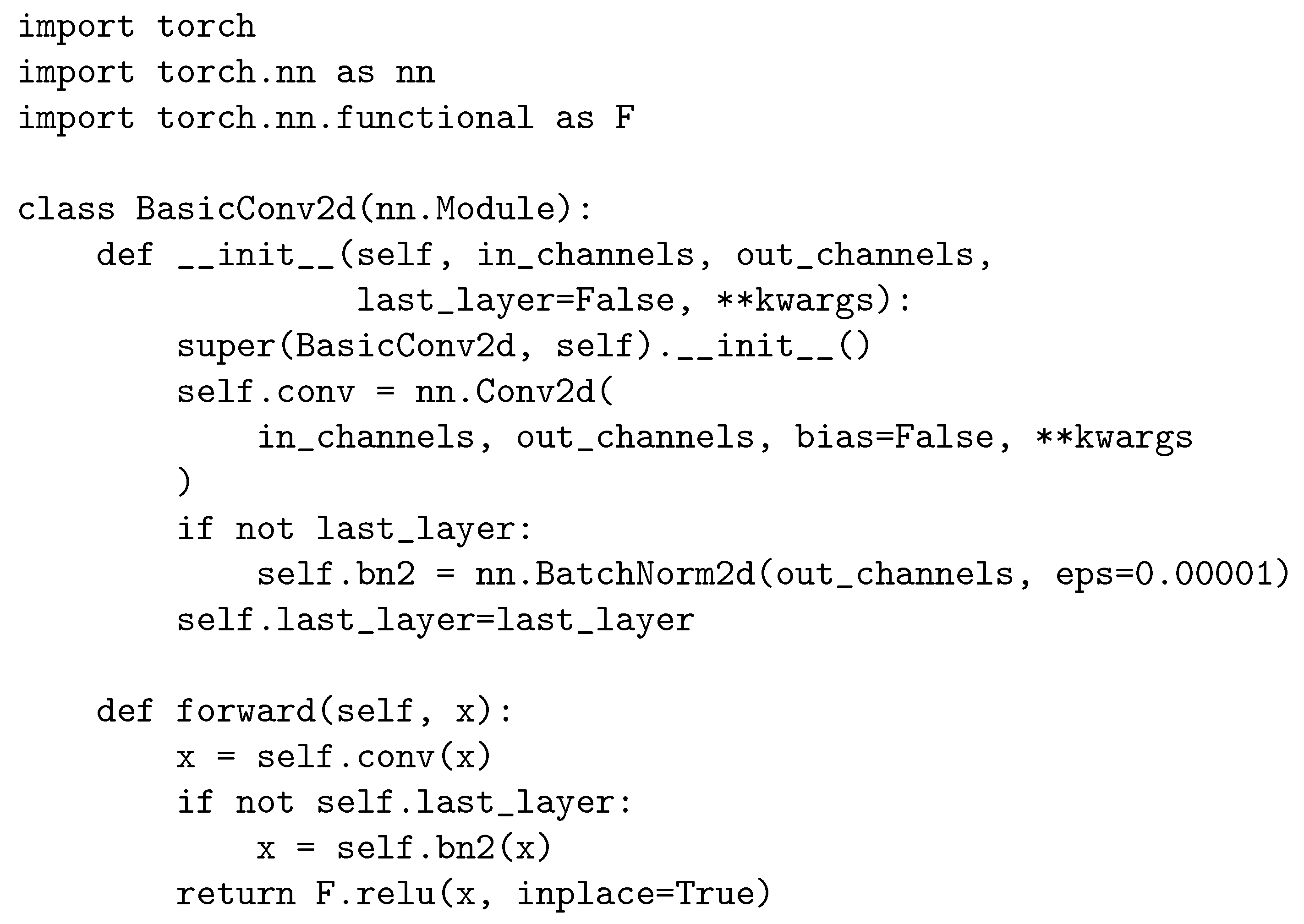
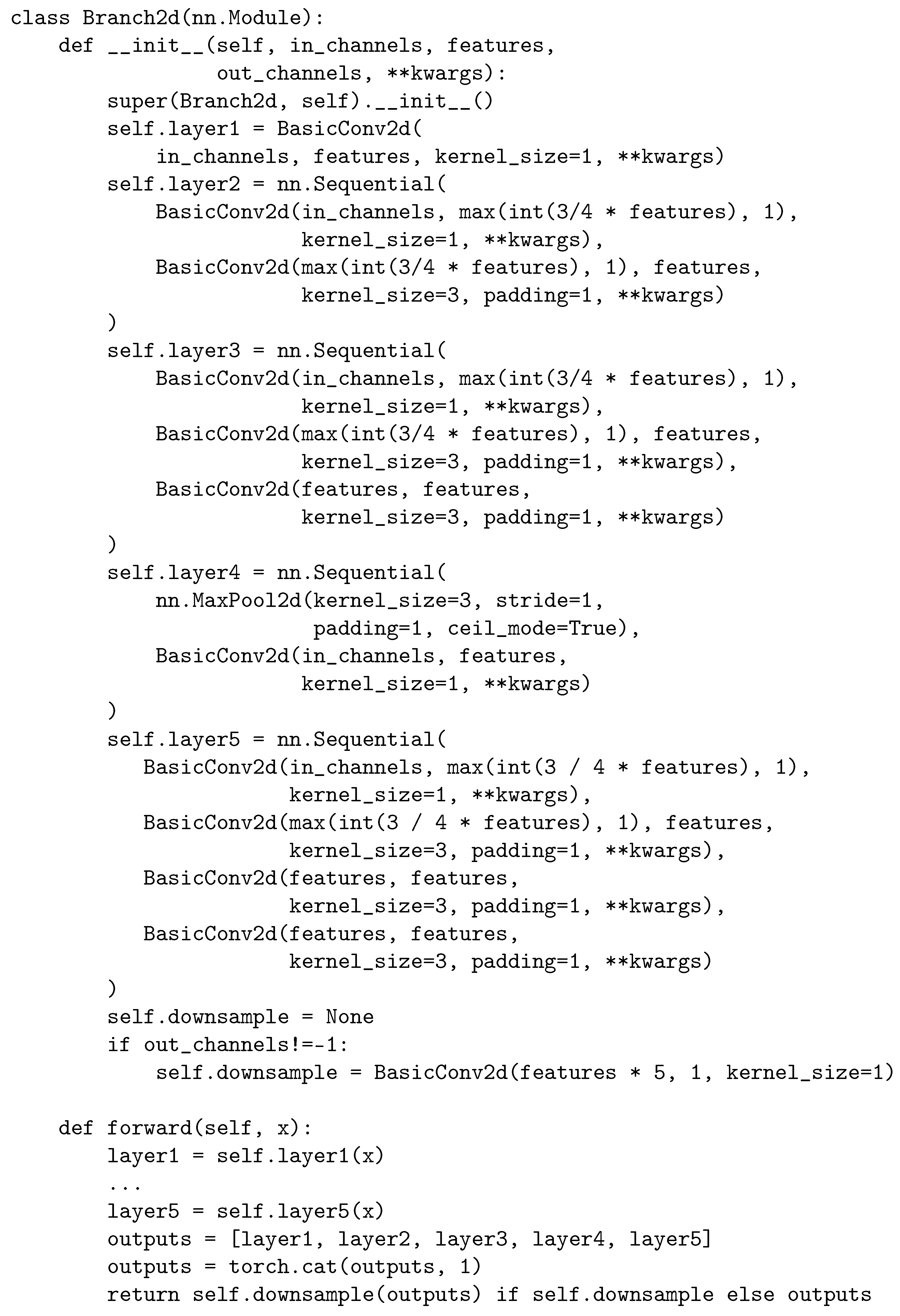
Convolutional Layers
- Conv2D;
- Conv2D⇝ Conv2D;
- Conv2D⇝ Conv2D⇝ Conv2D;
- Conv2D⇝ Conv2D⇝ Conv2D⇝ Conv2D;
- MaxPool⇝ Conv2D.
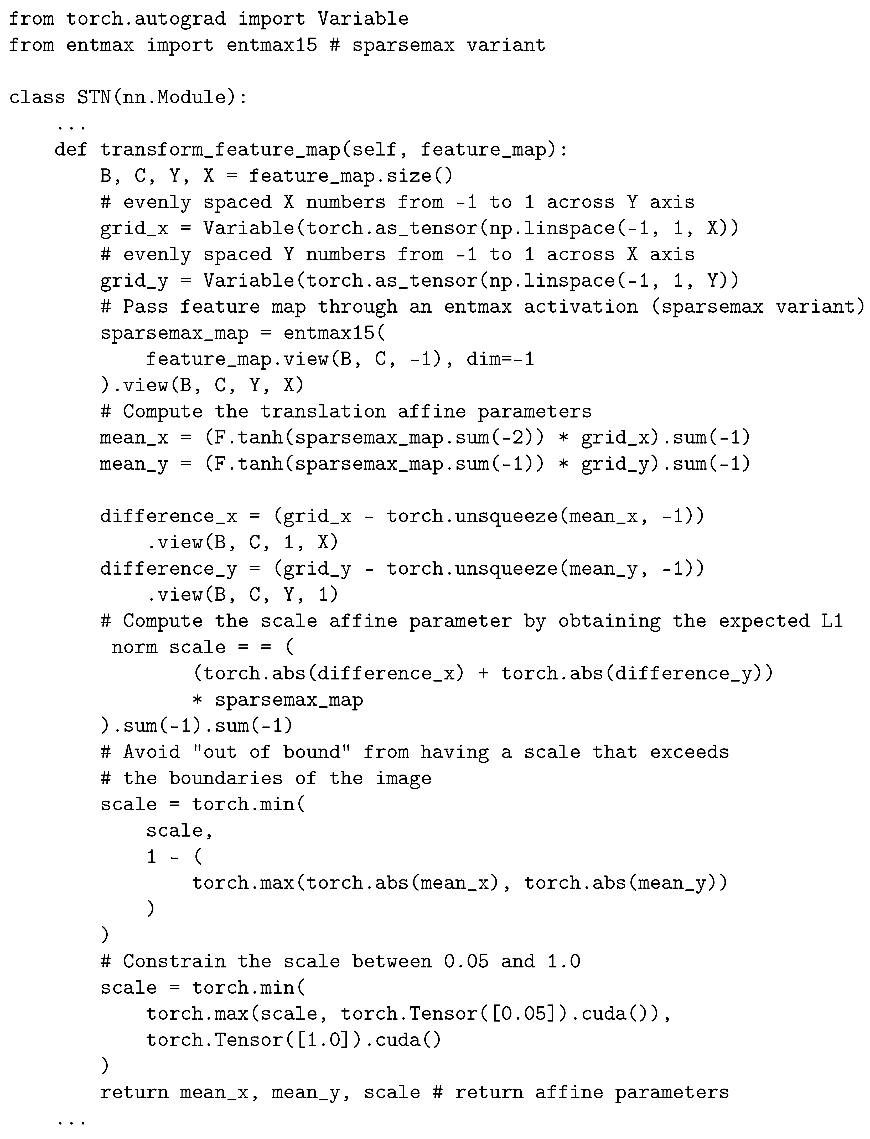
Spatial Transformer
Sampler
Sampling
| Width | Height | WSI resolution | level | |
| ≥25,000 | and | ≥50,000 | pixels | 8 |
| ≥12,500 | or | ≥25,000 | pixels | 7 |
| ≥6250 | or | ≥12,500 | pixels | 6 |
| ≥3125 | or | ≥6250 | pixels | 5 |
| ≥1563 | or | ≥3125 | pixels | 4 |
| ≥782 | or | ≥1563 | 12,500 pixels | 3 |
| ≥391 | or | ≥782 | 12,500 × 25,000 pixels | 2 |
| ≥171 | or | ≥391 | 25,000 × 50,000 pixels | 1 |
| <171 | and | <391 | 50,000 × 100,000 pixels | 0 |
3.2.2. Classification Layer
3.2.3. Auxiliary Classifiers
3.2.4. Configurations
3.3. Evaluation
3.3.1. Data Augmentation
3.3.2. Training
3.3.3. “Frozen” Patch
3.3.4. Loss Functions
4. Results
5. Discussion
Limitations
6. Conclusions
Author Contributions
Funding
Institutional Review Board Statement
Informed Consent Statement
Data Availability Statement
Conflicts of Interest
Appendix A. Implementation Details
Appendix A.1. Convolutional Layers
Appendix A.2. Spatial Transformer
References
- Dimitriou, N.; Arandjelović, O.; Caie, P.D. Deep Learning for Whole Slide Image Analysis: An Overview. Front. Med. 2019, 6, 264. [Google Scholar] [CrossRef]
- Caie, P.D.; Dimitriou, N.; Arandjelović, O. Chapter 8—Precision medicine in digital pathology via image analysis and machine learning. In Artificial Intelligence and Deep Learning in Pathology; Cohen, S., Ed.; Elsevier: Amsterdam, The Netherlands, 2021; pp. 149–173. [Google Scholar] [CrossRef]
- Vaswani, A.; Shazeer, N.; Parmar, N.; Uszkoreit, J.; Jones, L.; Gomez, A.N.; Kaiser, L.u.; Polosukhin, I. Attention is All you Need. In Proceedings of the Advances in Neural Information Processing Systems; Guyon, I., Luxburg, U.V., Bengio, S., Wallach, H., Fergus, R., Vishwanathan, S., Garnett, R., Eds.; Curran Associates, Inc.: New York, NY, USA, 2017; Volume 30. [Google Scholar]
- Bejnordi, B.E.; Veta, M.; Van Diest, P.J.; Van Ginneken, B.; Karssemeijer, N.; Litjens, G.; Van Der Laak, J.A.; Hermsen, M.; Manson, Q.F.; Balkenhol, M.; et al. Diagnostic assessment of deep learning algorithms for detection of lymph node metastases in women with breast cancer. JAMA 2017, 318, 2199–2210. [Google Scholar] [CrossRef] [PubMed]
- Aresta, G.; Araújo, T.; Kwok, S.; Chennamsetty, S.S.; Safwan, M.; Alex, V.; Marami, B.; Prastawa, M.; Chan, M.; Donovan, M.; et al. BACH: Grand Challenge on Breast Cancer Histology Images. arXiv 2018, arXiv:1808.04277. [Google Scholar] [CrossRef] [PubMed]
- Fell, C.; Mohammadi, M.; Morrison, D.; Arandjelović, O.; Syed, S.; Konanahalli, P.; Bell, S.; Bryson, G.; Harrison, D.J.; Harris-Birtill, D. Detection of malignancy in whole slide images of endometrial cancer biopsies using artificial intelligence. PLoS ONE 2023, 18, e0282577. [Google Scholar] [CrossRef] [PubMed]
- Simonyan, K.; Zisserman, A. Very Deep Convolutional Networks for Large-Scale Image Recognition. arXiv 2014, arXiv:1409.1556. [Google Scholar]
- He, K.; Zhang, X.; Ren, S.; Sun, J. Deep Residual Learning for Image Recognition. In Proceedings of the 2016 IEEE Conference on Computer Vision and Pattern Recognition (CVPR), Las Vegas, NV, USA, 26–30 June 2016; pp. 770–778. [Google Scholar] [CrossRef]
- Szegedy, C.; Liu, W.; Jia, Y.; Sermanet, P.; Reed, E.R.; Anguelov, D.; Erhan, D.; Vanhoucke, V.; Rabinovich, A. Going Deeper with Convolutions. arXiv 2014, arXiv:1409.4842. [Google Scholar]
- Zagoruyko, S.; Komodakis, N. Wide Residual Networks. arXiv 2016, arXiv:1605.07146. [Google Scholar]
- Huang, G.; Liu, Z.; Weinberger, Q.K. Densely Connected Convolutional Networks. arXiv 2016, arXiv:1608.06993. [Google Scholar]
- Pinckaers, H.; van Ginneken, B.; Litjens, G. Streaming Convolutional Neural Networks for End-to-End Learning With Multi-Megapixel Images. IEEE Trans. Pattern Anal. Mach. Intell. 2022, 44, 1581–1590. [Google Scholar] [CrossRef]
- Pirovano, A.; Heuberger, H.; Berlemont, S.; Ladjal, S.; Bloch, I. Automatic Feature Selection for Improved Interpretability on Whole Slide Imaging. Mach. Learn. Knowl. Extr. 2021, 3, 243–262. [Google Scholar] [CrossRef]
- Li, B.; Li, Y.; Eliceiri, K.W. Dual-Stream Multiple Instance Learning Network for Whole Slide Image Classification With Self-Supervised Contrastive Learning. In Proceedings of the IEEE/CVF Conference on Computer Vision and Pattern Recognition (CVPR), Nashville, TN, USA, 20–25 June 2021; pp. 14318–14328. [Google Scholar]
- Tokunaga, H.; Teramoto, Y.; Yoshizawa, A.; Bise, R. Adaptive Weighting Multi-Field-Of-View CNN for Semantic Segmentation in Pathology. In Proceedings of the 2019 IEEE/CVF Conference on Computer Vision and Pattern Recognition (CVPR), Long Beach, CA, USA, 15–20 June 2019; pp. 12589–12598. [Google Scholar]
- Lu, M.Y.; Williamson, D.F.K.; Chen, T.Y.; Chen, R.J.; Barbieri, M.; Mahmood, F. Data-efficient and weakly supervised computational pathology on whole-slide images. Nat. Biomed. Eng. 2021, 5, 555–570. [Google Scholar] [CrossRef]
- Dehaene, O.; Camara, A.; Moindrot, O.; de Lavergne, A.; Courtiol, P. Self-Supervision Closes the Gap Between Weak and Strong Supervision in Histology. arXiv 2020, arXiv:eess.IV/2012.03583. [Google Scholar]
- Sharma, Y.; Shrivastava, A.; Ehsan, L.; Moskaluk, C.A.; Syed, S.; Brown, D.E. Cluster-to-Conquer: A Framework for End-to-End Multi-Instance Learning for Whole Slide Image Classification. In Proceedings of the MIDL, Online, 6–10 July 2021. [Google Scholar]
- Tellez, D.; Litjens, G.; van der Laak, J.; Ciompi, F. Neural Image Compression for Gigapixel Histopathology Image Analysis. IEEE Trans. Pattern Anal. Mach. Intell. 2021, 43, 567–578. [Google Scholar] [CrossRef] [PubMed]
- Campanella, G.; Silva, W.K.V.; Fuchs, J.T. Terabyte-scale Deep Multiple Instance Learning for Classification and Localization in Pathology. arXiv 2018, arXiv:1805.06983. [Google Scholar]
- Hou, L.; Samaras, D.; Kurc, M.T.; Gao, Y.; Davis, E.J.; Saltz, H.J. Patch-Based Convolutional Neural Network for Whole Slide Tissue Image Classification. In Proceedings of the 2016 IEEE Conference on Computer Vision and Pattern Recognition (CVPR), Las Vegas, NV, USA, 26 June–1 July 2016. [Google Scholar]
- Hashimoto, N.; Fukushima, D.; Koga, R.; Takagi, Y.; Ko, K.; Kohno, K.; Nakaguro, M.; Nakamura, S.; Hontani, H.; Takeuchi, I. Multi-scale Domain-adversarial Multiple-instance CNN for Cancer Subtype Classification with Unannotated Histopathological Images. In Proceedings of the IEEE/CVF Conference on Computer Vision and Pattern Recognition (CVPR), Seattle, WA, USA, 13–19 June 2020. [Google Scholar]
- Chikontwe, P.; Kim, M.; Nam, S.J.; Go, H.; Park, S.H. Multiple Instance Learning with Center Embeddings for Histopathology Classification. In Proceedings of the Medical Image Computing and Computer Assisted Intervention—MICCAI 2020, Lima, Peru, 4–8 October 2020; Martel, A.L., Abolmaesumi, P., Stoyanov, D., Mateus, D., Zuluaga, M.A., Zhou, S.K., Racoceanu, D., Joskowicz, L., Eds.; Springer: Berlin/Heidelberg, Germany, 2020; pp. 519–528. [Google Scholar]
- Fell, C.; Mohammadi, M.; Morrison, D.; Arandjelovic, O.; Caie, P.; Harris-Birtill, D. Reproducibility of deep learning in digital pathology whole slide image analysis. PLoS Digital Health 2022, 1, e0000145. [Google Scholar] [CrossRef]
- Jenkinson, E.; Arandjelović, O. Whole Slide Image Understanding in Pathology: What Is the Salient Scale of Analysis? BioMedInformatics 2024, 4, 489–518. [Google Scholar] [CrossRef]
- Jaderberg, M.; Simonyan, K.; Zisserman, A.; Kavukcuoglu, K. Spatial Transformer Networks. arXiv 2015, arXiv:1506.02025. [Google Scholar]
- Koohbanani, N.A.; Unnikrishnan, B.; Khurram, S.A.; Krishnaswamy, P.; Rajpoot, N. Self-Path: Self-Supervision for Classification of Pathology Images With Limited Annotations. IEEE Trans. Med. Imaging 2021, 40, 2845–2856. [Google Scholar] [CrossRef]
- Liu, Y.; Gadepalli, K.; Norouzi, M.; Dahl, E.G.; Kohlberger, T.; Boyko, A.; Venugopalan, S.; Timofeev, A.; Nelson, Q.P.; Corrado, S.G.; et al. Detecting Cancer Metastases on Gigapixel Pathology Images. arXiv 2017, arXiv:1703.02442. [Google Scholar]
- Wang, D.; Khosla, A.; Gargeya, R.; Irshad, H.; Beck, H.A. Deep Learning for Identifying Metastatic Breast Cancer. arXiv 2016, arXiv:1606.05718. [Google Scholar]
- Li, Y.; Ping, W. Cancer Metastasis Detection With Neural Conditional Random Field. arXiv 2018, arXiv:1806.07064. [Google Scholar]
- Kong, B.; Wang, X.; Li, Z.; Song, Q.; Zhang, S. Cancer Metastasis Detection via Spatially Structured Deep Network. In Proceedings of the Information Processing in Medical Imaging, Boone, NC, USA, 25–30 June 2017; Niethammer, M., Styner, M., Aylward, S., Zhu, H., Oguz, I., Yap, P.T., Shen, D., Eds.; Springer International Publishing: Berlin/Heidelberg, Germany, 2017; pp. 236–248. [Google Scholar]
- Khened, M.; Kori, A.; Rajkumar, H.; Krishnamurthi, G.; Srinivasan, B. A generalized deep learning framework for whole-slide image segmentation and analysis. Sci. Rep. 2021, 11, 11579. [Google Scholar] [CrossRef] [PubMed]
- Zhao, Y.; Yang, F.; Fang, Y.; Liu, H.; Zhou, N.; Zhang, J.; Sun, J.; Yang, S.; Menze, B.; Fan, X.; et al. Predicting Lymph Node Metastasis Using Histopathological Images Based on Multiple Instance Learning With Deep Graph Convolution. In Proceedings of the IEEE/CVF Conference on Computer Vision and Pattern Recognition (CVPR), Seattle, WA, USA, 13–19 June 2020. [Google Scholar]
- Sui, D.; Liu, W.; Chen, J.; Zhao, C.; Ma, X.; Guo, M.; Tian, Z. A pyramid architecture-based deep learning framework for breast cancer detection. Biomed Res. Int. 2021, 2021, 2567202. [Google Scholar] [CrossRef]
- Dimitriou, N. Computational Analysis of Tissue Images in Cancer Diagnosis and Prognosis: Machine Learning-Based Methods for the Next Generation of Computational Pathology. Ph.D. Thesis, University of St Andrews, St Andrews, UK, 2023. [Google Scholar]
- BenTaieb, A.; Hamarneh, G. Predicting Cancer with a Recurrent Visual Attention Model for Histopathology Images. In Proceedings of the Medical Image Computing and Computer Assisted Intervention, Granada, Spain, 16–20 September 2018; Frangi, A.F., Schnabel, J.A., Davatzikos, C., Alberola-López, C., Fichtinger, G., Eds.; Springer International Publishing: Berlin/Heidelberg, Germany, 2018; pp. 129–137. [Google Scholar]
- Qaiser, T.; Rajpoot, M.N. Learning Where to See: A Novel Attention Model for Automated Immunohistochemical Scoring. IEEE Trans. Med. Imaging 2019, 38, 2620–2631. [Google Scholar] [CrossRef]
- Ramapuram, J.; Diephuis, M.; Webb, R.; Kalousis, A. Variational Saccading: Efficient Inference for Large Resolution Images. In Proceedings of the BMVC, Cardiff, UK, 9–12 September 2019. [Google Scholar]
- Maksoud, S.; Zhao, K.; Hobson, P.; Jennings, A.; Lovell, B.C. SOS: Selective Objective Switch for Rapid Immunofluorescence Whole Slide Image Classification. In Proceedings of the IEEE/CVF Conference on Computer Vision and Pattern Recognition (CVPR), Seattle, WA, USA, 13–19 June 2020. [Google Scholar]
- Wang, Y.; Lv, K.; Huang, R.; Song, S.; Yang, L.; Huang, G. Glance and Focus: A Dynamic Approach to Reducing Spatial Redundancy in Image Classification. In Proceedings of the Advances in Neural Information Processing Systems, Online, 6–12 December 2020; Larochelle, H., Ranzato, M., Hadsell, R., Balcan, M., Lin, H., Eds.; Curran Associates, Inc.: New York, NY, USA, 2020; Volume 33, pp. 2432–2444. [Google Scholar]
- Katharopoulos, A.; Fleuret, F. Processing Megapixel Images with Deep Attention-Sampling Models. In Proceedings of the ICML, Long Beach, CA, USA, 9–15 June 2019. [Google Scholar]
- Zhang, J.; Ma, K.; Arnam, J.V.; Gupta, R.; Saltz, J.; Vakalopoulou, M.; Samaras, D. A Joint Spatial and Magnification Based Attention Framework for Large Scale Histopathology Classification. In Proceedings of the 2021 IEEE/CVF Conference on Computer Vision and Pattern Recognition Workshops (CVPRW), Nashville, TN, USA, 19–25 June 2021. [Google Scholar]
- Cordonnier, J.B.; Mahendran, A.; Dosovitskiy, A.; Weissenborn, D.; Uszkoreit, J.; Unterthiner, T. Differentiable Patch Selection for Image Recognition. In Proceedings of the 2021 IEEE/CVF Conference on Computer Vision and Pattern Recognition (CVPR), Nashville, TN, USA, 20–25 June 2021. [Google Scholar]
- Kong, F.; Henao, R. Efficient Classification of Very Large Images With Tiny Objects. In Proceedings of the IEEE/CVF Conference on Computer Vision and Pattern Recognition (CVPR), New Orleans, LA, USA, 18–24 June 2022; pp. 2384–2394. [Google Scholar]
- Litjens, G.; Bandi, P.; Ehteshami Bejnordi, B.; Geessink, O.; Balkenhol, M.; Bult, P.; Halilovic, A.; Hermsen, M.; van de Loo, R.; Vogels, R.; et al. 1399 H&E-stained sentinel lymph node sections of breast cancer patients: The CAMELYON dataset. GigaScience 2018, 7, giy065. [Google Scholar]
- Bandi, P.; Geessink, O.; Manson, Q.; van Dijk, M.; Balkenhol, M.; Hermsen, M.; Bejnordi, E.B.; Lee, B.; Paeng, K.; Zhong, A.; et al. From Detection of Individual Metastases to Classification of Lymph Node Status at the Patient Level: The CAMELYON17 Challenge. IEEE Trans. Med. Imaging 2019, 38, 550–560. [Google Scholar] [CrossRef] [PubMed]
- Szegedy, C.; Vanhoucke, V.; Ioffe, S.; Shlens, J.; Wojna, Z. Rethinking the Inception Architecture for Computer Vision. arXiv 2015, arXiv:cs.CV/1512.00567. [Google Scholar]
- Sønderby, K.S.; Sønderby, K.C.; Maaløe, L.; Winther, O. Recurrent Spatial Transformer Networks. arXiv 2015, arXiv:1509.05329. [Google Scholar]
- Jiang, W.; Sun, W.; Tagliasacchi, A.; Trulls, E.; Yi, K.M. Linearized Multi-Sampling for Differentiable Image Transformation. In Proceedings of the IEEE/CVF International Conference on Computer Vision (ICCV), Seoul, Republic of Korea, 27 October—2 November 2019. [Google Scholar]
- Nazki, H.; Arandjelovic, O.; Um, I.H.; Harrison, D. MultiPathGAN: Structure preserving stain normalization using unsupervised multi-domain adversarial network with perception loss. In Proceedings of the 38th ACM/SIGAPP Symposium on Applied Computing, Tallinn, Estonia, 27 March–2 April 2023; pp. 1197–1204. [Google Scholar]
- Wölflein, G.; Um, I.H.; Harrison, D.J.; Arandjelović, O. HoechstGAN: Virtual Lymphocyte Staining Using Generative Adversarial Networks. In Proceedings of the IEEE/CVF Winter Conference on Applications of Computer Vision (WACV), Waikoloa, HI, USA, 3–7 January 2023; pp. 4997–5007. [Google Scholar]
- Kingma, D.P.; Ba, J. Adam: A Method for Stochastic Optimization. In Proceedings of the International Conference on Learning Representations, San Diego, CA, USA, 7–9 May 2015. [Google Scholar]
- Loshchilov, I.; Hutter, F. SGDR: Stochastic Gradient Descent with Warm Restarts. In Proceedings of the International Conference on Learning Representations, Toulon, France, 24–26 April 2017. [Google Scholar]
- Paszke, A.; Gross, S.; Massa, F.; Lerer, A.; Bradbury, J.; Chanan, G.; Killeen, T.; Lin, Z.; Gimelshein, N.; Antiga, L.; et al. PyTorch: An Imperative Style, High-Performance Deep Learning Library. In Advances in Neural Information Processing Systems 32; Curran Associates, Inc.: New York, NY, USA, 2019; pp. 8024–8035. [Google Scholar]
- Goode, A.; Gilbert, B.; Harkes, J.; Jukic, D.; Satyanarayanan, M. OpenSlide: A vendor-neutral software foundation for digital pathology. J. Pathol. Inform. 2013, 4, 27. [Google Scholar] [CrossRef]
- Van der Walt, S.; Schönberger, J.L.; Nunez-Iglesias, J.; Boulogne, F.; Warner, J.D.; Yager, N.; Gouillart, E.; Yu, T. scikit-image: Image processing in Python. PeerJ 2014, 2, e453. [Google Scholar] [CrossRef]
- Harris, C.R.; Millman, K.J.; van der Walt, S.J.; Gommers, R.; Virtanen, P.; Cournapeau, D.; Wieser, E.; Taylor, J.; Berg, S.; Smith, N.J.; et al. Array programming with NumPy. Nature 2020, 585, 357–362. [Google Scholar] [CrossRef] [PubMed]
- Hunter, J.D. Matplotlib: A 2D graphics environment. Comput. Sci. Eng. 2007, 9, 90–95. [Google Scholar] [CrossRef]
- Clark, A. Pillow (PIL Fork) Documentation. 2015. [Google Scholar]
- Pedregosa, F.; Varoquaux, G.; Gramfort, A.; Michel, V.; Thirion, B.; Grisel, O.; Blondel, M.; Prettenhofer, P.; Weiss, R.; Dubourg, V.; et al. Scikit-learn: Machine Learning in Python. J. Mach. Learn. Res. 2011, 12, 2825–2830. [Google Scholar]
- Peters, B.; Niculae, V.; Martins, A.F. Sparse Sequence-to-Sequence Models. arXiv 2019, arXiv:1905.05702. [Google Scholar]


| # Patches | Frozen Patch | AUROC [%] | ||
|---|---|---|---|---|
| 3, 2, 3 | 🗸 | 🗸 | 🗸 | |
| 2, 2, 2 | 🗸 | 🗸 | 🗸 | |
| 2, 3, 2 | 🗸 | 🗸 | 🗸 | |
| 3, 2, 3 | 🗸 | 🗸 | ||
| 3, 2, 3 | 🗸 | 🗸 | ||
| 3, 2, 3 | 🗸 | |||
| 3, 2, 3 | 🗸 | 🗸 | ||
| 3, 2, 3 |
| Method | # of Pixels Processed per WSI | AUROC [%] | Accuracy [%] |
|---|---|---|---|
| Mean RGB Baseline [19] | - | 58 | - |
| DSMIL-LC [14] | >1 billion | 90 | 92 |
| HAS [44] | 27 to 51 million | - | 83 |
| 3-layer MagNet | ≈3 million | 84 | 77 |
| 4-layer MagNet | ≈6 million | 84 | 81 |
| Three-Layer MagNet | Macro- and Micro- | Macro- | Micro- | All |
|---|---|---|---|---|
| Hospital 1 | ||||
| Hospital 2 | ||||
| Hospital 3 | ||||
| Hospital 4 | ||||
| Hospital 5 | - | - | ||
| Four-Layer MagNet | Macro- | Micro- | Macro- and Micro- | All |
| Hospital 1 | ||||
| Hospital 2 | ||||
| Hospital 3 | ||||
| Hospital 4 | ||||
| Hospital 5 | - | - |
Disclaimer/Publisher’s Note: The statements, opinions and data contained in all publications are solely those of the individual author(s) and contributor(s) and not of MDPI and/or the editor(s). MDPI and/or the editor(s) disclaim responsibility for any injury to people or property resulting from any ideas, methods, instructions or products referred to in the content. |
© 2024 by the authors. Licensee MDPI, Basel, Switzerland. This article is an open access article distributed under the terms and conditions of the Creative Commons Attribution (CC BY) license (https://creativecommons.org/licenses/by/4.0/).
Share and Cite
Dimitriou, N.; Arandjelović, O.; Harrison, D.J. Magnifying Networks for Histopathological Images with Billions of Pixels. Diagnostics 2024, 14, 524. https://doi.org/10.3390/diagnostics14050524
Dimitriou N, Arandjelović O, Harrison DJ. Magnifying Networks for Histopathological Images with Billions of Pixels. Diagnostics. 2024; 14(5):524. https://doi.org/10.3390/diagnostics14050524
Chicago/Turabian StyleDimitriou, Neofytos, Ognjen Arandjelović, and David J. Harrison. 2024. "Magnifying Networks for Histopathological Images with Billions of Pixels" Diagnostics 14, no. 5: 524. https://doi.org/10.3390/diagnostics14050524
APA StyleDimitriou, N., Arandjelović, O., & Harrison, D. J. (2024). Magnifying Networks for Histopathological Images with Billions of Pixels. Diagnostics, 14(5), 524. https://doi.org/10.3390/diagnostics14050524