
Transfer Learning Video Classification of Preserved, Mid-Range, and Reduced Left Ventricular Ejection Fraction in Echocardiography

 ,
,  , ,
, ,
Abstract

1. Introduction
2. Materials and Methods
2.1. Dataset and Data Curation
2.2. Training
2.3. Analysis
2.4. Clinician Re-Evaluation
3. Results
3.1. Binary Classification
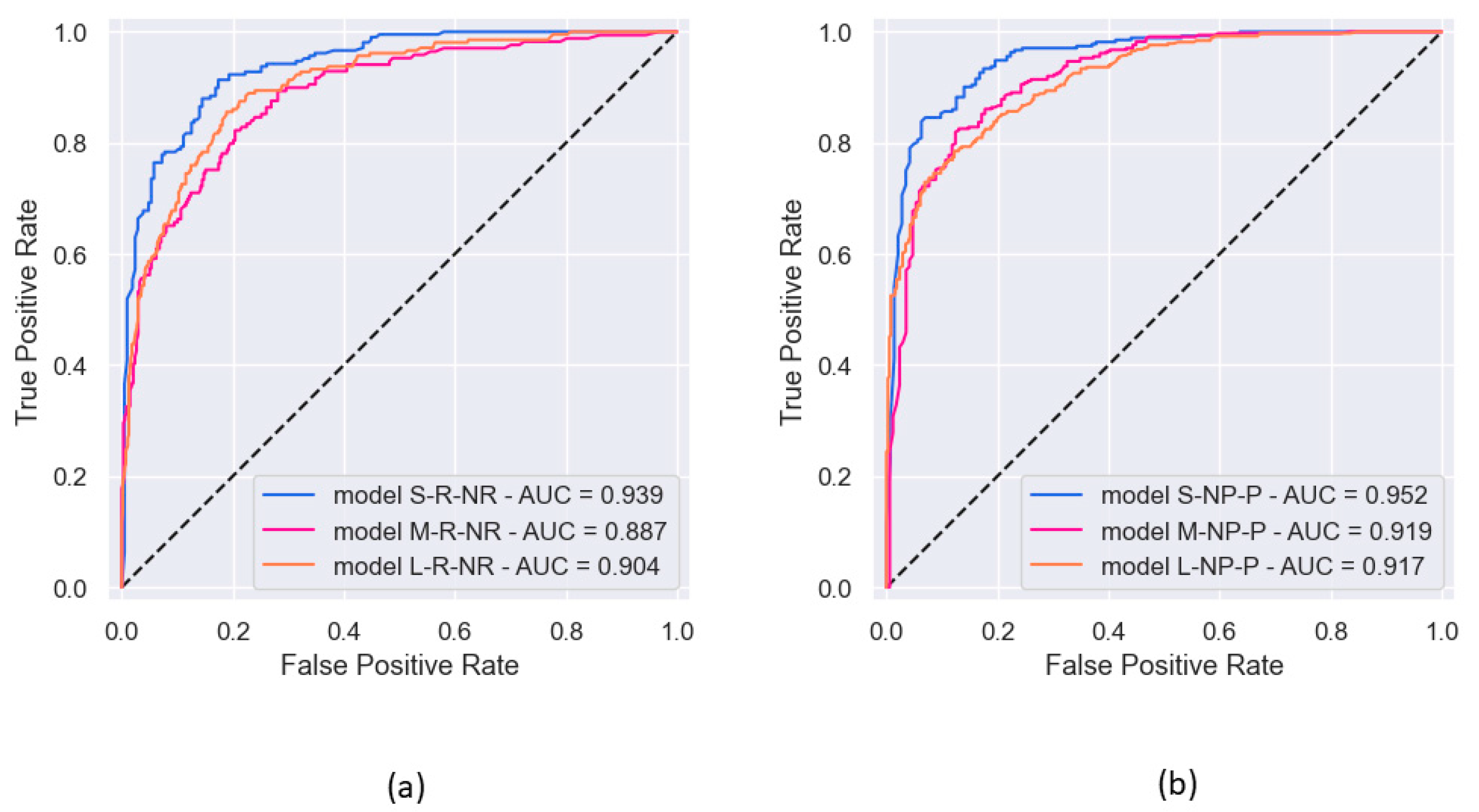
3.1.1. rEF vs. nrEF
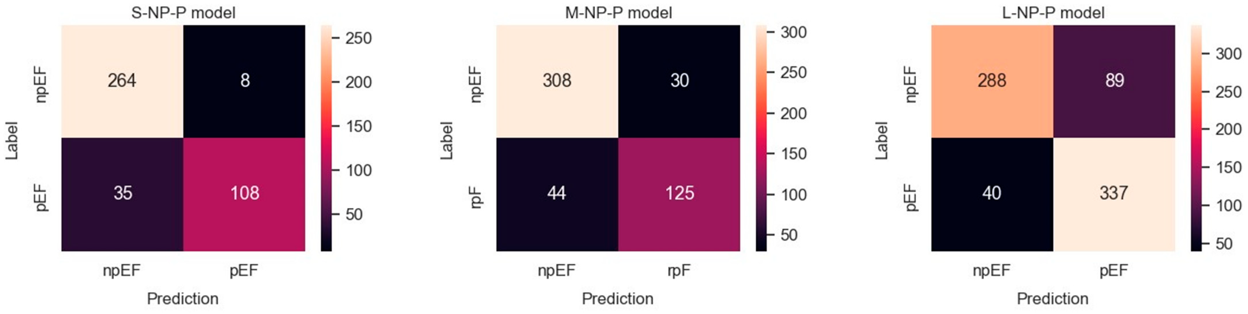
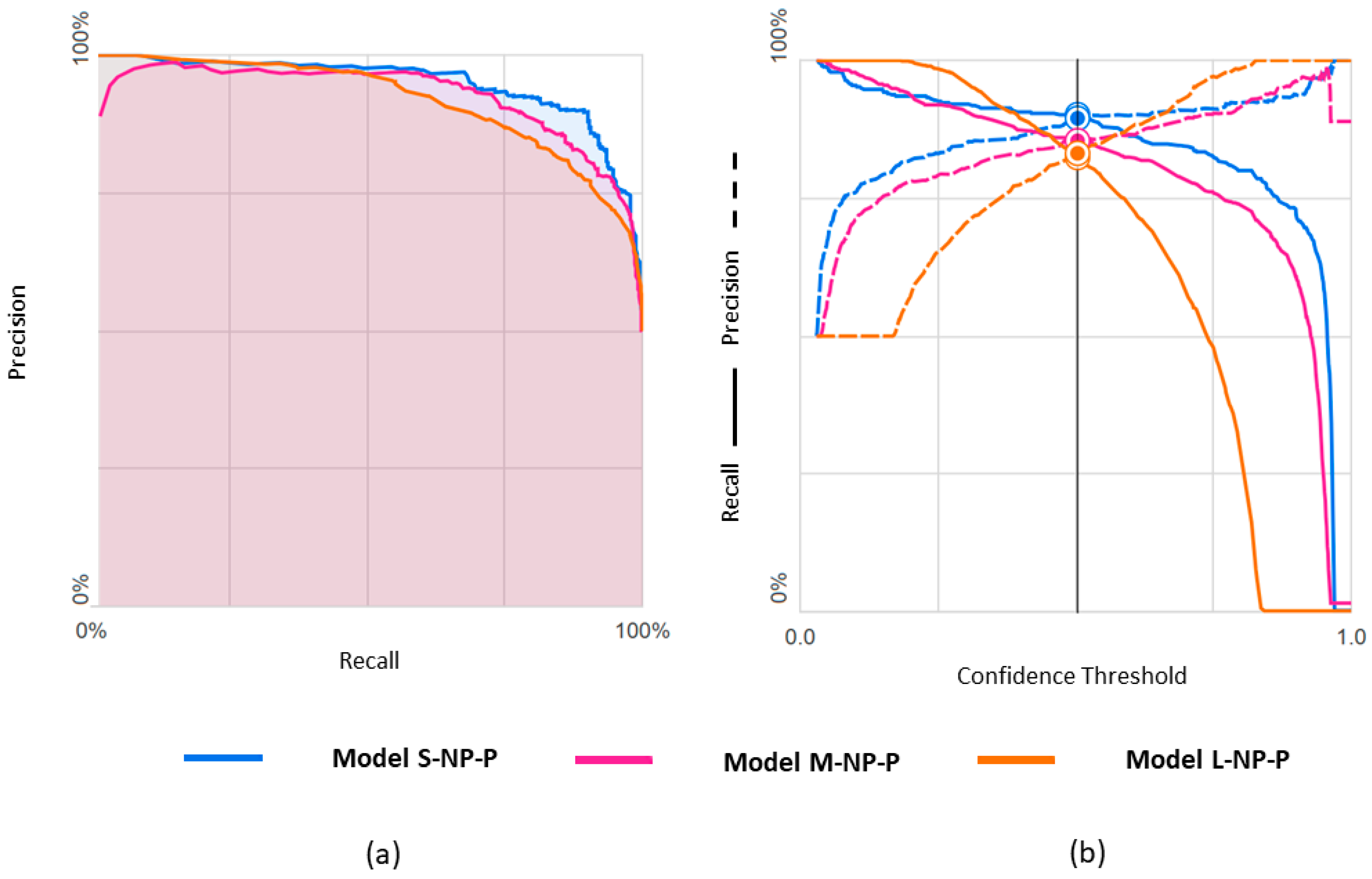
3.1.2. npEF vs. pEF
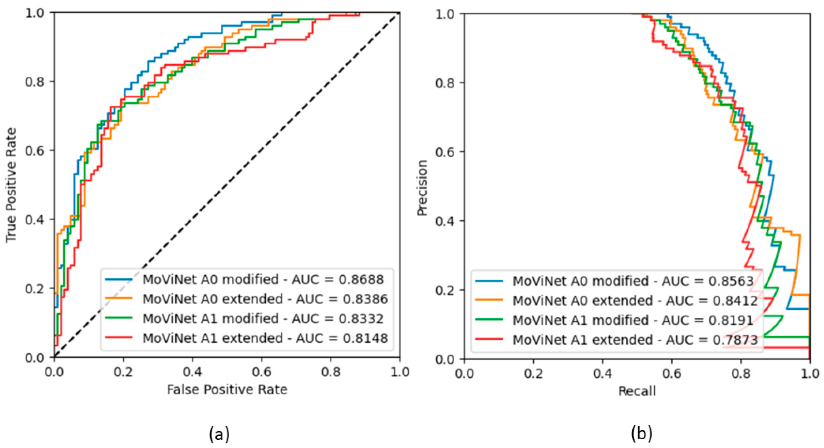
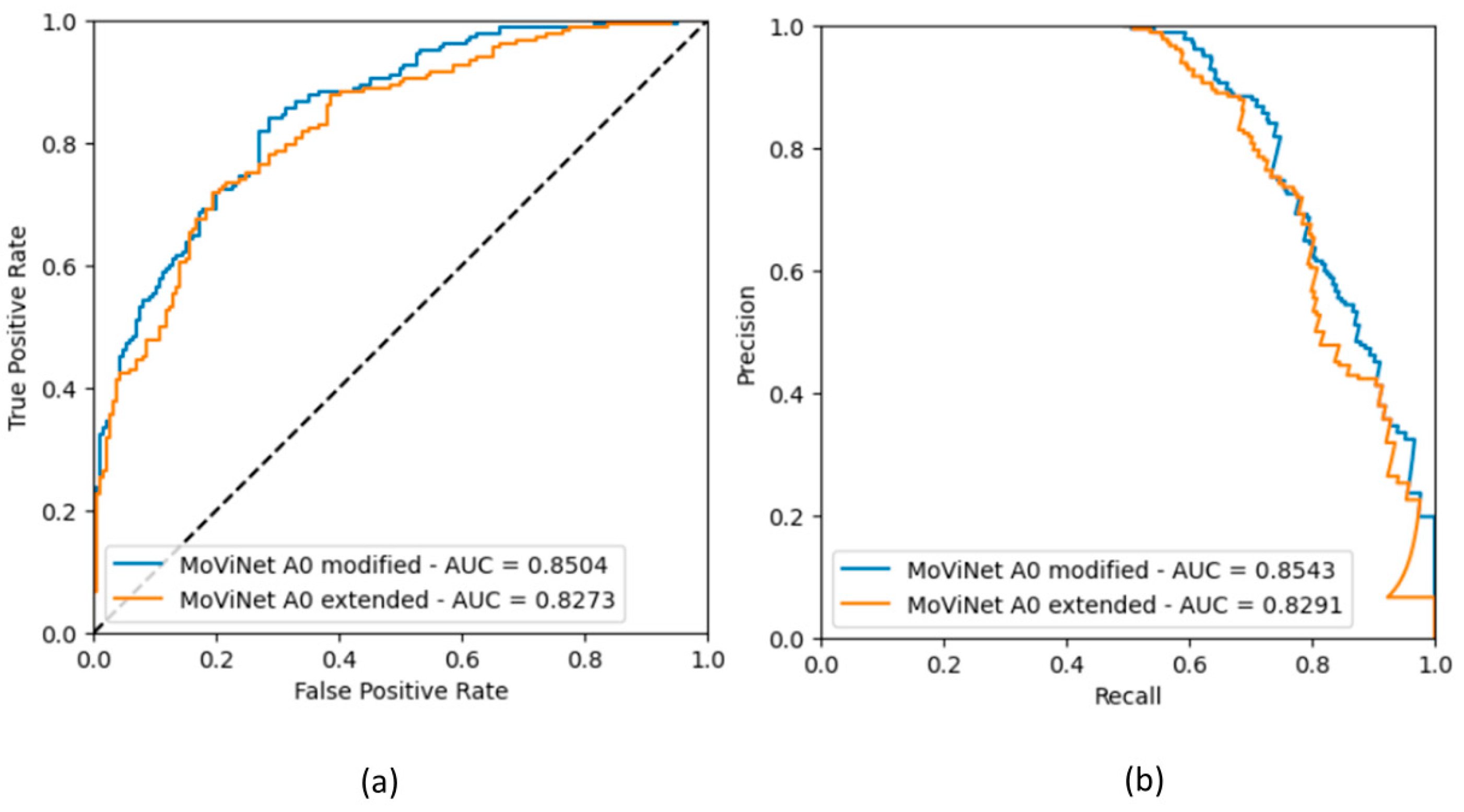
3.1.3. ROC Curves for Models with Binary Classification
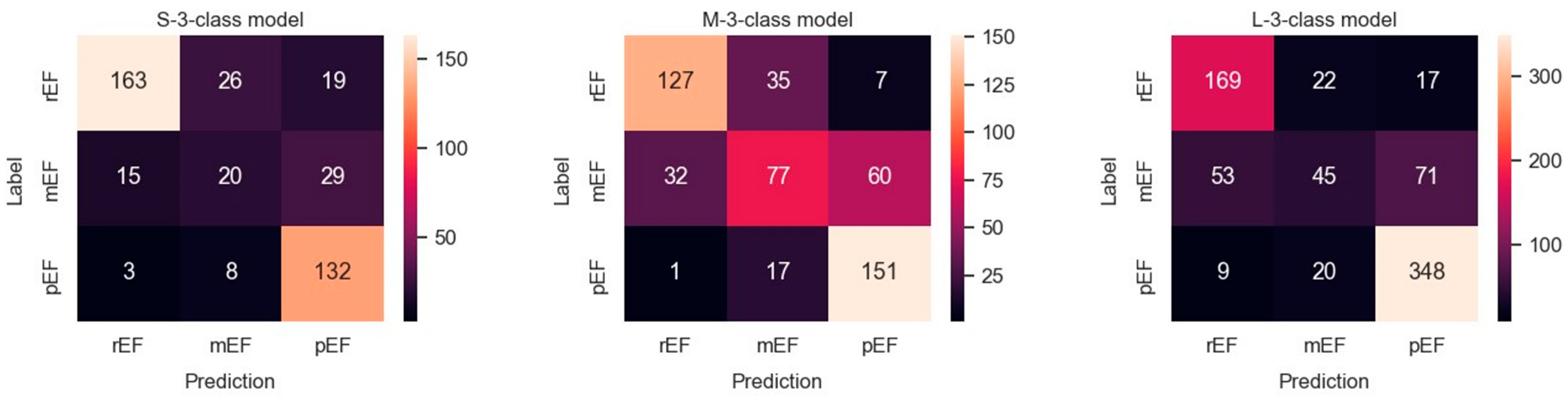
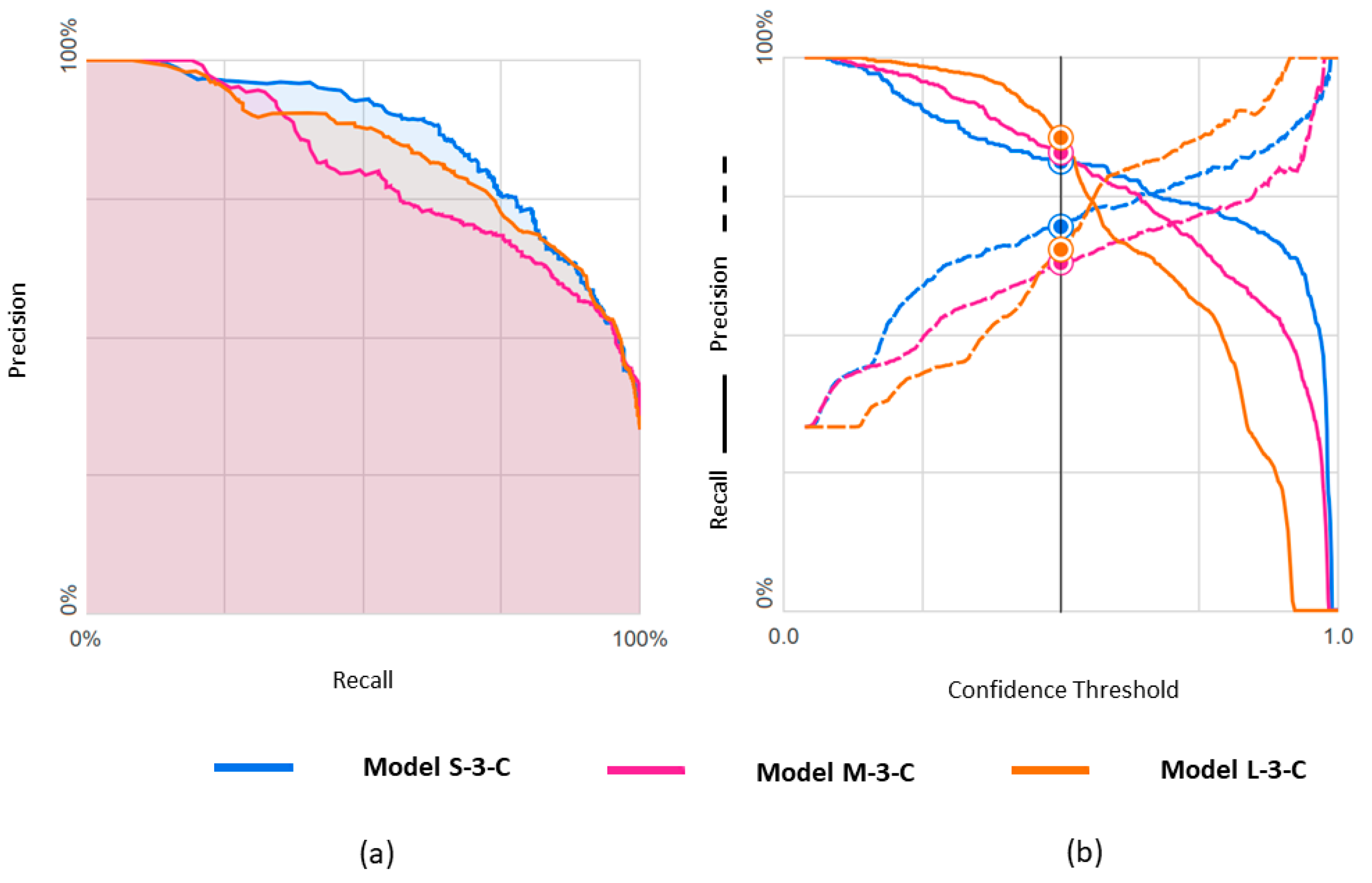
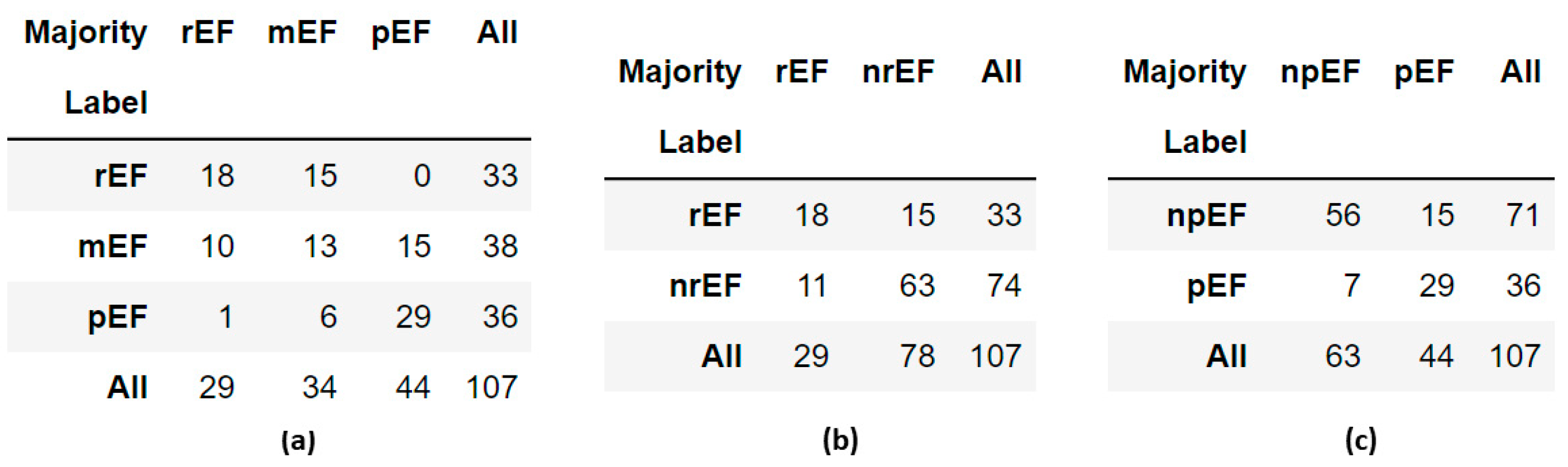
3.2. Ternary Classification
3.3. Clinician Re-Evaluation
3.4. GitHub PyTorch Implementation
4. Discussion
Author Contributions
Funding
Institutional Review Board Statement
Informed Consent Statement
Data Availability Statement
Conflicts of Interest
Appendix A

| AVI File | EF | Pred | Rater 1 | Rater 2 | Rater 3 | Rater 4 | Rater 5 | Panel |
|---|---|---|---|---|---|---|---|---|
| 0X7AB682A3B8DEC28A | 22.8 | pEF | rEF | rEF | rEF | rEF | rEF | rEF |
| 0X9756BC052F770E5 | 24.8 | nrEF | mEF | rEF | rEF | rEF | mEF Q | rEF |
| 0X73E9825196EB26F9 | 27.2 | pEF | rEF A | rEF Q A | rEF A | mEF Q A | pEF | rEF |
| 0X5216E8EAC6638EC5 | 27.7 | nrEF | rEF | rEF | rEF | rEF | rEF | rEF |
| 0X5BFC2EC0D445EA65 | 28.1 | nrEF | rEF | mEF | rEF Q A | rEF A | pEF Q | rEF |
| 0X2FAFDA5737784951 | 28.4 | nrEF | rEF | rEF | rEF | rEF | rEF | rEF |
| 0X70C7E7E952C28C1 | 28.8 | nrEF | mEF | mEF | mEF | pEF | mEF Q | mEF |
| 0X2F178A2E89C73B5 | 29.2 | pEF | pEF | pEF Q | mEF Q | mEF Q | mEF Q | mEF |
| 0X2B5619B4EDE8F1B8 | 29.3 | pEF | mEF | mEF | mEF | mEF | mEF | mEF |
| 0X260767549892A590 | 30.4 | nrEF | rEF Q A | mEF Q | rEF Q | mEF Q | rEF Q | rEF |
| 0X1FC4816F238B726E | 30.6 | pEF | rEF | rEF | rEF | rEF Q | mEF | rEF |
| 0X28C73B18FDF845BC | 30.9 | pEF | pEF A | mEF | rEF Q | rEF A | mEF Q A | mEF |
| 0X32312BC4DF1CD8A3 | 31.1 | nrEF | mEF | rEF | rEF | mEF | rEF | rEF |
| 0X3503A92D7637451 | 31.8 | nrEF | rEF Q A | rEF Q | rEF | rEF | rEF Q | rEF |
| 0X2007E059C9C83B68 | 32.6 | pEF | pEF Q | pEF Q | rEF | mEF Q | mEF | mEF |
| 0X10AD385C206C85C | 32.8 | pEF | rEF Q | mEF Q | rEF | mEF Q | mEF Q | mEF |
| 0X7329DF92A352EC62 | 33.2 | nrEF | pEF | mEF | mEF | rEF | rEF | mEF |
| 0X4A49AE73D48ED549 | 34.9 | nrEF | rEF Q | mEF Q | mEF | rEF Q | mEF Q A | mEF |
| 0X302995669B66A122 | 34.9 | nrEF | pEF Q | mEF Q | rEF Q | rEF Q | rEF | rEF |
| 0X7EEA66DBE251854B | 35.2 | nrEF | rEF A | rEF A | rEF A | mEF A | rEF | rEF |
| 0X575A1E4C8C441849 | 36.1 | nrEF | rEF | mEF Q | mEF Q | rEF Q | rEF | rEF |
| 0X560AC3ED5C9AA949 | 36.3 | pEF | rEF | rEF | rEF Q | rEF | rEF | rEF |
| 0X5C0BCAA2FB4FF1B4 | 37.4 | pEF | rEF A | mEF A | mEF Q A | mEF Q | mEF Q A | mEF |
| 0X6050E603BC35F0D | 37.7 | nrEF | rEF | rEF Q A | rEF | pEF | pEF Q A | rEF |
| 0X3285FE374F563092 | 37.8 | nrEF | mEF | mEF | mEF | mEF | rEF | mEF |
| 0X30AFF793AC29BD2B | 37.9 | nrEF | rEF | rEF | rEF | rEF | mEF | rEF |
| 0X5C7B3A4A12245C5E | 38.0 | nrEF | pEF Q | mEF Q | mEF Q | mEF Q | rEF Q | mEF |
| 0X5D78417E9211CC18 | 38.1 | nrEF | mEF Q | mEF Q | rEF Q | mEF | mEF Q A | mEF |
| 0X5042C6AB36212224 | 38.4 | nrEF | rEF | mEF | rEF Q | mEF | mEF Q | mEF |
| 0X4D17A70DB464D7EB | 39.2 | pEF | mEF A | mEF Q A | rEF | rEF | mEF | mEF |
| 0X5A887EDA76C326E9 | 39.2 | nrEF | rEF Q A | rEF | rEF | rEF | rEF | rEF |
| 0X7BA9FD251A48D45B | 39.3 | nrEF | rEF | rEF | rEF | rEF | rEF | rEF |
| 0X31E539C27D120BDE | 39.9 | nrEF | mEF | mEF | mEF Q | rEF | mEF Q | mEF |
| 0X11C89001BEF939E2 | 40.4 | pEF | rEF Q | rEF | rEF | rEF | rEF | rEF |
| 0X44F9A80B05DFC224 | 41.2 | rEF | mEF QA | pEF | rEF Q | rEF Q | pEF Q | mEF |
| 0X775319C257A48042 | 41.4 | pEF | mEF Q | mEF Q | rEF Q | rEF Q | rEF | rEF |
| 0XBD39E52A48060D2 | 42.1 | pEF | rEF | mEF | rEF | rEF | rEF | rEF |
| 0X3C63C23E5B0823D | 43.2 | pEF | rEF Q | mEF Q | rEF Q | rEF Q | rEF | rEF |
| 0X38638F441D35402 | 43.3 | rEF | pEF | mEF | mEF | rEF | rEF | mEF |
| 0X4D383DD98BD6CD12 | 43.4 | pEF | mEF | mEF | rEF | rEF | rEF | rEF |
| 0X4704159CFC29D4C3 | 43.9 | pEF | rEF A | mEF A | rEF | rEF A | mEF Q A | rEF |
| 0X2C871D22AD5EAD1A | 44.3 | rEF | pEF | mEF | mEF | pEF Q | rEF | mEF |
| 0X69B8DBAA13F1442B | 44.6 | rEF | mEF | mEF Q | rEF | mEF Q | pEF | mEF |
| 0X1337E8945A141439 | 44.7 | pEF | mEF | mEF | rEF | rEF | rEF | rEF |
| 0X13F7CAB4C719ACA3 | 45.0 | rEF | pEF | pEF | pEF | mEF | pEF | pEF |
| 0X114B58E6B34E55F1 | 45.1 | rEF | pEF | pEF Q | pEF Q | rEF Q | mEF Q | pEF |
| 0X71FE0206D64EDD39 | 45.3 | rEF | pEF | pEF Q | pEF | pEF Q | pEF | pEF |
| 0X7540B06840A33DBF | 45.4 | rEF | pEF | pEF A | pEF | pEF | mEF | pEF |
| 0X75BA1623CCCF0652 | 45.4 | pEF | mEF | mEF | rEF Q | rEF Q | rEF Q | rEF |
| 0X1C1A328EA29B6CC3 | 45.6 | rEF | pEF Q | pEF | mEF Q | pEF Q | pEF | pEF |
| 0X1F30E6AC3FE50EE3 | 46.0 | rEF | pEF Q | pEF Q | rEF Q | mEF Q | mEF Q | mEF |
| 0X6CA712DE9D936CB3 | 46.4 | rEF | pEF A | pEF A | pEF | pEF Q | pEF | pEF |
| 0XD537CD5A04B8C43 | 46.7 | rEF | pEF | pEF | pEF Q | mEF | mEF | pEF |
| 0X25D970C75A57B3F2 | 46.7 | rEF | pEF | pEF Q | pEF Q | pEF Q | pEF | pEF |
| 0X3077040EC90D916D | 46.8 | rEF | mEF | mEF | mEF Q | mEF | mEF Q | mEF |
| 0X40551ED55932933D | 46.9 | rEF | pEF | mEF Q | mEF Q | mEF Q | mEF | mEF |
| 0X15E8BE2AE8C05C88 | 46.9 | rEF | pEF | pEF | pEF | rEF Q | pEF | pEF |
| 0X6B0A6A101C2DA474 | 47.0 | rEF | pEF | pEF | mEF | mEF | mEF | mEF |
| 0X57A074E488CFB7AC | 47.2 | rEF | pEF Q | pEF Q | rEF | pEF | pEF | pEF |
| 0X3902FE711F8B581B | 48.0 | rEF | pEF | pEF | mEF | pEF | mEF Q | pEF |
| 0X35607DFD91E00F2B | 48.0 | rEF | rEF A | mEF | mEF | mEF | rEF | mEF |
| 0X65ACA3F8B770AAD7 | 48.1 | rEF | pEF | pEF | rEF Q | mEF Q | pEF Q A | pEF |
| 0X2AFCAC3003694C4D | 48.1 | pEF | mEF Q | rEF Q | rEF Q | mEF Q | rEF Q | rEF |
| 0X6A11E31F14ADFDEE | 48.3 | rEF | pEF | mEF | rEF Q | mEF | mEF | mEF |
| 0X63EFA5F7FFFB0014 | 48.4 | rEF | mEF | mEF | pEF | mEF | mEF | mEF |
| 0X5440A5C9A8CACA49 | 48.9 | rEF | pEF QA | pEF Q | pEF Q A | pEF Q A | pEF Q | pEF |
| 0X1B4F427BC662B727 | 48.9 | pEF | pEF Q | mEF | rEF Q | rEF Q | rEF | rEF |
| 0X7923B6B4614AF456 | 49.1 | rEF | rEF | mEF | mEF Q | mEF Q | mEF Q | mEF |
| 0X73CBCADA2191104C | 49.5 | rEF pEF | pEF | pEF | mEF Q | rEF Q | pEF | pEF |
| 0X26B209C0083A4AD5 | 49.8 | rEF | pEF | pEF | mEF Q | mEF Q | mEF | mEF |
| 0X3B80677CE0873E50 | 49.8 | rEF | pEF | pEF | pEF | pEF | mEF | pEF |
| 0X4191ACD0157311E5 | 50.1 | npEF | mEF | rEF | rEF Q | mEF Q | mEF Q | mEF |
| 0X16AF26F9A372EEDE | 50.5 | npEF | mEF | mEF | mEF | pEF | pEF | mEF |
| 0X2962BA442DE9E45B | 51.5 | npEF | pEF | pEF | pEF | mEF | pEF | pEF |
| 0X5AC82E1FBDF09C04 | 51.9 | npEF | pEF | pEF | rEF | mEF Q | mEF | mEF |
| 0X7871A13A25E72847 | 52.5 | npEF | pEF | pEF | mEF Q | mEF Q | mEF Q | mEF |
| 0X40253981E97848E5 | 52.9 | npEF | mEF | pEF | mEF | mEF Q | mEF | mEF |
| 0X731BBCC68C30384D | 53.4 | npEF | pEF | pEF | pEF Q | mEF | pEF | pEF |
| 0X3A3085150FD2D6E8 | 53.5 | npEF | pEF | pEF | pEF Q | rEF | pEF | pEF |
| 0X113195610E41EF2 | 54.7 | npEF | mEF Q | mEF | pEF | mEF | mEF | mEF |
| 0X5DDE9E68BB099303 | 55.1 | npEF | pEF QA | pEF | pEF Q | mEF Q | pEF Q | pEF |
| 0X210265FBDA5360AE | 55.1 | npEF | pEF | pEF | pEF | pEF | pEF | pEF |
| 0X3BFFB8615C86AE75 | 55.1 | npEF | pEF | mEF Q | rEF Q | rEF | rEF | rEF |
| 0X6E1F0B0B5831B801 | 55.7 | rEF npEF | pEF | pEF | pEF | mEF Q | pEF Q | pEF |
| 0X12807854DFA9CC01 | 56.8 | npEF | pEF | pEF | rEF Q | rEF Q | pEF | pEF |
| 0X5843363A84693349 | 57.0 | npEF | pEF Q | pEF | mEF Q | pEF Q | mEF | pEF |
| 0X77B0F03C4F1E0315 | 57.2 | npEF | pEF | pEF | pEF | pEF Q | mEF Q | pEF |
| 0X41ECEC7AAEEFD0E6 | 57.3 | rEF | pEF Q | pEF Q | pEF Q | pEF Q | pEF Q | pEF |
| 0X6AB214EB6B92DC02 | 57.3 | npEF | pEF | pEF | pEF | mEF | pEF | pEF |
| 0X2489A40319D6990E | 57.8 | rEF npEF | pEF Q | pEF | pEF | pEF | pEF | pEF |
| 0X2841EE2AE1958F10 | 58.2 | npEF | pEF | pEF | pEF | pEF | pEF | pEF |
| 0X445575CFEECB0986 | 58.7 | npEF | pEF | pEF | pEF | mEF Q | pEF | pEF |
| 0X166B717BBC2ECADA | 59.0 | npEF | pEF Q | pEF | pEF Q | pEF | pEF | pEF |
| 0X7BF746EB936C65BE | 59.1 | npEF | pEF Q A | pEF Q A | pEF Q | pEF A | pEF | pEF |
| 0X7A77DF8AACD6E023 | 59.2 | npEF | pEF | pEF | pEF | pEF Q | pEF | pEF |
| 0X8E2FCF5187C4872 | 61.1 | npEF | pEF | pEF | pEF | pEF | pEF | pEF |
| 0X1039B49145DF4F25 | 62.4 | rEF npEF | pEF | pEF | pEF | mEF Q | pEF | pEF |
| 0X5FBBC76F7AD9FB4D | 62.6 | npEF | pEF A | pEF A | pEF | pEF A | mEF Q A | pEF |
| 0X2ECE3ECC0BF62256 | 63.1 | npEF | pEF Q | pEF Q | mEF Q | pEF | pEF | pEF |
| 0X6A672DABBE9F8660 | 63.3 | npEF | pEF | pEF Q | pEF Q | pEF | pEF | pEF |
| 0X343CEAA877051407 | 63.5 | npEF | pEF | pEF | pEF | pEF Q | pEF | pEF |
| 0X73F6DA33A9F3A272 | 64.1 | npEF | pEF | pEF | pEF Q | pEF | pEF | pEF |
| 0X127D3AEEA73EDE76 | 64.7 | npEF | pEF | pEF | pEF | pEF | pEF | pEF |
| 0X5B9C0EEB93E0BE10 | 65.3 | npEF | pEF | pEF | pEF | pEF | pEF | pEF |
| 0X3E56DED8582F762B | 65.7 | npEF | pEF | pEF | pEF | pEF Q | pEF | pEF |
| 0X17828CD670289D36 | 66.9 | npEF | pEF Q | pEF Q | pEF | pEF | pEF | pEF |
| 0X4D2FF488DD4EC6BD | 70.0 | npEF | rEF | pEF Q | pEF Q | pEF Q | pEF Q | pEF |
Appendix B
Appendix B.1. Dataset and Data Curation
| Dataset | Support (Train) | Support (Validation) | Support (Test) |
|---|---|---|---|
| 1641 videos balanced for rEF vs. nrEF | 619 621 | 104 96 | 98 103 |
| 3040 videos balanced for npEF vs. pEF | 1148 1152 | 192 188 | 177 183 |
Appendix B.2. Training


Appendix B.3. Metrics
| Metrics | MoViNet A0 (Modified) rEF vs. nrEF | MoViNet A0 (Extended) rEF vs. nrEF | MoViNet A1 (Modified) rEF vs. nrEF | MoViNet A1 (Extended) rEF vs. nrEF | MoViNet A0 (Modified) npEF vs. pEF | MoViNet A0 (Extended) npEF vs. pEF |
|---|---|---|---|---|---|---|
| All labels: | ||||||
| Accuracy | 0.776 | 0.756 | 0.761 | 0.771 | 0.750 | 0.728 |
| Balanced accuracy | 0.777 | 0.756 | 0.761 | 0.772 | 0.750 | 0.738 |
| ROC AUC | 0.869 | 0.839 | 0.833 | 0.815 | 0.850 | 0.827 |
| PRC AUC | 0.856 | 0.841 | 0.819 | 0.787 | 0.854 | 0.829 |
| Label: rEF | ||||||
| Precision | 0.785 | 0.758 | 0.745 | 0.783 | 0.737 | 0.686 |
| Recall (sensitivity) | 0.745 | 0.735 | 0.776 | 0.735 | 0.769 | 0.830 |
| F1 score | 0.764 | 0.746 | 0.760 | 0.758 | 0.753 | 0.751 |
| Label: nrEF | ||||||
| Precision | 0.769 | 0.755 | 0.778 | 0.761 | 0.764 | 0.791 |
| Recall (specificity) | 0.806 | 0.777 | 0.748 | 0.806 | 0.731 | 0.629 |
| F1 score | 0.787 | 0.766 | 0.762 | 0.783 | 0.747 | 0.701 |
References
- Bui, A.L.; Horwich, T.B.; Fonarow, G.C. Epidemiology and Risk Profile of Heart Failure. Nat. Rev. Cardiol. 2010, 8, 30–41. [Google Scholar] [CrossRef] [PubMed]
- Chioncel, O.; Lainscak, M.; Seferovic, P.M.; Anker, S.D.; Crespo-Leiro, M.G.; Harjola, V.-P.; Parissis, J.; Laroche, C.; Piepoli, M.F.; Fonseca, C.; et al. Epidemiology and One-Year Outcomes in Patients with Chronic Heart Failure and Preserved, Mid-Range and Reduced Ejection Fraction: An Analysis of the ESC Heart Failure Long-Term Registry. Eur. J. Heart Fail. 2017, 19, 1574–1585. [Google Scholar] [CrossRef] [PubMed]
- Parikh, K.S.; Sharma, K.; Fiuzat, M.; Surks, H.K.; George, J.T.; Honarpour, N.; Depre, C.; Desvigne-Nickens, P.; Nkulikiyinka, R.; Lewis, G.D.; et al. Heart Failure with Preserved Ejection Fraction Expert Panel Report. JACC Heart Fail. 2018, 6, 619–632. [Google Scholar] [CrossRef] [PubMed]
- Pieske, B.; Tschöpe, C.; de Boer, R.A.; Fraser, A.G.; Anker, S.D.; Donal, E.; Edelmann, F.; Fu, M.; Guazzi, M.; Lam, C.S.P.; et al. How to Diagnose Heart Failure with Preserved Ejection Fraction: The HFA–PEFF Diagnostic Algorithm: A Consensus Recommendation from the Heart Failure Association (HFA) of the European Society of Cardiology (ESC). Eur. Heart J. 2019, 40, 3297–3317. [Google Scholar] [CrossRef] [PubMed]
- Lam, C.S.P.; Solomon, S.D. The Middle Child in Heart Failure: Heart Failure with Mid-Range Ejection Fraction (40–50%). Eur. J. Heart Fail. 2014, 16, 1049–1055. [Google Scholar] [CrossRef]
- Savarese, G.; Stolfo, D.; Sinagra, G.; Lund, L.H. Heart Failure with Mid-Range or Mildly Reduced Ejection Fraction. Nat. Rev. Cardiol. 2021, 19, 100–116. [Google Scholar] [CrossRef] [PubMed]
- Zhang, Z.; Zhu, Y.; Liu, M.; Zhang, Z.; Zhao, Y.; Yang, X.; Xie, M.; Zhang, L. Artificial Intelligence-Enhanced Echocardiography for Systolic Function Assessment. J. Clin. Med. 2022, 11, 2893. [Google Scholar] [CrossRef] [PubMed]
- EchoNet Dynamic. echonet.github.io. Available online: https://echonet.github.io/dynamic (accessed on 11 October 2023).
- Leclerc, S.; Smistad, E.; Pedrosa, J.; Ostvik, A.; Cervenansky, F.; Espinosa, F.; Espeland, T.; Berg, E.A.R.; Jodoin, P.-M.; Grenier, T.; et al. Deep Learning for Segmentation Using an Open Large-Scale Dataset in 2D Echocardiography. IEEE Trans. Med. Imaging 2019, 38, 2198–2210. [Google Scholar] [CrossRef] [PubMed]
- Ouyang, D.; He, B.; Ghorbani, A.; Yuan, N.; Ebinger, J.; Langlotz, C.P.; Heidenreich, P.A.; Harrington, R.A.; Liang, D.H.; Ashley, E.A.; et al. Video-Based AI for Beat-To-Beat Assessment of Cardiac Function. Nature 2020, 580, 252–256. [Google Scholar] [CrossRef]
- Liu, X.; Fan, Y.; Li, S.; Chen, M.; Li, M.; Hau, W.K.; Zhang, H.; Xu, L.; Lee, A.P.-W. Deep Learning-Based Automated Left Ventricular Ejection Fraction Assessment Using 2-D Echocardiography. Am. J. Physiol.-Heart Circ. Physiol. 2021, 321, H390–H399. [Google Scholar] [CrossRef]
- Belfilali, H.; Bousefsaf, F.; Messadi, M. Left ventricle analysis in echocardiographic images using transfer learning. Phys. Eng. Sci. Med. 2022, 45, 1123–1138. [Google Scholar] [CrossRef] [PubMed]
- Aubry, A.; Duong, L. Automatic Evaluation of the Ejection Fraction on Echocardiography Images. CMBES Proc. 2023, 45, 1–4. Available online: https://proceedings.cmbes.ca/index.php/proceedings/article/view/995 (accessed on 8 October 2023).
- Susan, S.; Kumar, A. The Balancing Trick: Optimized Sampling of Imbalanced Datasets—A Brief Survey of the Recent State of the Art. Eng. Rep. 2020, 3, e12298. [Google Scholar] [CrossRef]
- Singh, V.; Pencina, M.; Einstein, A.J.; Liang, J.X.; Berman, D.S.; Slomka, P. Impact of Train/Test Sample Regimen on Performance Estimate Stability of Machine Learning in Cardiovascular Imaging. Sci. Rep. 2021, 11, 14490. [Google Scholar] [CrossRef] [PubMed]
- Sveric, K.M.; Botan, R.; Dindane, Z.; Winkler, A.; Nowack, T.; Heitmann, C.; Schleußner, L.; Linke, A. Single-Site Experience with an Automated Artificial Intelligence Application for Left Ventricular Ejection Fraction Measurement in Echocardiography. Diagnostics 2023, 13, 1298. [Google Scholar] [CrossRef] [PubMed]
- Tuggener, L.; Amirian, M.; Benites, F.; von Däniken, P.; Gupta, P.; Schilling, F.-P.; Stadelmann, T. Design Patterns for Resource-Constrained Automated Deep-Learning Methods. AI 2020, 1, 510–538. [Google Scholar] [CrossRef]
- Waring, J.; Lindvall, C.; Umeton, R. Automated Machine Learning: Review of the State-of-The-Art and Opportunities for Healthcare. Artif. Intell. Med. 2020, 104, 101822. [Google Scholar] [CrossRef] [PubMed]
- Katti, J.; Agarwal, J.; Bharata, S.; Shinde, S.; Mane, S.; Biradar, V. University Admission Prediction Using Google Vertex AI. In Proceedings of the 2022 First International Conference on Artificial Intelligence Trends and Pattern Recognition (ICAITPR), Hyderabad, India, 10–12 March 2022. [Google Scholar] [CrossRef]
- Mahajan, N.; Holzwanger, E.; Brown, J.; Berzin, T.M. Deploying Automated Machine Learning for Computer Vision Projects: A Brief Introduction for Endoscopists. VideoGIE 2023, 8, 249–251. [Google Scholar] [CrossRef] [PubMed]
- Davis, J.; Goadrich, M. The Relationship between Precision-Recall and ROC Curves. minds.wisconsin.edu. Available online: http://digital.library.wisc.edu/1793/60482 (accessed on 11 October 2023).
- Liu, M.; Cheng, D.; Wang, K.; Wang, Y. Multi-Modality Cascaded Convolutional Neural Networks for Alzheimer’s Disease Diagnosis. Neuroinformatics 2018, 16, 295–308. [Google Scholar] [CrossRef]
- Yagis, E.; Citi, L.; Diciotti, S.; Marzi, C.; Atnafu, S.W.; De Herrera, A.G.S. 3D Convolutional Neural Networks for Diagnosis of Alzheimer’s Disease via Structural MRI. In Proceedings of the 2020 IEEE 33rd International Symposium on Computer-Based Medical Systems (CBMS), Rochester, MN, USA, 28–30 July 2020. [Google Scholar] [CrossRef]
- Mehmet Günhan Ertosun; Rubin, D.L. Automated Grading of Gliomas Using Deep Learning in Digital Pathology Images: A Modular Approach with Ensemble of Convolutional Neural Networks. AMIA Annu. Symp. Proc. 2015, 2015, 1899. Available online: https://www.ncbi.nlm.nih.gov/pmc/articles/pmid/26958289/ (accessed on 8 October 2023).
- Sultan, H.H.; Salem, N.M.; Al-Atabany, W. Multi-Classification of Brain Tumor Images Using Deep Neural Network. IEEE Access 2019, 7, 69215–69225. [Google Scholar] [CrossRef]
- Valverde, J.M.; Imani, V.; Abdollahzadeh, A.; De Feo, R.; Prakash, M.; Ciszek, R.; Tohka, J. Transfer Learning in Magnetic Resonance Brain Imaging: A Systematic Review. J. Imaging 2021, 7, 66. [Google Scholar] [CrossRef]
- Mukhlif, A.A.; Al-Khateeb, B.; Mohammed, M.A. An Extensive Review of State-of-The-Art Transfer Learning Techniques Used in Medical Imaging: Open Issues and Challenges. J. Intell. Syst. 2022, 31, 1085–1111. [Google Scholar] [CrossRef]
- Bressem, K.K.; Adams, L.C.; Erxleben, C.; Hamm, B.; Niehues, S.M.; Vahldiek, J.L. Comparing Different Deep Learning Architectures for Classification of Chest Radiographs. Sci. Rep. 2020, 10, 13590. [Google Scholar] [CrossRef]
- Wang, X.; Peng, Y.; Lu, L.; Lu, Z.; Bagheri, M.; Summers, R.M. ChestX-Ray8: Hospital-Scale Chest X-ray Database and Benchmarks on Weakly-Supervised Classification and Localization of Common Thorax Diseases. In Proceedings of the 2017 IEEE Conference on Computer Vision and Pattern Recognition (CVPR), Honolulu, HI, USA, 21–26 July 2017. [Google Scholar] [CrossRef]
- Matsumoto, T.; Kodera, S.; Shinohara, H.; Ieki, H.; Yamaguchi, T.; Higashikuni, Y.; Kiyosue, A.; Ito, K.; Ando, J.; Takimoto, E.; et al. Diagnosing Heart Failure from Chest X-ray Images Using Deep Learning. Int. Heart J. 2020, 61, 781–786. [Google Scholar] [CrossRef] [PubMed]
- Rajpurkar, P.; Irvin, J.; Ball, R.L.; Zhu, K.; Yang, B.; Mehta, H.; Duan, T.; Ding, D.; Bagul, A.; Langlotz, C.P.; et al. Deep Learning for Chest Radiograph Diagnosis: A Retrospective Comparison of the CheXNeXt Algorithm to Practicing Radiologists. PLoS Med. 2018, 15, e1002686. [Google Scholar] [CrossRef]
- Arun, N.; Gaw, N.; Singh, P.; Chang, K.; Aggarwal, M.; Chen, B.; Hoebel, K.; Gupta, S.; Patel, J.; Gidwani, M.; et al. Assessing the Trustworthiness of Saliency Maps for Localizing Abnormalities in Medical Imaging. Radiol. Artif. Intell. 2021, 3, e200267. [Google Scholar] [CrossRef]
- Abbas, A.; Sutter, D.; Zoufal, C.; Lucchi, A.; Figalli, A.; Woerner, S. The Power of Quantum Neural Networks. Nat. Comput. Sci. 2021, 1, 403–409. [Google Scholar] [CrossRef] [PubMed]
- Mari, A.; Bromley, T.R.; Izaac, J.; Schuld, M.; Killoran, N. Transfer Learning in Hybrid Classical-Quantum Neural Networks. Quantum 2020, 4, 340. [Google Scholar] [CrossRef]
- Subbiah, G.; Krishnakumar, S.S.; Asthana, N.; Balaji, P.; Vaiyapuri, T. Quantum Transfer Learning for Image Classification. TELKOMNIKA (Telecommun. Comput. Electron. Control) 2023, 21, 113. [Google Scholar] [CrossRef]
- Shahwar, T.; Zafar, J.; Almogren, A.; Zafar, H.; Rehman, A.U.; Shafiq, M.; Hamam, H. Automated Detection of Alzheimer’s via Hybrid Classical Quantum Neural Networks. Electronics 2022, 11, 721. [Google Scholar] [CrossRef]
- Ovalle-Magallanes, E.; Avina-Cervantes, J.G.; Cruz-Aceves, I.; Ruiz-Pinales, J. Hybrid Classical–Quantum Convolutional Neural Network for Stenosis Detection in X-ray Coronary Angiography. Expert Syst. Appl. 2022, 189, 116112. [Google Scholar] [CrossRef]
- Decoodt, P.; Liang, T.J.; Bopardikar, S.; Santhanam, H.; Eyembe, A.; Garcia-Zapirain, B.; Sierra-Sosa, D. Hybrid Classical–Quantum Transfer Learning for Cardiomegaly Detection in Chest X-rays. J. Imaging 2023, 9, 128. [Google Scholar] [CrossRef]
- Alsharabi, N.; Shahwar, T.; Rehman, A.U.; Alharbi, Y. Implementing Magnetic Resonance Imaging Brain Disorder Classification via AlexNet–Quantum Learning. Mathematics 2023, 11, 376. [Google Scholar] [CrossRef]
- kkroening/ffmpeg-python: Python Bindings for FFmpeg—With Complex Filtering Support. Available online: https://github.com/kkroening/ffmpeg-python (accessed on 3 April 2024).
- Available online: https://pytorch.org/vision/stable/models.html#video-classification (accessed on 3 April 2024).
- Available online: https://github.com/Atze00/MoViNet-pytorch (accessed on 3 April 2024).
- Kingma, D.P.; Ba, J. Adam: A Method for Stochastic Optimization. arXiv 2017, arXiv:1412.6980. [Google Scholar]


| Dataset | Label * | Support (Train) | Support (Test) |
|---|---|---|---|
| S-set: 1658 videos Balanced for rEF vs. nrEF | rEF | 621 | 208 |
| mEF | 197 | 64 | |
| pEF | 425 | 143 | |
| M-set: 2109 videos Balanced for all three classes | rEF | 534 | 169 |
| mEF | 534 | 169 | |
| pEF | 534 | 169 | |
| L-set: 3064 videos Balanced for npEF vs. pEF | rEF | 621 | 208 |
| mEF | 534 | 169 | |
| pEF | 1155 | 377 |
| Model | Dataset | Classification | Job Duration |
|---|---|---|---|
| S-R-NR | S-set | Binary: rEF vs. nrEF | 3 h 49 min |
| S-NP-P | S-set | Binary: npEF vs. pEF | 3 h 18 min |
| S-3-C | S-set | Ternary: rEF, mEF, pEF | 3 h 53 min |
| M-R-NR | M-set | Binary: rEF vs. nrEF | 6 h 9 min |
| M-NP-P | M-set | Binary: npEF vs. pEF | 5 h 9 min |
| M-3-C | M-set | Ternary: rEF, mEF, pEF | 4 h 29 min |
| L-R-NR | L-set | Binary: rEF vs. nrEF | 2 h 50 min |
| L-NP-P | L-set | Binary: npEF vs. pEF | 2 h 34 min |
| L-3-C | L-set | Ternary: rEF, mEF, pEF | 2 h 49 min |
| Classifier | Metrics | S-Set | M-Set | L-Set |
|---|---|---|---|---|
| Binary: rEF vs. nrEF | All labels: | |||
| Accuracy | 0.863 | 0.822 | 0.845 | |
| Balanced accuracy | 0.863 | 0.796 | 0.816 | |
| ROC AUC | 0.939 | 0.896 | 0.904 | |
| PRC AUC * | 0.935 | 0.904 | 0.926 | |
| Label: rEF | ||||
| Precision | 0.842 | 0.745 | 0.708 | |
| Recall (sensitivity) | 0.894 | 0.710 | 0.736 | |
| F1 score | 0.867 | 0.727 | 0.722 | |
| Label: nrEF | ||||
| Precision | 0.887 | 0.858 | 0.891 | |
| Recall (specificity) | 0.831 | 0.879 | 0.896 | |
| F1 score | 0.858 | 0.868 | 0.893 | |
| Binary: npEF vs. pEF | All labels: | |||
| Accuracy | 0.896 | 0.854 | 0.829 | |
| Balanced accuracy | 0.870 | 0.829 | 0.826 | |
| ROC AUC | 0.952 | 0.919 | 0.917 | |
| PRC AUC * | 0.948 | 0.924 | 0.918 | |
| Label: pEF | ||||
| Precision | 0.924 | 0.808 | 0.792 | |
| Recall (specificity) | 0.769 | 0.746 | 0.891 | |
| F1 score | 0.840 | 0.775 | 0.839 | |
| Label: npEF | ||||
| Precision | 0.883 | 0.875 | 0.888 | |
| Recall (sensitivity) | 0.971 | 0.911 | 0.761 | |
| F1 score | 0.925 | 0.893 | 0.817 |
| Classifier | Metrics | S-Set | M-Set | L-Set |
|---|---|---|---|---|
| Ternary: rEF, mEF, pEF | All labels: | |||
| Accuracy | 0.759 | 0.700 | 0.745 | |
| Balanced accuracy | 0.740 | 0.829 | 0.817 | |
| PRC AUC * | 0.856 | 0.795 | 0.829 | |
| Label: rEF | ||||
| Precision | 0.883 | 0.749 | 0.697 | |
| Recall | 0.837 | 0.811 | 0.851 | |
| F1 score | 0.859 | 0.778 | 0.766 | |
| Label: mEF | ||||
| Precision | 0.295 | 0.545 | 0.403 | |
| Recall | 0.438 | 0.716 | 0.651 | |
| F1 score | 0.352 | 0.619 | 0.498 | |
| Label: pEF | ||||
| Precision | 0.699 | 0.618 | 0.778 | |
| Recall | 0.944 | 0.959 | 0.950 | |
| F1 score | 0.804 | 0.752 | 0.855 |
Disclaimer/Publisher’s Note: The statements, opinions and data contained in all publications are solely those of the individual author(s) and contributor(s) and not of MDPI and/or the editor(s). MDPI and/or the editor(s) disclaim responsibility for any injury to people or property resulting from any ideas, methods, instructions or products referred to in the content. |
© 2024 by the authors. Licensee MDPI, Basel, Switzerland. This article is an open access article distributed under the terms and conditions of the Creative Commons Attribution (CC BY) license (https://creativecommons.org/licenses/by/4.0/).
Share and Cite
Decoodt, P.; Sierra-Sosa, D.; Anghel, L.; Cuminetti, G.; De Keyzer, E.; Morissens, M. Transfer Learning Video Classification of Preserved, Mid-Range, and Reduced Left Ventricular Ejection Fraction in Echocardiography. Diagnostics 2024, 14, 1439. https://doi.org/10.3390/diagnostics14131439
Decoodt P, Sierra-Sosa D, Anghel L, Cuminetti G, De Keyzer E, Morissens M. Transfer Learning Video Classification of Preserved, Mid-Range, and Reduced Left Ventricular Ejection Fraction in Echocardiography. Diagnostics. 2024; 14(13):1439. https://doi.org/10.3390/diagnostics14131439
Chicago/Turabian StyleDecoodt, Pierre, Daniel Sierra-Sosa, Laura Anghel, Giovanni Cuminetti, Eva De Keyzer, and Marielle Morissens. 2024. "Transfer Learning Video Classification of Preserved, Mid-Range, and Reduced Left Ventricular Ejection Fraction in Echocardiography" Diagnostics 14, no. 13: 1439. https://doi.org/10.3390/diagnostics14131439
APA StyleDecoodt, P., Sierra-Sosa, D., Anghel, L., Cuminetti, G., De Keyzer, E., & Morissens, M. (2024). Transfer Learning Video Classification of Preserved, Mid-Range, and Reduced Left Ventricular Ejection Fraction in Echocardiography. Diagnostics, 14(13), 1439. https://doi.org/10.3390/diagnostics14131439