
A Deep Learning Framework with an Intermediate Layer Using the Swarm Intelligence Optimizer for Diagnosing Oral Squamous Cell Carcinoma

 , , , and
Abstract
:1. Introduction
- The proposal of a novel deep learning framework that includes a swarm intelligence-based optimization algorithm as an intermediate layer in the deep learning model.
- The development of MGTO with appropriate modifications that enhance classification accuracy.
- A comparative analysis of popular deep learning models with and without the proposed intermediate layer in terms of various classification metrics and training times.
2. Related Work
3. Background
3.1. CNN
3.2. InceptionV2
3.3. MobileNetV3
3.4. EfficientNetB3
3.5. Gorilla Troops Optimization
3.6. Particle Swarm Optimization
3.7. Elephant Herding Optimization
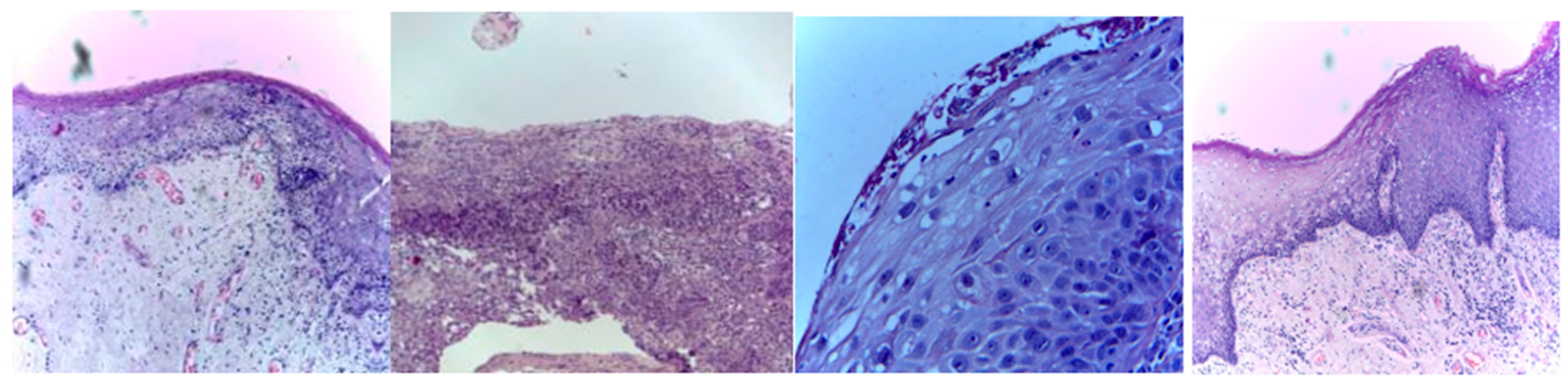
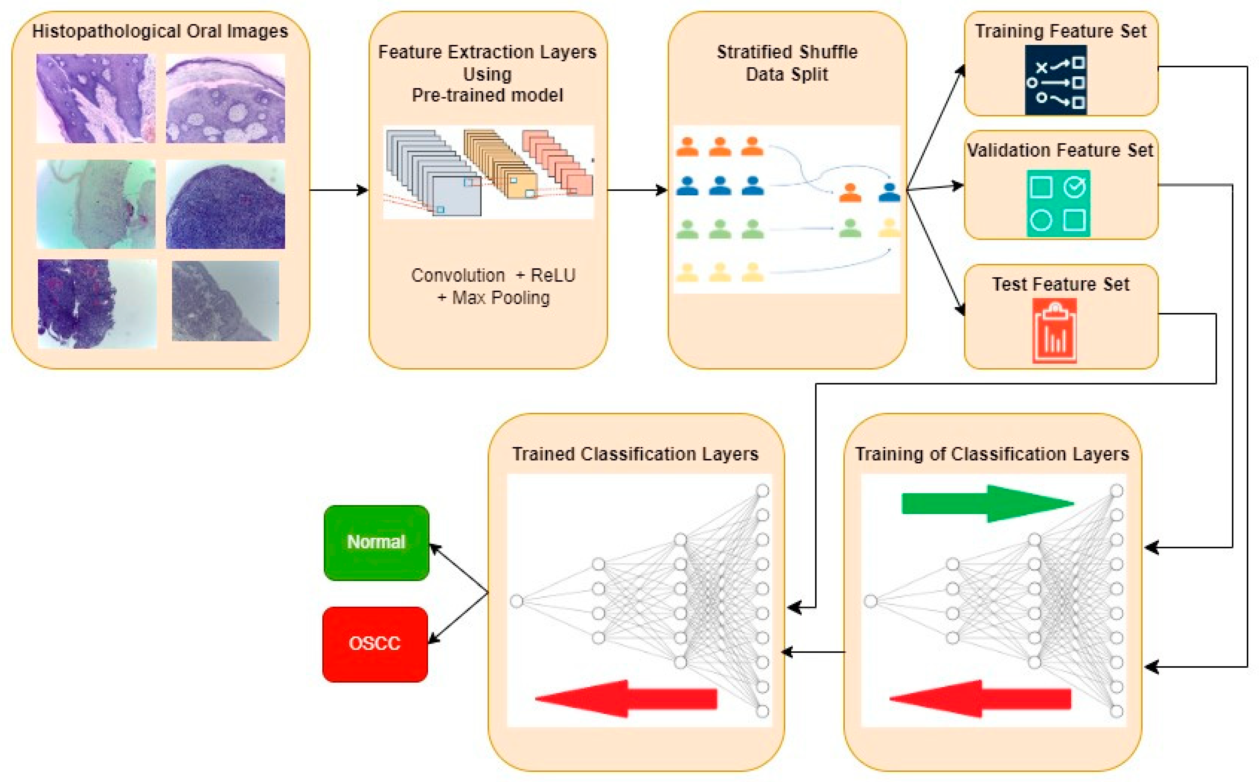
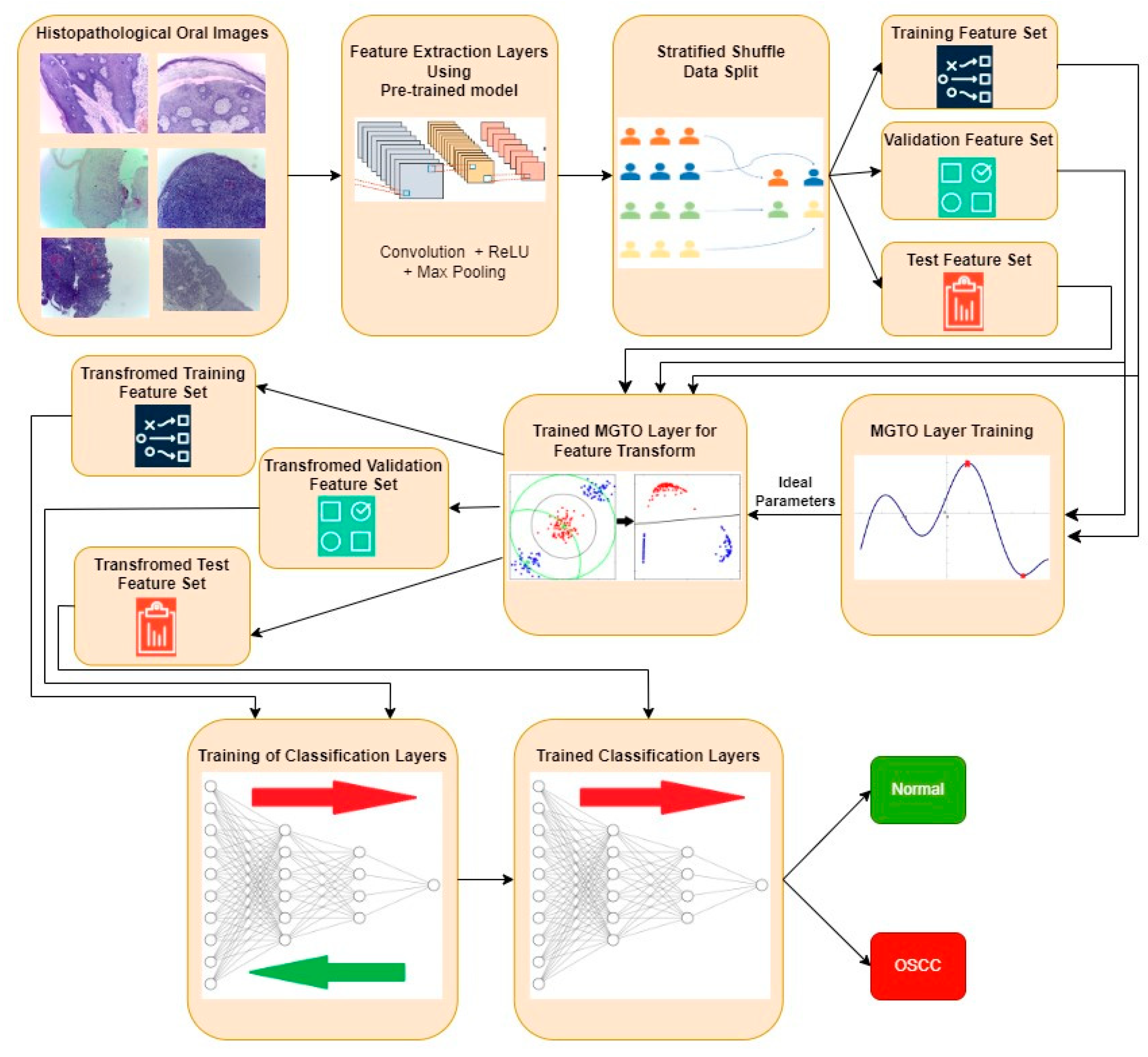
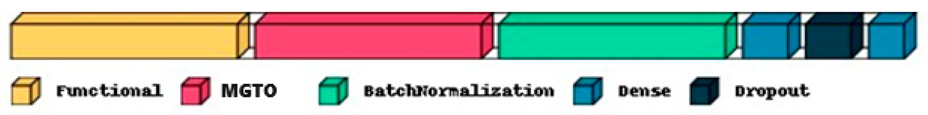
4. Materials and Methods
5. Implementation of the Proposed MGTO
| Algorithm 1: Algorithm to implement the proposed MGTO as an intermediate layer in deep learning models for feature transformation of a test feature set. |
| Step 1: Extract features using pre-trained transfer learning models for each oral histopathological image. Step 2: Consider the number of features as the size of the population in MGTO. Initialize the position of gorillas with extracted features. Step 3: Initialize parameters of MGTO: , , = 0.3, and = 0.7. Step 4: Compute the fitness value of each gorilla using Equation (25). Step 5: Update the position of each gorilla using Equation (21). Step 6: Identify the silverback gorilla, i.e., the gorilla with the highest fitness. Step 7: Update the position of each gorilla using Equation (22) if . Otherwise, use Equation (23). Step 8: Repeat steps 4 to 7 until the maximum number of iterations is reached. If the maximum number of iterations are completed, then go to step 9. Step 9: Consider the final position of the gorillas as the output of the feature transform and give them as input to the classification layer. |
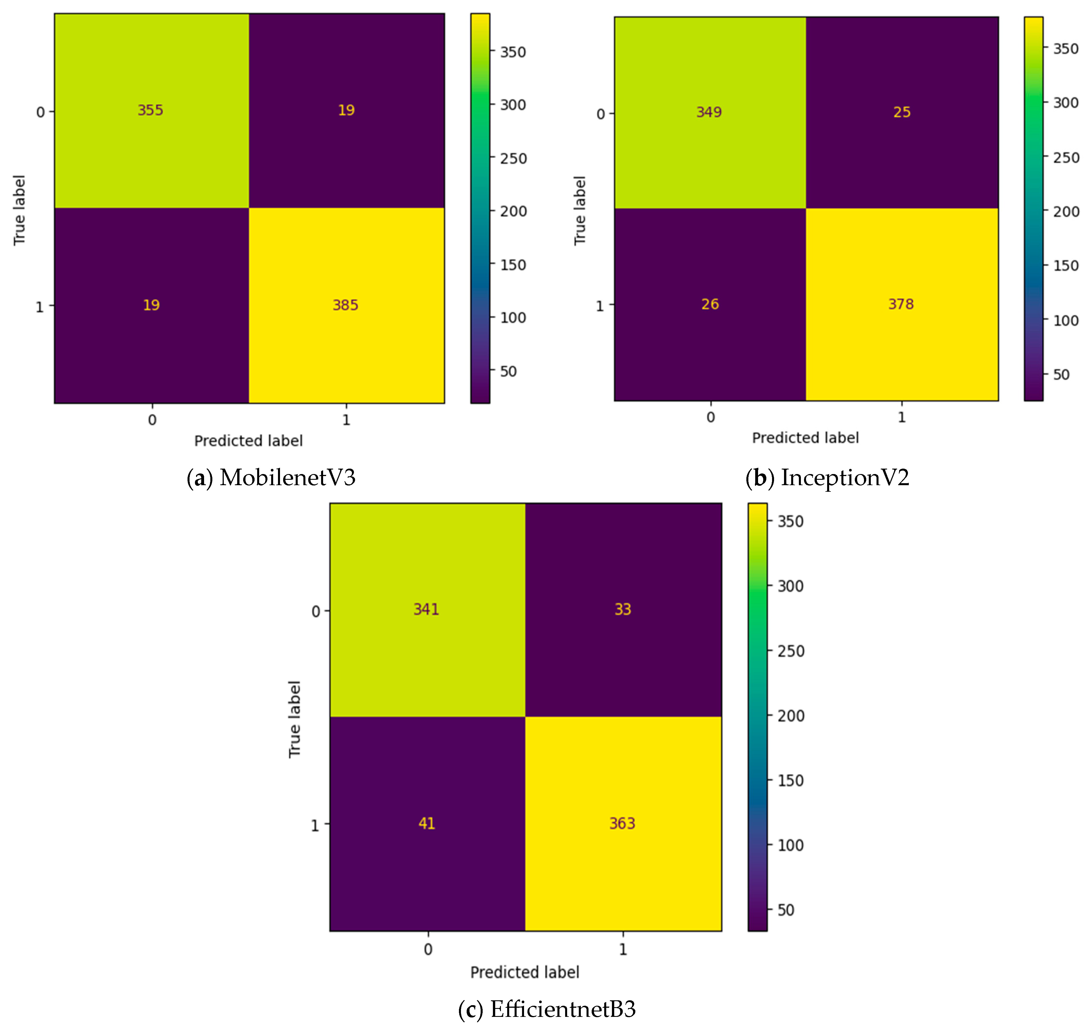
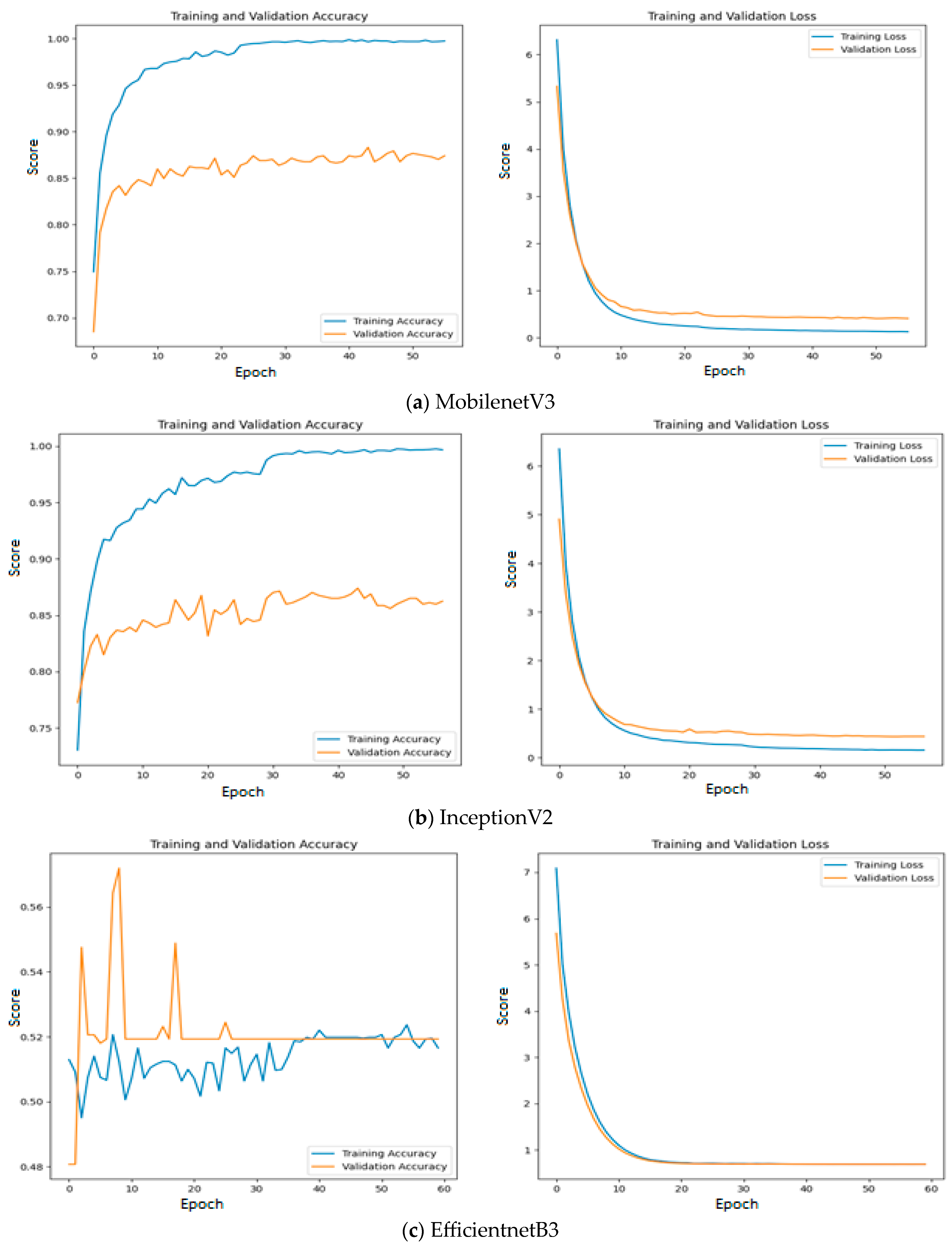
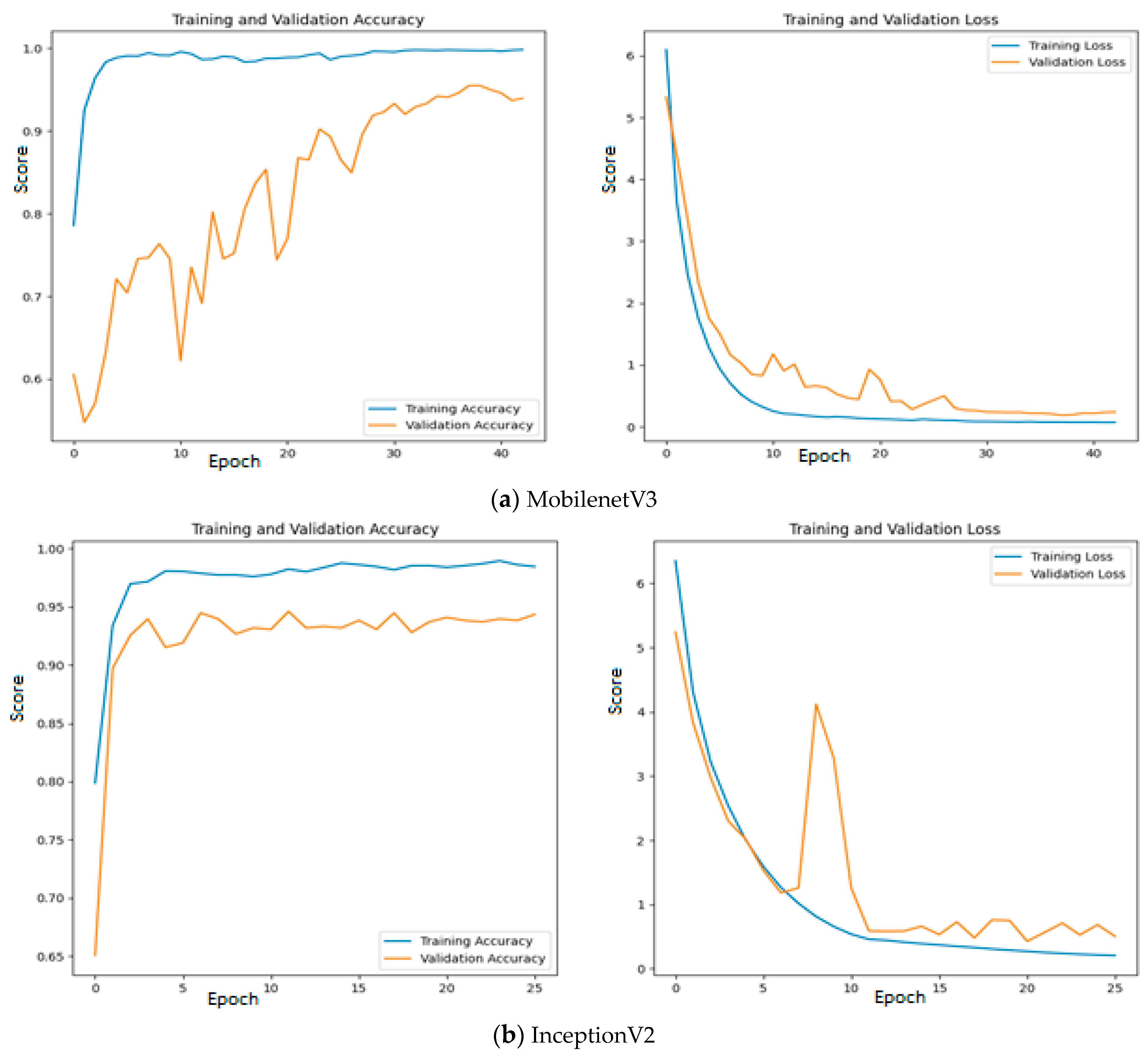
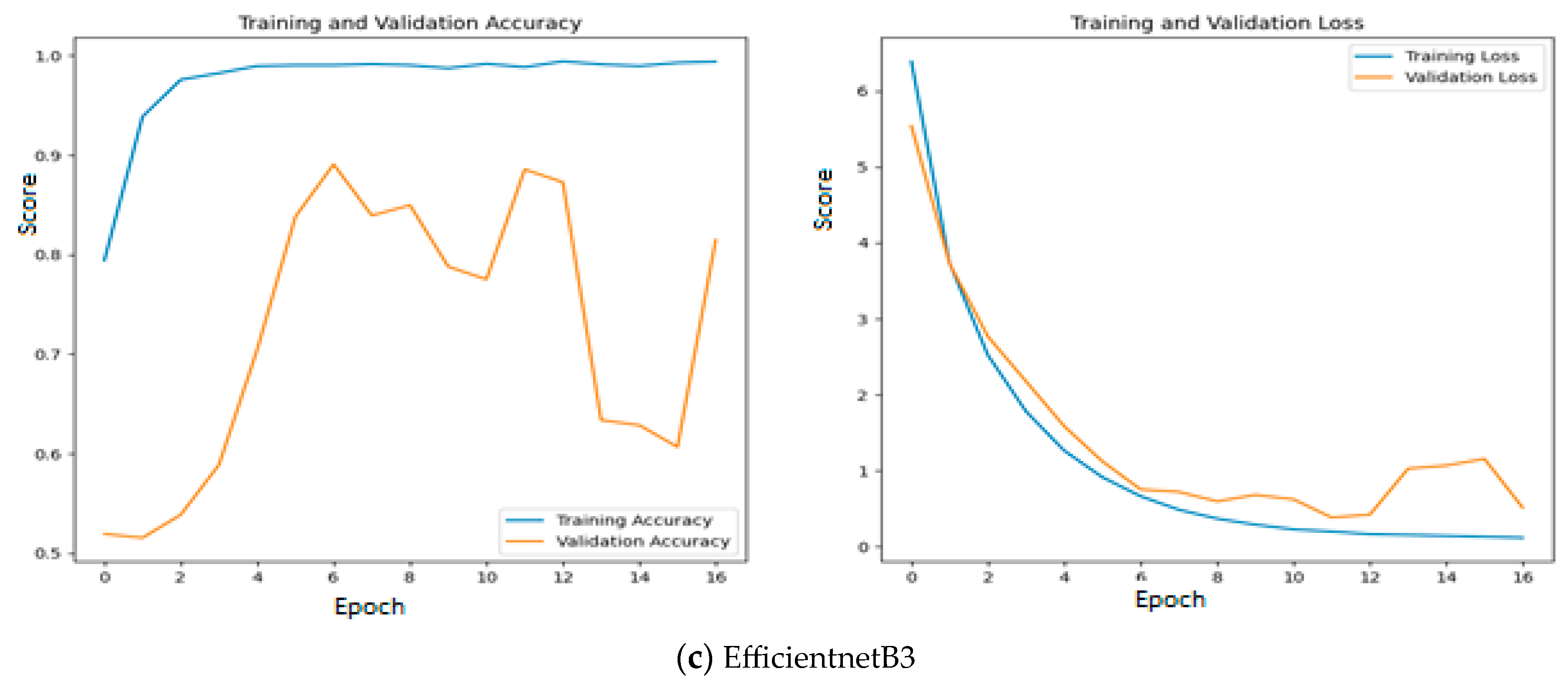
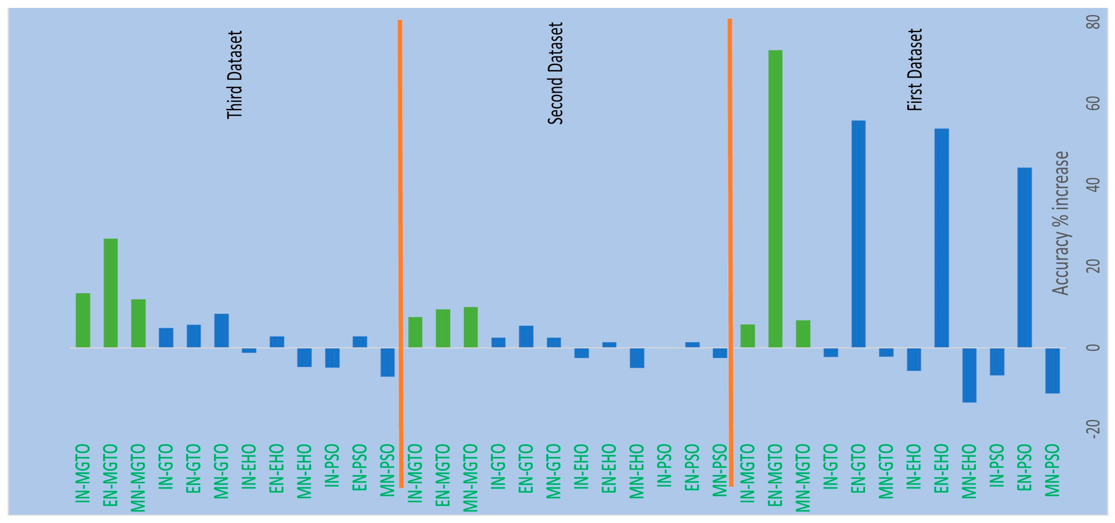
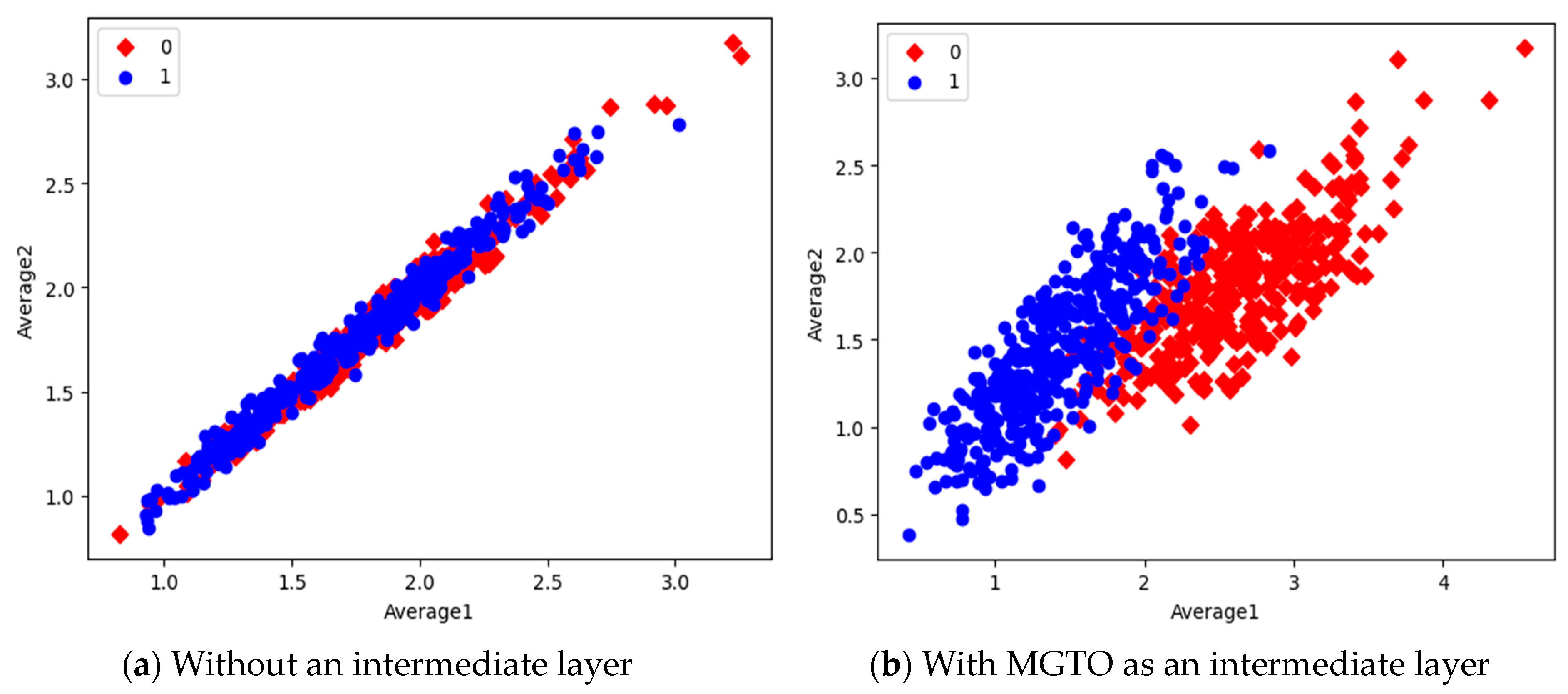
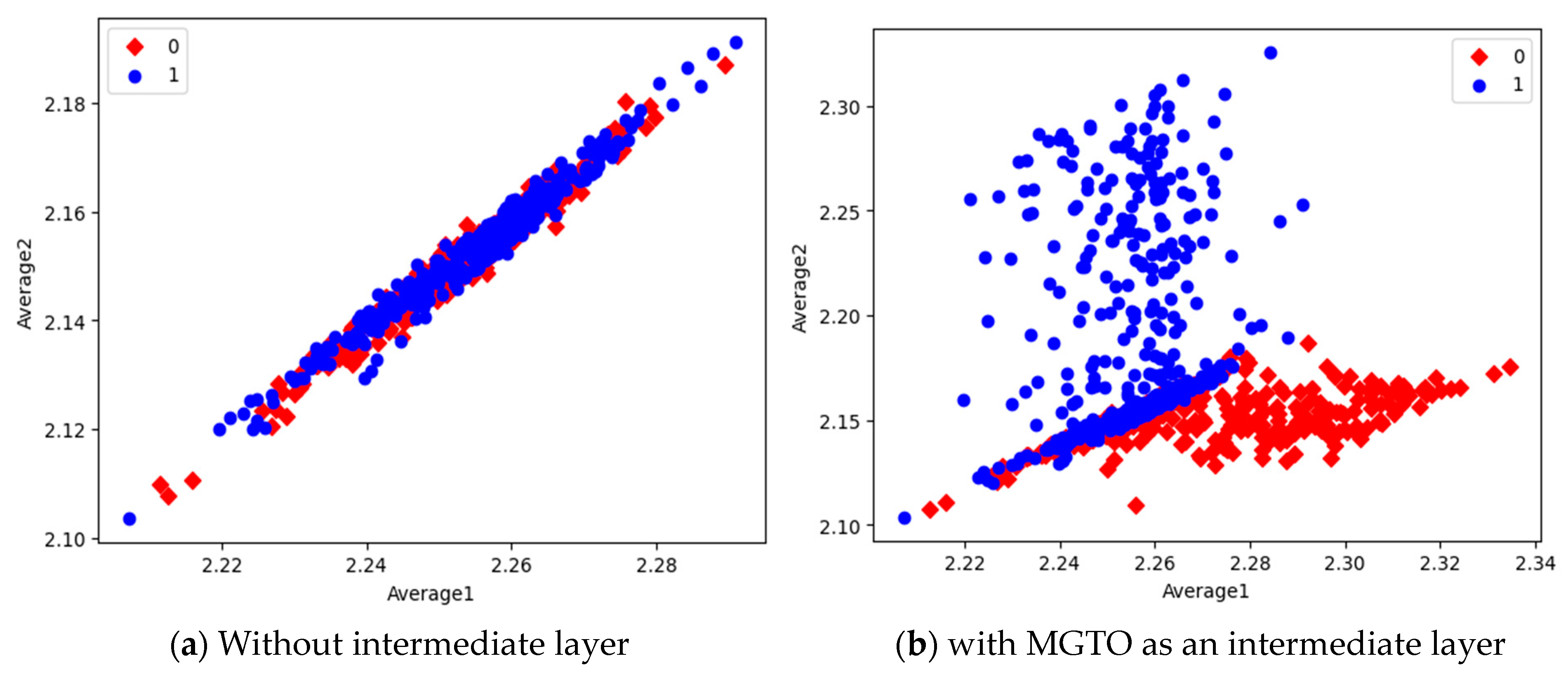
6. Results and Discussion
7. Conclusions
Author Contributions
Funding
Data Availability Statement
Acknowledgments
Conflicts of Interest
References
- Gupta, B.; Bray, F.; Kumar, N.; Johnson, N.W. Associations between oral hygiene habits, diet, tobacco and alcohol and risk of oral cancer: A case–control study from India. Cancer Epidemiol. 2017, 51, 7–14. [Google Scholar] [CrossRef]
- Ramakrishna, M.T.; Venkatesan, V.K.; Izonin, I.; Havryliuk, M.; Bhat, C.R. Homogeneous Adaboost Ensemble Machine Learning Algorithms with Reduced Entropy on Balanced Data. Entropy 2023, 25, 245. [Google Scholar] [CrossRef] [PubMed]
- Laprise, C.; Shahul, H.P.; Madathil, S.A.; Thekkepurakkal, A.S.; Castonguay, G.; Varghese, I.; Shiraz, S.; Allison, P.; Schlecht, N.F.; Rousseau, M.C.; et al. Periodontal diseases and risk of oral cancer in Southern India: Results from the HeNCe Life study. Int. J. Cancer 2016, 139, 1512–1519. [Google Scholar] [CrossRef] [PubMed]
- Khayatan, D.; Hussain, A.; Tebyaniyan, H. Exploring animal models in oral cancer research and clinical intervention: A critical review. Vet. Med. Sci. 2023, 9, 1833–1847. [Google Scholar] [CrossRef]
- Mosaddad, S.A.; Beigi, K.; Doroodizadeh, T.; Haghnegahdar, M.; Golfeshan, F.; Ranjbar, R.; Tebyanian, H. Therapeutic applications of herbal/synthetic/bio-drug in oral cancer: An update. Eur. J. Pharmacol. 2021, 890, 173657. [Google Scholar] [CrossRef]
- Borse, V.; Konwar, A.N.; Buragohain, P. Oral cancer diagnosis and perspectives in India. Sens. Int. 2020, 1, 100046. [Google Scholar] [CrossRef]
- Ajay, P.; Ashwinirani, S.; Nayak, A.; Suragimath, G.; Kamala, K.; Sande, A.; Naik, R. Oral cancer prevalence in Western population of Maharashtra, India, for a period of 5 years. J. Oral. Res. Rev. 2018, 10, 11. [Google Scholar] [CrossRef]
- Karadaghy, O.A.; Shew, M.; New, J.; Bur, A.M. Development and assessment of a machine learning model to help predict survival among patients with oral squamous cell carcinoma. JAMA Otolaryngol. Head Neck Surg. 2019, 145, 1115–1120. [Google Scholar] [CrossRef]
- Seoane-Romero, J.; Vazquez-Mahia, I.; Seoane, J.; Varela-Centelles, P.; Tomas, I.; Lopez-Cedrun, J. Factors related to late stage diagnosis of oral squamous cell carcinoma. Med. Oral Patol. Oral Cir. Bucal 2012, 17, e35–e40. [Google Scholar] [CrossRef]
- Dascălu, I.T. Histopathological aspects in oral squamous cell carcinoma. J. Dent. Sci. 2018, 3, 173. [Google Scholar] [CrossRef]
- Mangalath, U.; Mikacha, M.K.; Abdul Khadar, A.H.; Aslam, S.; Francis, P.; Kalathingal, J. Recent trends in prevention of oral cancer. J. Int. Soc. Prev. Community Dent. 2014, 4, 131. [Google Scholar] [CrossRef]
- O’Mahony, N.; Campbell, S.; Carvalho, A.; Harapanahalli, S.; Hernandez, G.V.; Krpalkova, L.; Riordan, D.; Walsh, J. Deep learning vs. traditional computer vision. In Science and Information Conference; Springer: Berlin/Heidelberg, Germany, 2019; pp. 128–144. [Google Scholar]
- Hussein, I.J.; Burhanuddin, M.A.; Mohammed, M.A.; Benameur, N.; Maashi, M.S.; Maashi, M.S. Fully automatic identification of gynaecological abnormality using a new adaptive frequency filter and histogram of oriented gradients (hog). Expert. Syst. 2021, 39, e12789. [Google Scholar] [CrossRef]
- Sun, Y.; Xue, B.; Zhang, M.; Yen, G.G. Completely Automated CNN Architecture Design Based on Blocks. IEEE Trans. Neural Netw. Learn. Syst. 2020, 31, 1242–1254. [Google Scholar] [CrossRef]
- Johner, F.M.; Wassner, J. Efficient evolutionary architecture search for CNN optimization on GTSRB. In Proceedings of the 18th IEEE International Conference on Machine Learning and Applications, ICMLA, Boca Raton, FL, USA, 16–19 December 2019; pp. 56–61. [Google Scholar]
- Mozafari, M.; Farahbakhsh, R.; Crespi, N. A BERT-Based Transfer Learning Approach for Hate Speech Detection in Online Social Media. Stud. Comput. Intell. 2020, 881, 928–940. [Google Scholar] [CrossRef]
- Khoh, W.H.; Pang, Y.H.; Teoh, A.B.J.; Ooi, S.Y. In-air hand gesture signature using transfer learning and its forgery attack. Appl. Soft Comput. 2021, 113 Pt A, 108033. [Google Scholar] [CrossRef]
- Mirjalili, S.; Mirjalili, S.M.; Lewis, A. Grey Wolf Optimizer. Adv. Eng. Softw. 2014, 69, 46–61. [Google Scholar] [CrossRef]
- Krishnan, M.M.R.; Chakraborty, C.; Ray, A.K. Wavelet based texture classification of oral histopathological sections. Int. J. Microsc. Sci. Technol. Appl. Educ. 2010, 2, 897–906. [Google Scholar]
- Krishnan, M.M.R.; Shah, P.; Choudhary, A.; Chakraborty, C.; Paul, R.R.; Ray, A.K. Textural characterization of histopathological images for oral sub-mucous fibrosis detection. Tissue Cell 2011, 43, 318–330. [Google Scholar] [CrossRef] [PubMed]
- Krishnan, M.; Acharya, U.; Chakraborty, C.; Ray, A. Automated diagnosis of oral cancer using higher order spectra features and local binary pattern: A comparative study. Technol. Cancer Res. Treat. 2011, 10, 443–455. [Google Scholar] [CrossRef] [PubMed]
- Patra, R.; Chakraborty, C.; Chatterjee, J. Textural analysis of spinous layer for grading oral submucous fibrosis. Int. J. Comput. Appl. 2012, 47, 975–8887. [Google Scholar] [CrossRef]
- Krishnan, M.M.R.; Venkatraghavan, V.; Acharya, U.R.; Pal, M.; Paul, R.R.; Min, L.C.; Ray, A.K.; Chatterjee, J.; Chakraborty, C. Automated oral cancer identification using histopathological images: A hybrid feature extraction paradigm. Micron 2012, 43, 352–364. [Google Scholar] [CrossRef]
- Thomas, B.; Kumar, V.; Saini, S. Texture analysis based segmentation and classification of oral cancer lesions in color images using ANN. In Proceedings of the 2013 IEEE International Conference on Signal Processing, Computing and Control (ISPCC), Solan, India, 26–28 September 2013; pp. 1–5. [Google Scholar]
- Rahman, T.; Mahanta, L.; Chakraborty, C.; Das, A.; Sarma, J. Textural pattern classification for oral squamous cell carcinoma. J. Microsc. 2018, 269, 85–93. [Google Scholar] [CrossRef] [PubMed]
- Rahman, T.Y.; Mahanta, L.B.; Das, A.K.; Sarma, J.D. Automated oral squamous cell carcinoma identification using shape, texture and color features of whole image strips. Tissue Cell 2020, 63, 101322. [Google Scholar] [CrossRef] [PubMed]
- Rahman, A.U.; Alqahtani, A.; Aldhaferi, N.; Nasir, M.U.; Khan, M.F.; Khan, M.A.; Mosavi, A. Histopathologic oral cancer prediction using oral squamous cell carcinoma biopsy empowered with transfer learning. Sensors 2022, 22, 3833. [Google Scholar] [CrossRef] [PubMed]
- Warin, K.; Limprasert, W.; Suebnukarn, S.; Jinaporntham, S.; Jantana, P. Automatic classifcation and detection of oral cancer in photographic images using deep learning algorithms. J. Oral. Pathol. Med. 2021, 50, 911–918. [Google Scholar] [CrossRef]
- Camalan, S.; Mahmood, H.; Binol, H.; Araújo, A.L.D.; Santos-Silva, A.R.; Vargas, P.A.; Lopes, M.A.; Khurram, S.A.; Gurcan, M.N. Convolutional neural network-based clinical predictors of oral dysplasia: Class activation map analysis of deep learning results. Cancers 2021, 13, 1291. [Google Scholar] [CrossRef] [PubMed]
- Musulin, J.; Štifanić, D.; Zulijani, A.; Ćabov, T.; Dekanić, A.; Car, Z. An enhanced histopathology analysis: An AI-based system for multiclass grading of oral squamous cell carcinoma and segmenting of epithelial and stromal tissue. Cancers 2021, 13, 1784. [Google Scholar] [CrossRef]
- Das, M.; Dash, R.; Mishra, S.K. Automatic detection of oral squamous cell carcinoma from histopathological images of oral mucosa using deep convolutional neural network. Int. J. Environ. Res. Public Health 2023, 20, 2131. [Google Scholar] [CrossRef]
- Lin, H.; Chen, H.; Weng, L.; Shao, J.; Lin, J. Automatic detection of oral cancer in smartphone-based images using deep learning for early diagnosis. J. Biomed. Opt. 2021, 26, 086007. [Google Scholar] [CrossRef]
- Das, N.; Hussain, E.; Mahanta, L.B. Automated classification of cells into multiple classes in epithelial tissue of oral squamous cell carcinoma using transfer learning and convolutional neural network. Neural Netw. 2020, 128, 47–60. [Google Scholar] [CrossRef] [PubMed]
- Panigrahi, S.; Das, J.; Swarnkar, T. Capsule network based analysis of histopathological images of oral squamous cell carcinoma. J. King Saud. Univ. Comput. Inf. Sci. 2022, 34, 4546–4553. [Google Scholar] [CrossRef]
- Myriam, H.; Abdelhamid, A.A.; El-Kenawy, E.S.M.; Ibrahim, A.; Eid, M.M.; Jamjoom, M.M.; Khafaga, D.S. Advanced meta-heuristic algorithm based on Particle Swarm and Al-biruni Earth Radius optimization methods for oral cancer detection. IEEE Access 2023, 11, 23681–23700. [Google Scholar] [CrossRef]
- Panneerselvam, K.; Nayudu, P.P. Improved Golden Eagle Optimization Based CNN for Automatic Segmentation of Psoriasis Skin Images. Wirel. Pers. Commun. 2023, 131, 1817–1831. [Google Scholar] [CrossRef]
- Erkan, U.; Toktas, A.; Ustun, D. Hyperparameter optimization of deep CNN classifier for plant species identification using artificial bee colony algorithm. J. Ambient. Intell. Human. Comput. 2023, 14, 8827–8838. [Google Scholar] [CrossRef]
- Vinaykumar, V.N.; Babu, J.A.; Frnda, J. Optimal guidance whale optimization algorithm and hybrid deep learning networks for land use land cover classification. Eurasip J. Adv. Signal Process. 2023, 2023, 13. [Google Scholar] [CrossRef]
- Anilkumar Gona, M.; Subramoniam, R. Swarnalatha, Transfer learning convolutional neural network with modified Lion optimization for multimodal biometric system. Comput. Electr. Eng. 2023, 108, 108664. [Google Scholar] [CrossRef]
- Subashchandrabose, U.; John, R.; Anbazhagu, U.V.; Venkatesan, V.K.; Thyluru Ramakrishna, M. Ensemble Federated Learning Approach for Diagnostics of Multi-Order Lung Cancer. Diagnostics 2023, 13, 3053. [Google Scholar] [CrossRef]
- Saab, S., Jr.; Saab, K.; Phoha, S.; Zhu, M.; Ray, A. A multivariate adaptive gradient algorithm with reduced tuning efforts. Neural Netw. 2022, 152, 499–509. [Google Scholar] [CrossRef]
- Wang, S.-H.; Phillips, P.; Sui, Y.; Liu, B.; Yang, M.; Cheng, H. Classification of Alzheimer’s disease based on eight-layer convolutional neural network with leaky rectified linear unit and max pooling. J. Med. Syst. 2018, 42, 85. [Google Scholar] [CrossRef] [PubMed]
- Szegedy, C.; Vanhoucke, V.; Ioffe, S.; Shlens, J.; Wojna, Z. Rethinking the inception architecture for computer vision. In Proceedings of the IEEE Conference on Computer Vision and Pattern Recognition, Las Vegas, NV, USA, 27–30 June 2016; pp. 2818–2826. [Google Scholar]
- Howard, A.G.; Zhu, M.; Chen, B.; Kalenichenko, D.; Wang, W.; Weyand, T.; Andreetto, M.; Adam, H. MobileNets: Efficient convolutional neural networks for mobile vision applications. arXiv 2017, arXiv:1704.04861. [Google Scholar]
- Tan, M.; Le, Q.V. EfficientNet: Rethinking Model Scaling for Convolutional Neural Networks. arXiv 2020, arXiv:1905.11946v5. [Google Scholar]
- Abdollahzadeh, B.; Soleimanian Gharehchopogh, F.; Mirjalili, S. Artificial gorilla troops optimizer: A new nature-inspired metaheuristic algorithm for global optimization problems. Int. J. Intell. Syst. 2021, 36, 5887–5958. [Google Scholar] [CrossRef]
- Sayour, M.H.; Kozhaya, S.E.; Saab, S.S. Autonomous robotic manipulation: Real-time, deep-learning approach for grasping of unknown objects. J. Robot. 2022, 2022, 2585656. [Google Scholar] [CrossRef]
- Saab, S., Jr.; Fu, Y.; Ray, A.; Hauser, M. A dynamically stabilized recurrent neural network. Neural Process. Lett. 2022, 5, 1195–1209. [Google Scholar] [CrossRef]
- Histopathologic Oral Cancer Detection Using CNNs. Available online: https://www.kaggle.com/ashenafifasilkebede/dataset?select=val (accessed on 10 June 2023).
- Rahman, T.Y.; Mahanta, L.B.; Das, A.K.; Sarma, J.D. Histopathological imaging database for oral cancer analysis. Data Brief. 2020, 29, 105114. [Google Scholar] [CrossRef]
- Lian, Z.; Zeng, Q.; Wang, W.; Gadekallu, T.R.; Su, C. Blockchain-Based Two-Stage Federated Learning with Non-IID Data in IoMT System. IEEE Trans. Comput. Soc. Syst. 2022, 10, 1701–1710. [Google Scholar] [CrossRef]
- Aubreville, M.; Knipfer, C.; Oetter, N.; Jaremenko, C.; Rodner, E.; Denzler, J.; Bohr, C.; Neumann, H.; Stelzle, F.; Maier, A. Automatic Classification of Cancerous Tissue in Laserendomicroscopy Images of the Oral Cavity using Deep Learning. Sci. Rep. 2017, 7, 11979. [Google Scholar] [CrossRef] [PubMed]
- Alkhadar, H.; Macluskey, M.; White, S.; Ellis, I.; Gardner, A. Comparison of machine learning algorithms for the prediction of five-year survival in oral squamous cell carcinoma. J. Oral. Pathol. Med. 2021, 50, 378–384. [Google Scholar] [CrossRef] [PubMed]
- Alhazmi, A.; Alhazmi, Y.; Makrami, A.; Salawi, N.; Masmali, K.; Patil, S. Application of artificial intelligence and machine learning for prediction of oral cancer risk. J. Oral. Pathol. Med. 2021, 50, 444–450. [Google Scholar] [CrossRef] [PubMed]
- Arikumar, K.S.; Deepak Kumar, A.; Gadekallu, T.R.; Prathiba, S.B.; Tamilarasi, K. Real-Time 3D Object Detection and Classification in Autonomous Driving Environment Using 3D LiDAR and Camera Sensors. Electronics 2022, 11, 4203. [Google Scholar] [CrossRef]
- Welikala, R.A.; Remagnino, P.; Lim, J.H.; Chan, C.S.; Rajendran, S.; Kallarakkal, T.G.; Zain, R.B.; Jayasinghe, R.D.; Rimal, J.; Kerr, A.R.; et al. Automated Detection and Classification of Oral Lesions Using Deep Learning for Early Detection of Oral Cancer. IEEE Access 2020, 8, 132677–132693. [Google Scholar] [CrossRef]
- Shavlokhova, V.; Sandhu, S.; Flechtenmacher, C.; Koveshazi, I.; Neumeier, F.; Padrón-Laso, V.; Jonke, Ž.; Saravi, B.; Vollmer, M.; Vollmer, A.; et al. Deep Learning on Oral Squamous Cell Carcinoma Ex Vivo Fluorescent Confocal Microscopy Data: A Feasibility Study. J. Clin. Med. 2021, 10, 5326. [Google Scholar] [CrossRef] [PubMed]


| Dataset | Class | Total Number of Samples | Number of Training Samples | Number of Validation Samples | Number of Test Samples |
|---|---|---|---|---|---|
| First | Normal | 2494 | 1746 | 374 | 374 |
| OSCC | 2698 | 1890 | 404 | 404 | |
| Second | Normal | 89 | 63 | 13 | 13 |
| OSCC | 439 | 307 | 66 | 66 | |
| Third | Normal | 201 | 141 | 30 | 30 |
| OSCC | 495 | 347 | 74 | 74 |
| Classification Layers and Techniques Used | Specifications |
|---|---|
| Batch Normalization | momentum = 0.99, epsilon = 0.001 |
| Dense | units = 256, kernel regularizer = L2 regularizer with coefficient L = 0.016, activity regularizer = L1 regularizer with coefficient L = 0.006, bias regularizer = L1 regularizer with coefficient L = 0.006, activation = ReLu |
| Dropout | drop rate = 0.45 |
| Dense | units = 2, activation = SoftMax |
| Training | epochs = 100, batch size = 128, stratified shuffle split: training—70%, testing—15%, validation—15% |
| Optimizer | Adamax with learning rate = 0.001, loss = sparse categorical cross-entropy, metrics = accuracy |
| Early stopping | patience = 5, minimum delta = 0, monitor = validation loss, restore best weights = true, mode = minimum |
| Reduce learning rate on plateau | monitor = validation loss, factor = 0.2, patience = 4, mode = minimum |
| Feature Extraction Layers | Total Number of Parameters | Number of Trainable Parameters | The Number of Features Extracted |
|---|---|---|---|
| Mobilenet V3 | 2,591,554 | 331,010 | 1280 |
| Efficientnet B3 | 11,183,665 | 397,058 | 1536 |
| InceptionV2 | 54,736,866 | 397,058 | 1536 |
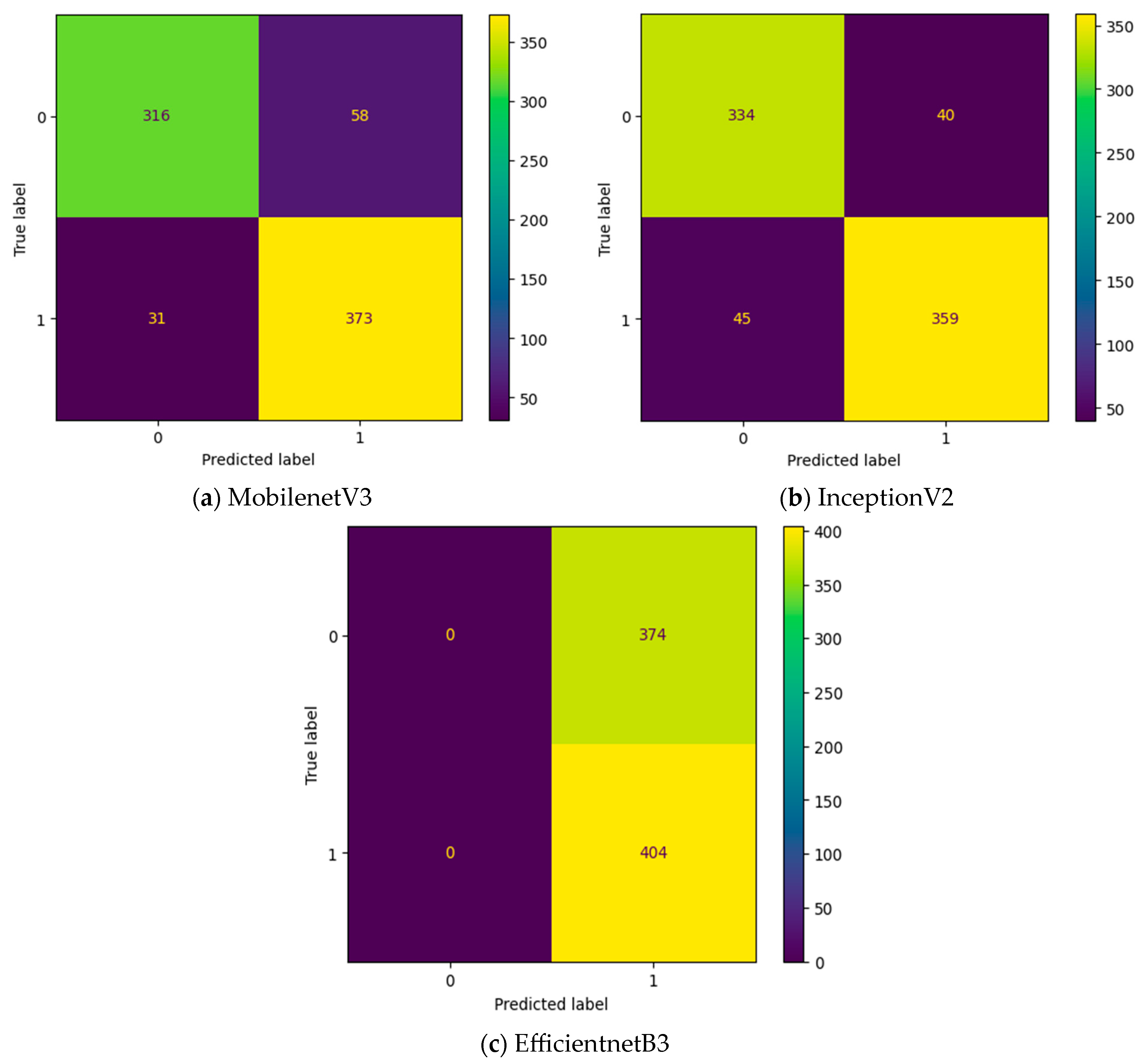
| Transfer Learning Model | Intermediate Layer | Accuracy | Precision | Recall | F1-Score |
|---|---|---|---|---|---|
| MobilenetV3 | NO | 0.89 | 0.87 | 0.92 | 0.89 |
| EfficientnetB3 | NO | 0.52 | 0.52 | 1 | 0.68 |
| InceptionV2 | NO | 0.88 | 0.89 | 0.88 | 0.88 |
| MobilenetV3 | PSO | 0.79 | 0.78 | 0.82 | 0.8 |
| EfficientnetB3 | PSO | 0.75 | 0.75 | 0.78 | 0.77 |
| InceptionV2 | PSO | 0.82 | 0.85 | 0.8 | 0.82 |
| MobilenetV3 | EHO | 0.77 | 0.77 | 0.8 | 0.79 |
| EfficientnetB3 | EHO | 0.8 | 0.82 | 0.78 | 0.8 |
| InceptionV2 | EHO | 0.83 | 0.85 | 0.82 | 0.83 |
| MobilenetV3 | GTO | 0.87 | 0.87 | 0.88 | 0.88 |
| EfficientnetB3 | GTO | 0.81 | 0.83 | 0.8 | 0.81 |
| InceptionV2 | GTO | 0.86 | 0.86 | 0.88 | 0.87 |
| MobilenetV3 | MGTO | 0.95 | 0.95 | 0.95 | 0.95 |
| EfficientnetB3 | MGTO | 0.9 | 0.92 | 0.9 | 0.91 |
| InceptionV2 | MGTO | 0.93 | 0.93 | 0.93 | 0.93 |
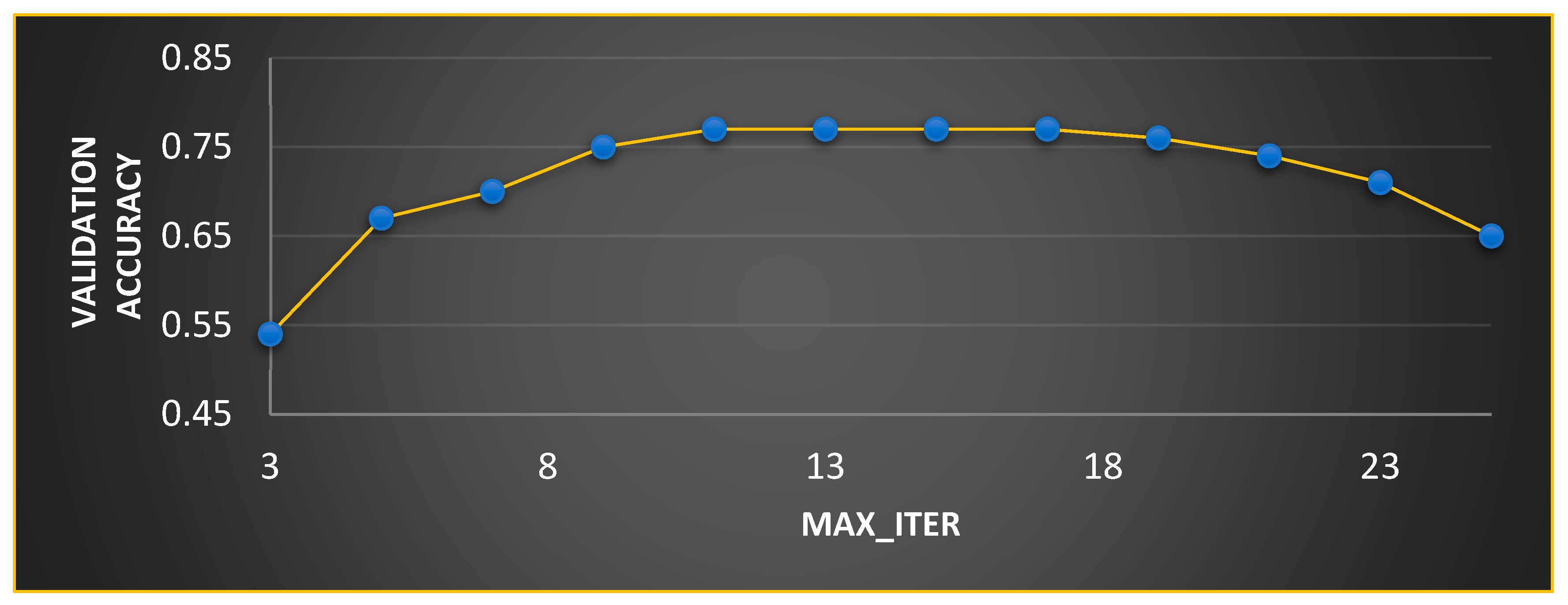
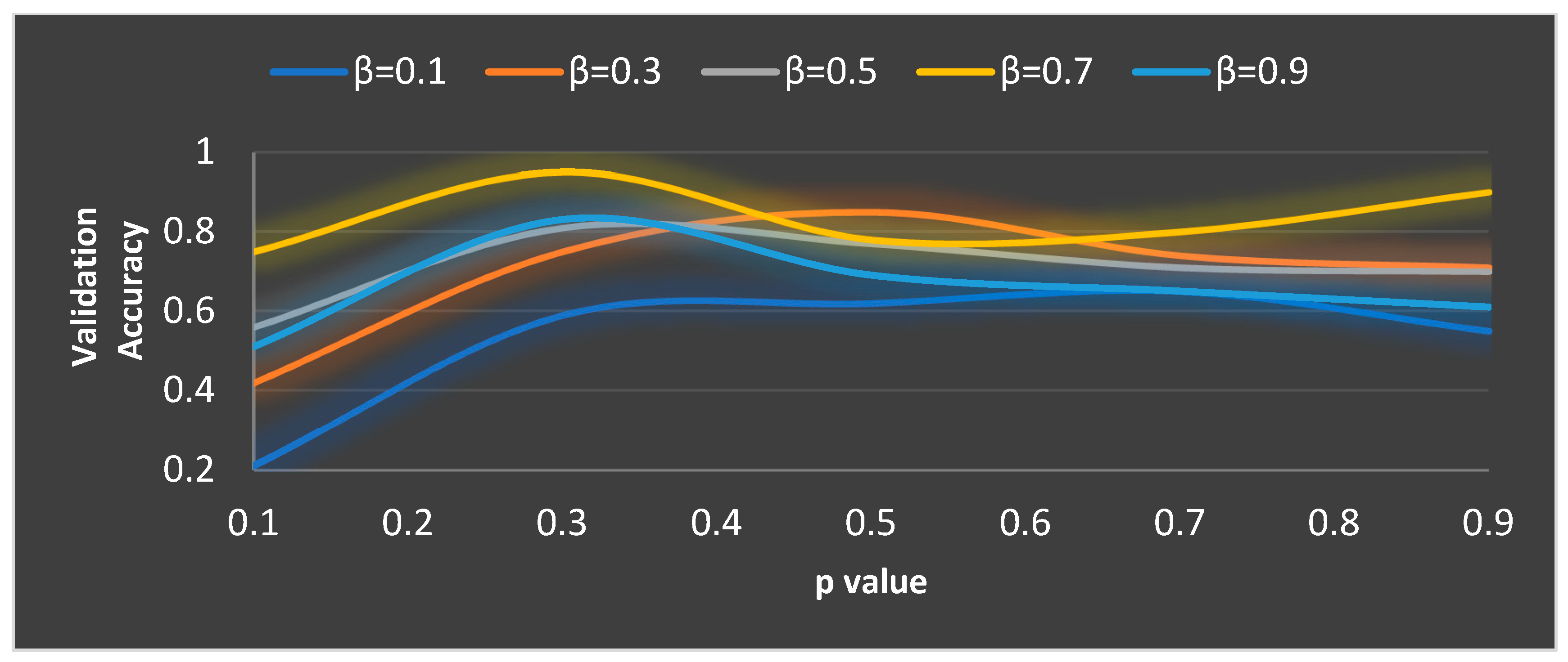
| Feature Extraction | Intermediate Layer | Ideal Parameter Values |
|---|---|---|
| MobilenetV3 | PSO | Max_Iter = 10, w = 0.6, c1 = 0.7, and c2 = 0.9 |
| EHO | Max_Iter = 12, = 0.9, and = 0.8 | |
| GTO | = 0.2, and = 0.7 | |
| MGTO | = 0.3, and = 0.7 | |
| EfficientnetB3 | PSO | Max_Iter = 12, w = 0.4, c1 = 0.7, and c2 = 0.9 |
| EHO | Max_Iter = 12, = 0.7, and = 0.8 | |
| GTO | = 0.5, and = 0.7 | |
| MGTO | = 0.3, and = 0.8 | |
| InceptionV2 | PSO | Max_Iter = 12, w = 0.6, c1 = 0.8, and c2 = 0.8 |
| EHO | Max_Iter = 11, = 0.8, and = 0.6 | |
| GTO | = 0.4, and = 0.7 | |
| MGTO | = 0.4, and = 0.6 |
| Transfer Learning Model | Intermediate Layer | Accuracy | Precision | Recall | F1-Score |
|---|---|---|---|---|---|
| MobilenetV3 | NO | 0.8 | 0.8 | 0.97 | 0.88 |
| EfficientnetB3 | NO | 0.74 | 0.74 | 1 | 0.85 |
| InceptionV2 | NO | 0.8 | 0.82 | 0.93 | 0.87 |
| MobilenetV3 | PSO | 0.78 | 0.81 | 0.92 | 0.86 |
| EfficientnetB3 | PSO | 0.75 | 0.79 | 0.9 | 0.84 |
| InceptionV2 | PSO | 0.8 | 0.81 | 0.95 | 0.87 |
| MobilenetV3 | EHO | 0.76 | 0.8 | 0.9 | 0.85 |
| EfficientnetB3 | EHO | 0.75 | 0.81 | 0.86 | 0.84 |
| InceptionV2 | EHO | 0.78 | 0.82 | 0.9 | 0.85 |
| MobilenetV3 | GTO | 0.82 | 0.82 | 0.98 | 0.89 |
| EfficientnetB3 | GTO | 0.78 | 0.81 | 0.92 | 0.86 |
| InceptionV2 | GTO | 0.82 | 0.83 | 0.97 | 0.89 |
| MobilenetV3 | MGTO | 0.88 | 0.88 | 0.97 | 0.92 |
| EfficientnetB3 | MGTO | 0.81 | 0.81 | 0.97 | 0.88 |
| InceptionV2 | MGTO | 0.86 | 0.84 | 1 | 0.91 |
| Transfer Learning Model | Intermediate Layer | Accuracy | Precision | Recall | F1-Score |
|---|---|---|---|---|---|
| MobilenetV3 | NO | 0.84 | 0.86 | 0.92 | 0.89 |
| EfficientnetB3 | NO | 0.71 | 0.71 | 1 | 0.83 |
| InceptionV2 | NO | 0.82 | 0.86 | 0.89 | 0.88 |
| MobilenetV3 | PSO | 0.78 | 0.84 | 0.85 | 0.85 |
| EfficientnetB3 | PSO | 0.73 | 0.81 | 0.81 | 0.81 |
| InceptionV2 | PSO | 0.78 | 0.83 | 0.87 | 0.85 |
| MobilenetV3 | EHO | 0.8 | 0.84 | 0.89 | 0.86 |
| EfficientnetB3 | EHO | 0.73 | 0.81 | 0.83 | 0.82 |
| InceptionV2 | EHO | 0.81 | 0.85 | 0.89 | 0.87 |
| MobilenetV3 | GTO | 0.91 | 0.92 | 0.96 | 0.94 |
| EfficientnetB3 | GTO | 0.75 | 0.83 | 0.83 | 0.83 |
| InceptionV2 | GTO | 0.86 | 0.87 | 0.95 | 0.9 |
| MobilenetV3 | MGTO | 0.94 | 0.97 | 0.85 | 0.96 |
| EfficientnetB3 | MGTO | 0.9 | 0.93 | 0.93 | 0.93 |
| InceptionV2 | MGTO | 0.93 | 0.97 | 0.93 | 0.95 |
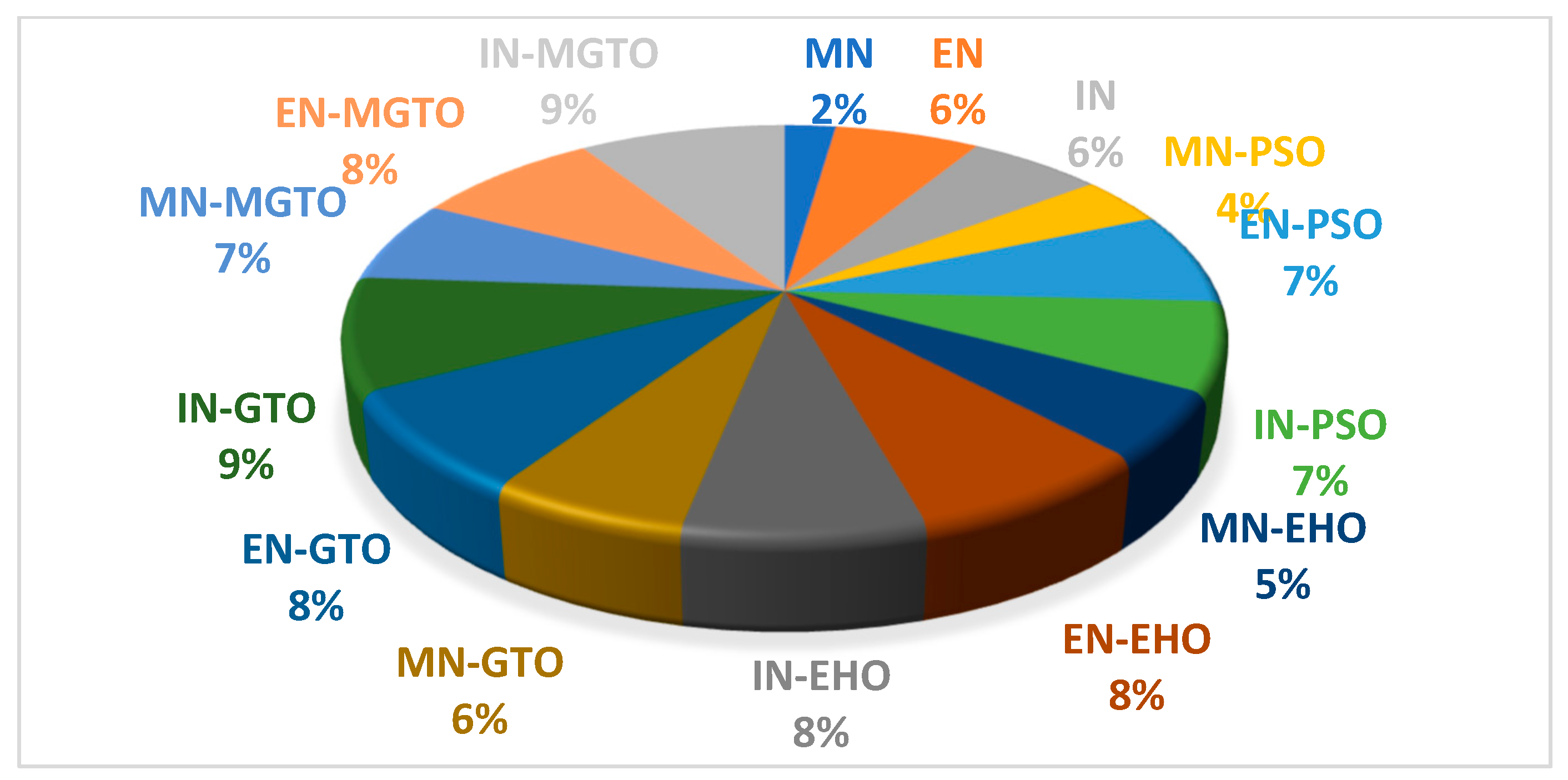
| DL Model | Training Time (hh:mm:ss) | DL Model | Training Time (hh:mm:ss) |
|---|---|---|---|
| MN | 00:05:33 | IN-EHO | 00:18:22 |
| EN | 00:15:42 | MN-GTO | 00:15:15 |
| IN | 00:14:37 | EN-GTO | 00:19:17 |
| MN-PSO | 00:09:23 | IN-GTO | 00:21:39 |
| EN-PSO | 00:17:52 | MN-MGTO | 00:15:52 |
| IN-PSO | 00:17:01 | EN-MGTO | 00:20:12 |
| MN-EHO | 00:12:47 | IN-MGTO | 00:22:21 |
| EN-EHO | 00:18:46 |
| Related Work | Year | Classification Framework | Accuracy (%) Attained |
|---|---|---|---|
| Rahman A.U. et al. [27] | 2022 | AlexNet | 90.06% |
| Aberville M. [52] | 2017 | Convolutional Neural Network | 88.3% |
| Alkhadar H. [53] | 2021 | KNN, Logistic Regression, Decision Tree, Random Forest | 76% |
| Alhazmi A. [54] | 2021 | Artificial Neural Network | 78.95% |
| Chu C.S. [55] | 2020 | SVM, KNN | 70.59% |
| Welikala R.A. [56] | 2020 | ResNet101 | 78.30% |
| Shavlokhova V. [57] | 2021 | CNN | 77.89% |
| Proposed | 2023 | Pre-trained MobileNetV3 for feature extraction and MGTO as an intermediate layer | 95% |
Disclaimer/Publisher’s Note: The statements, opinions and data contained in all publications are solely those of the individual author(s) and contributor(s) and not of MDPI and/or the editor(s). MDPI and/or the editor(s) disclaim responsibility for any injury to people or property resulting from any ideas, methods, instructions or products referred to in the content. |
© 2023 by the authors. Licensee MDPI, Basel, Switzerland. This article is an open access article distributed under the terms and conditions of the Creative Commons Attribution (CC BY) license (https://creativecommons.org/licenses/by/4.0/).
Share and Cite
Nagarajan, B.; Chakravarthy, S.; Venkatesan, V.K.; Ramakrishna, M.T.; Khan, S.B.; Basheer, S.; Albalawi, E. A Deep Learning Framework with an Intermediate Layer Using the Swarm Intelligence Optimizer for Diagnosing Oral Squamous Cell Carcinoma. Diagnostics 2023, 13, 3461. https://doi.org/10.3390/diagnostics13223461
Nagarajan B, Chakravarthy S, Venkatesan VK, Ramakrishna MT, Khan SB, Basheer S, Albalawi E. A Deep Learning Framework with an Intermediate Layer Using the Swarm Intelligence Optimizer for Diagnosing Oral Squamous Cell Carcinoma. Diagnostics. 2023; 13(22):3461. https://doi.org/10.3390/diagnostics13223461
Chicago/Turabian StyleNagarajan, Bharanidharan, Sannasi Chakravarthy, Vinoth Kumar Venkatesan, Mahesh Thyluru Ramakrishna, Surbhi Bhatia Khan, Shakila Basheer, and Eid Albalawi. 2023. "A Deep Learning Framework with an Intermediate Layer Using the Swarm Intelligence Optimizer for Diagnosing Oral Squamous Cell Carcinoma" Diagnostics 13, no. 22: 3461. https://doi.org/10.3390/diagnostics13223461
APA StyleNagarajan, B., Chakravarthy, S., Venkatesan, V. K., Ramakrishna, M. T., Khan, S. B., Basheer, S., & Albalawi, E. (2023). A Deep Learning Framework with an Intermediate Layer Using the Swarm Intelligence Optimizer for Diagnosing Oral Squamous Cell Carcinoma. Diagnostics, 13(22), 3461. https://doi.org/10.3390/diagnostics13223461