Automatic Detection and Classification of Diabetic Retinopathy Using the Improved Pooling Function in the Convolution Neural Network
Abstract
1. Introduction
2. Materials and Methods
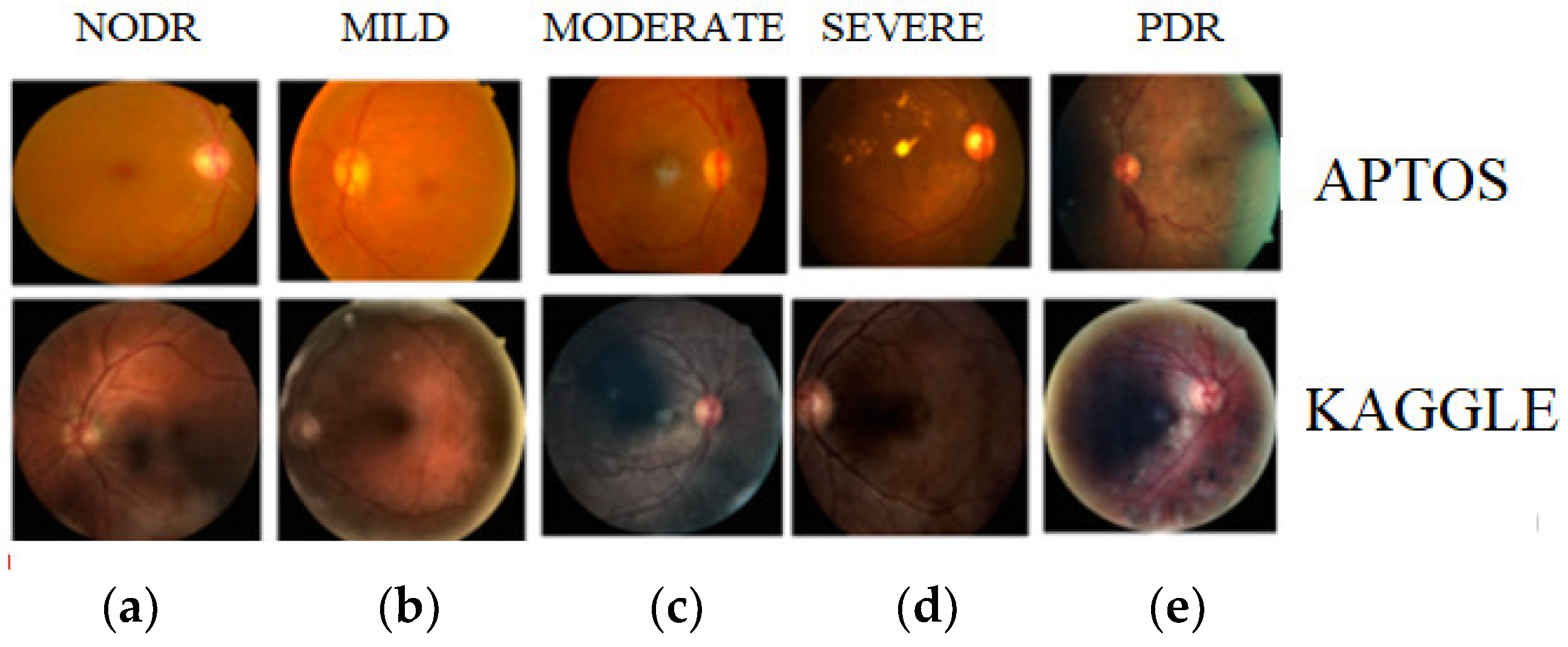
2.1. Dataset Collection
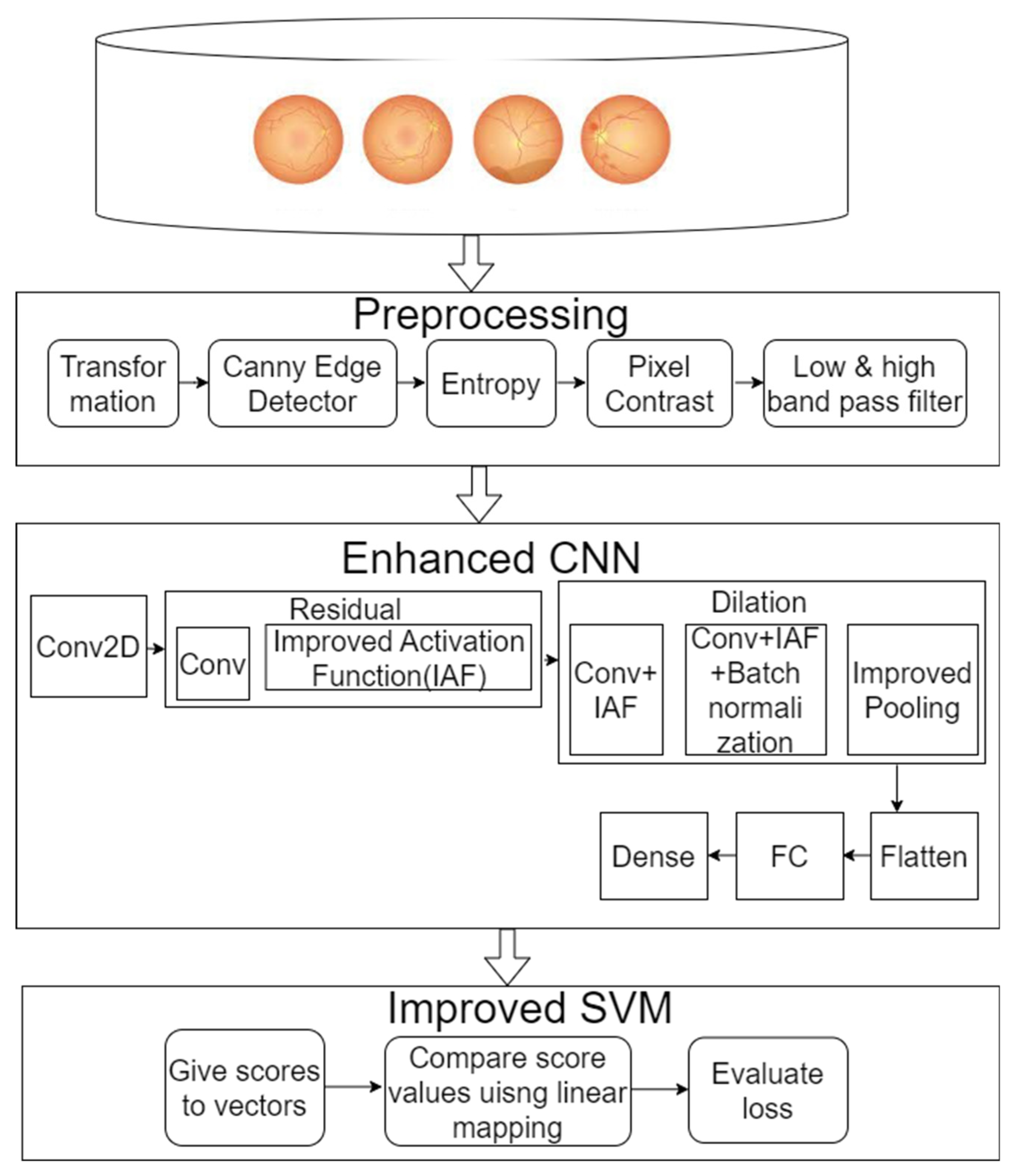
2.2. Pre-Processing
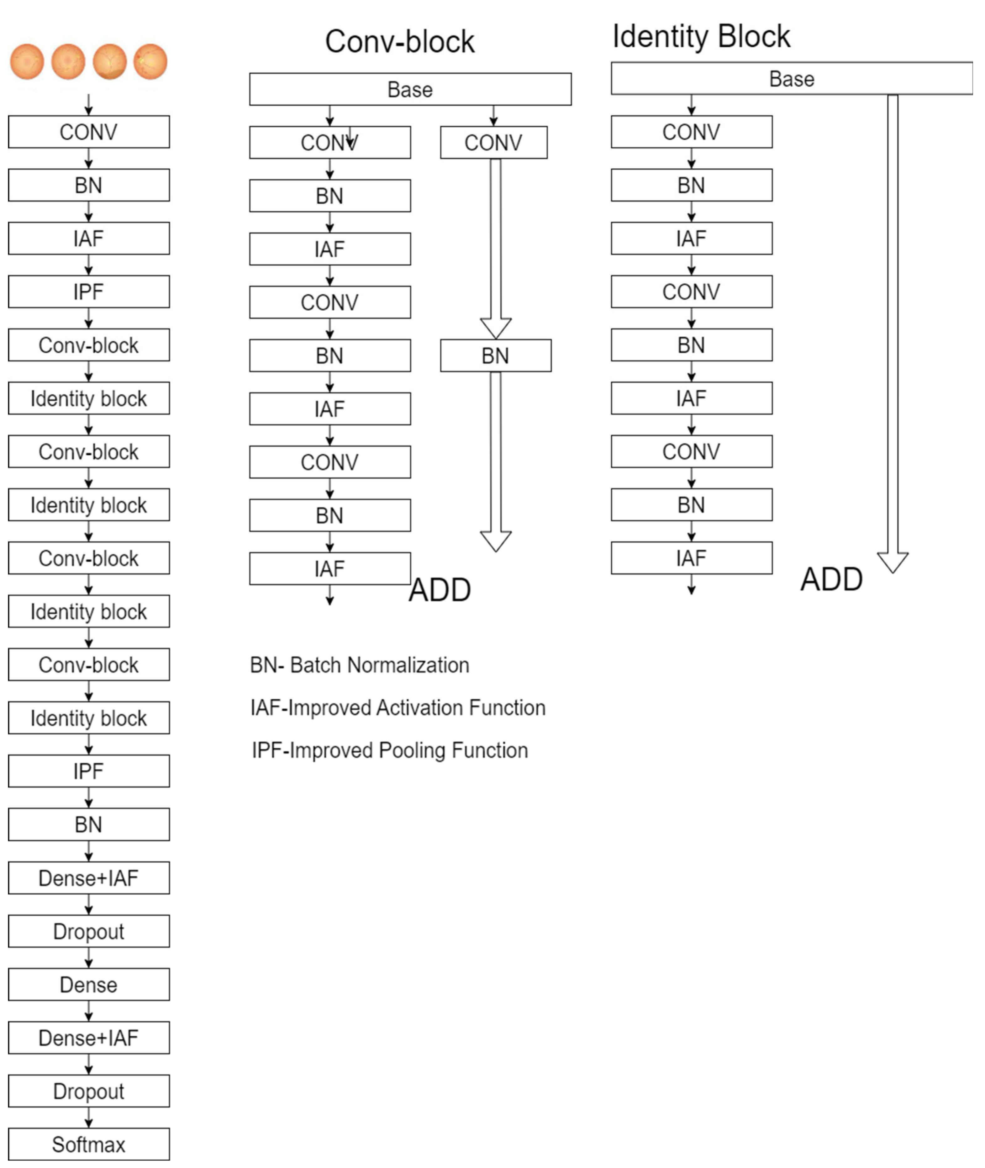
2.3. Enhanced ResNet-50
2.4. Classification
| Algorithm 1 Improved SVM |
Calculate the loss using the enhanced optimization for all values of j. Compare the extracted regions in the liver images. end
Compute the SVM argmax((w × p j) + b) end
|
3. Results
3.1. Image Enhancement Evaluation
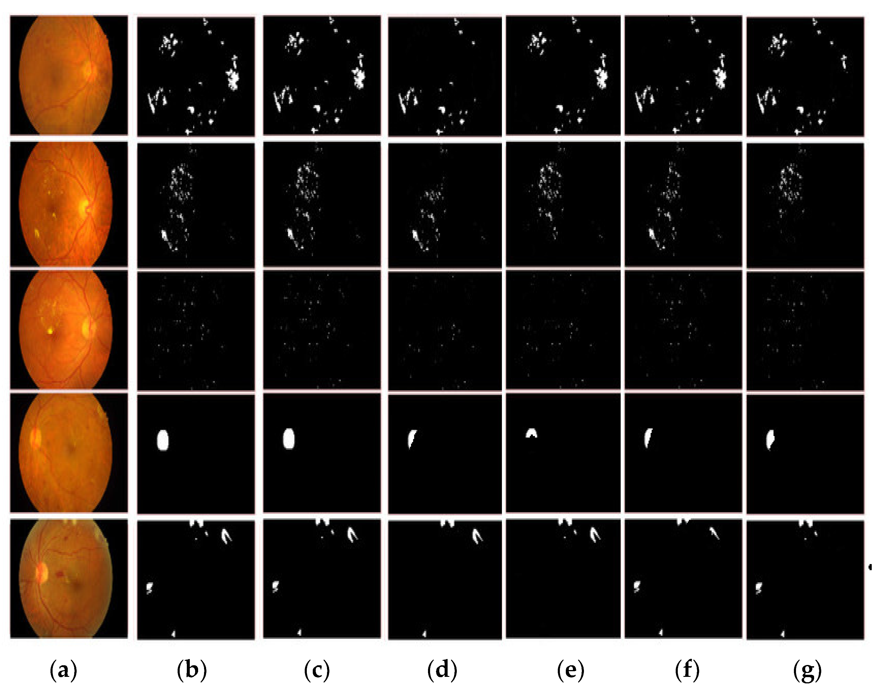
3.2. Segmentation Comparison
3.3. Evaluation of the APTOS Dataset
3.4. Evaluation of the Kaggle Dataset
4. Discussion
5. Conclusions
Author Contributions
Funding
Informed Consent Statement
Data Availability Statement
Conflicts of Interest
References
- Wild, S.H.; Roglic, G.; Green, A.; Sicree, R.; King, H. Global Prevalence of Diabetes: Estimates for the Year 2000 and Projections for 2030. Diabetes Care 2004, 27, 2569. [Google Scholar] [CrossRef]
- Scully, T. Diabetes in numbers. Nature 2012, 485, S2–S3. [Google Scholar] [CrossRef]
- Wu, L.; Fernandez-Loaiza, P.; Sauma, J.; Hernandez-Bogantes, E.; Masis, M. Classification of diabetic retinopathy and diabetic macula+r edema. World J. Diabetes 2013, 4, 290. [Google Scholar] [CrossRef]
- Khansari, M.M.; O’neill, W.D.; Penn, R.D.; Blair, N.P.; Shahidi, M. Detection of Subclinical Diabetic Retinopathy by Fine Structure Analysis of Retinal Images. J. Ophthalmol. 2019, 2019, 5171965. [Google Scholar] [CrossRef]
- Tufail, A.; Rudisill, C.; Egan, C.; Kapetanakis, V.V.; Salas-Vega, S.; Owen, C.G.; Rudnicka, A.R. Automated diabetic retinopathy image assessment software: Diagnostic accuracy and cost-effectiveness compared with human graders. Ophthalmology 2017, 124, 343–351. [Google Scholar] [CrossRef]
- Gulshan, V.; Rajan, R.; Widner, K.; Wu, D.; Wubbels, P.; Rhodes, T.; Whitehouse, K.; Coram, M.; Corrado, G.; Ramasamy, K.; et al. Performance of a Deep-Learning Algorithm vs Manual Grading for Detecting Diabetic Retinopathy in India. JAMA Ophthalmol. 2019, 137, 987–993. [Google Scholar] [CrossRef]
- García, G.; Gallardo, J.; Mauricio, A.; López, J.; Del Carpio, C. Detection of diabetic retinopathy based on a convolutional neural network using retinal fundus images. In Artificial Neural Networks and Machine Learning–ICANN 2017, Proceedings of the 26th International Conference on Artificial Neural Networks, Alghero, Italy, 11–14 September 2017; Springer International Publishing: Cham, Switzerland, 2017; pp. 635–642, Proceedings, Part II 26. [Google Scholar]
- Hemanth, D.J.; Deperlioglu, O.; Kose, U. An enhanced diabetic retinopathy detection and classification approach using deep convolutional neural network. Neural Comput. Appl. 2019, 32, 707–721. [Google Scholar] [CrossRef]
- Qummar, S.; Khan, F.G.; Shah, S.; Khan, A.; Shamshirband, S.; Rehman, Z.U.; Khan, I.A.; Jadoon, W. A Deep Learning Ensemble Approach for Diabetic Retinopathy Detection. IEEE Access 2019, 7, 150530–150539. [Google Scholar] [CrossRef]
- Costa, P.; Galdran, A.; Smailagic, A.; Campilho, A. A Weakly-Supervised Framework for Interpretable Diabetic Retinopathy Detection on Retinal Images. IEEE Access 2018, 6, 18747–18758. [Google Scholar] [CrossRef]
- Wan, S.; Liang, Y.; Zhang, Y. Deep convolutional neural networks for diabetic retinopathy detection by image classification. Comput. Electr. Eng. 2018, 72, 274–282. [Google Scholar] [CrossRef]
- Bhatkar, A.P.; Kharat, G.U. Detection of diabetic retinopathy in retinal images using MLP classifier. In Proceedings of the 2015 IEEE International Symposium on Nanoelectronic and Information Systems, Indore, India, 21–23 December 2015; IEEE: New York, NY, USA, 2015; pp. 331–335. [Google Scholar]
- Xu, J.; Zhang, X.; Chen, H.; Li, J.; Zhang, J.; Shao, L.; Wang, G. Automatic Analysis of Microaneurysms Turnover to Diagnose the Progression of Diabetic Retinopathy. IEEE Access 2018, 6, 9632–9642. [Google Scholar] [CrossRef]
- Antal, B.; Hajdu, A. An Ensemble-Based System for Microaneurysm Detection and Diabetic Retinopathy Grading. IEEE Trans. Biomed. Eng. 2012, 59, 1720–1726. [Google Scholar] [CrossRef]
- Dutta, S.; Manideep, B.C.; Basha, S.M.; Caytiles, R.D.; Iyengar, N.C.S.N. Classification of Diabetic Retinopathy Images by Using Deep Learning Models. Int. J. Grid Distrib. Comput. 2018, 11, 99–106. [Google Scholar] [CrossRef]
- Lunscher, N.; Chen, M.L.; Jiang, N.; Zelek, J. Automated Screening for Diabetic Retinopathy Using Compact Deep Networks. J. Comput. Vis. Imaging Syst. 2017, 3, 1–3. [Google Scholar] [CrossRef]
- Available online: https://www.kaggle.com/competitions/aptos2019-blindness-detection/data (accessed on 2 October 2022).
- Available online: https://www.kaggle.com/competitions/diabetic-retinopathy-detection/discussion/234309 (accessed on 2 October 2022).
- Nirthika, R.; Manivannan, S.; Ramanan, A.; Wang, R. Pooling in convolutional neural networks for medical image analysis: A survey and an empirical study. Neural Comput. Appl. 2022, 34, 5321–5347. [Google Scholar] [CrossRef]
- Yamashita, R.; Nishio, M.; Do, R.K.G.; Togashi, K. Convolutional neural networks: An overview and application in radiology. Insights Imaging 2018, 9, 611–629. [Google Scholar] [CrossRef]
- Kumar, M.; Bhandari, A.K. Contrast Enhancement Using Novel White Balancing Parameter Optimization for Perceptually Invisible Images. IEEE Trans. Image Process. 2020, 29, 7525–7536. [Google Scholar] [CrossRef]
- Niu, Y.; Wu, X.; Shi, G. Image Enhancement by Entropy Maximization and Quantization Resolution Upconversion. IEEE Trans. Image Process. 2016, 25, 4815–4828. [Google Scholar] [CrossRef]
- Veluchamy, M.; Bhandari, A.K.; Subramani, B. Optimized Bezier Curve Based Intensity Mapping Scheme for Low Light Image Enhancement. IEEE Trans. Emerg. Top. Comput. Intell. 2021, 6, 602–612. [Google Scholar] [CrossRef]
- Pizer, S.M. Contrast-limited adaptive histogram equalization: Speed and effectiveness stephen m. pizer, r. eugene johnston, james p. ericksen, bonnie c. yankaskas, keith e. muller medical image display research group. In Proceedings of the First Conference on Visualization in Biomedical Computing, Atlanta, GA, USA, 22–25 May 1990; Volume 337, p. 2. [Google Scholar]
- Singh, K.; Kapoor, R. Image enhancement using Exposure based Sub Image Histogram Equalization. Pattern Recognit. Lett. 2014, 36, 10–14. [Google Scholar] [CrossRef]
- Kansal, S.; Tripathi, R.K. New adaptive histogram equalisation heuristic approach for contrast enhancement. IET Image Process. 2020, 14, 1110–1119. [Google Scholar] [CrossRef]
- Yang, K.-F.; Zhang, X.-S.; Li, Y.-J. A Biological Vision Inspired Framework for Image Enhancement in Poor Visibility Conditions. IEEE Trans. Image Process. 2019, 29, 1493–1506. [Google Scholar] [CrossRef]
- Arici, T.; Dikbas, S.; Altunbasak, Y. A Histogram Modification Framework and Its Application for Image Contrast Enhance-ment. IEEE Trans. Image Process. 2009, 18, 1921–1935. [Google Scholar] [CrossRef]
- Mishra, M.; Menon, H.; Mukherjee, A. Characterization of S1 and S2 Heart Sounds Using Stacked Autoencoder and Convo-lutional Neural Network. IEEE Trans. Instrum. Meas. 2018, 68, 3211–3220. [Google Scholar] [CrossRef]
- Simonyan, K.; Zisserman, A. Very deep convolutional networks for large-scale image recognition. arXiv 2014, arXiv:1409.1556. [Google Scholar]
- Li, H.-Y.; Dong, L.; Zhou, W.-D.; Wu, H.-T.; Zhang, R.-H.; Li, Y.-T.; Yu, C.-Y.; Wei, W.-B. Development and validation of medical record-based logistic regression and machine learning models to diagnose diabetic retinopathy. Graefe’s Arch. Clin. Exp. Ophthalmol. 2022, 261, 681–689. [Google Scholar] [CrossRef]
- Tsao, H.Y.; Chan, P.Y.; Su, E.C.Y. Predicting diabetic retinopathy and identifying interpretable biomedical features using machine learning algorithms. BMC Bioinform. 2018, 19, 111–121. [Google Scholar] [CrossRef]
- Bhatia, K.; Arora, S.; Tomar, R. Diagnosis of diabetic retinopathy using machine learning classification algorithm. In Proceedings of the 2016 2nd International Conference on Next Generation Computing Technologies (NGCT), Dehradun, India, 14–16 October 2016; IEEE: New York, NY, USA, 2016; pp. 347–351. [Google Scholar]
- Chen, Y.; Hu, X.; Fan, W.; Shen, L.; Zhang, Z.; Liu, X.; Du, J.; Li, H.; Chen, Y.; Li, H. Fast density peak clustering for large scale data based on kNN. Knowl.-Based Syst. 2019, 187, 104824. [Google Scholar] [CrossRef]
- Cao, K.; Xu, J.; Zhao, W.Q. Artificial intelligence on diabetic retinopathy diagnosis: An automatic classification method based on grey level co-occurrence matrix and naive Bayesian model. Int. J. Ophthalmol. 2019, 12, 1158. [Google Scholar] [CrossRef]
- Alzami, F.; Megantara, R.A.; Fanani, A.Z. Diabetic retinopathy grade classification based on fractal analysis and random forest. In Proceedings of the 2019 International Seminar on Application for Technology of Information and Communication (iSemantic), Se-marang, Indonesia, 21–22 September 2019; IEEE: New York, NY, USA, 2019; pp. 272–276. [Google Scholar]
- Yu, S.; Tan, K.K.; Sng, B.L.; Li, S.; Sia, A.T.H. Lumbar Ultrasound Image Feature Extraction and Classification with Support Vector Machine. Ultrasound Med. Biol. 2015, 41, 2677–2689. [Google Scholar] [CrossRef]
- Seoud, L.; Chelbi, J.; Cheriet, F. Automatic grading of diabetic retinopathy on a public database. In Proceedings of the Ophthalmic Medical Image Analysis International Workshop, Munich, Germany, 8 October 2015; University of Iowa: Iowa City, IA, USA, 2015; Volume 2. No. 2015. [Google Scholar]
- Savarkar, S.P.; Kalkar, N.; Tade, S.L. Diabetic retinopathy using image processing detection, classification and analysis. Int. J. Adv. Comput. Res. 2013, 3, 285. [Google Scholar]
- Gondal, W.M.; Kohler, J.M.; Grzeszick, R.; Fink, G.A.; Hirsch, M. Weakly-supervised localization of diabetic retinopathy lesions in retinal fundus images. In Proceedings of the 2017 IEEE International Conference on Image Processing (ICIP), Beijing, China, 17–20 September 2017; pp. 2069–2073. [Google Scholar] [CrossRef]
- Wang, Z.; Yin, Y.; Shi, J.; Fang, W.; Li, H.; Wang, X. Zoom-in-net: Deep mining lesions for diabetic retinopathy detection. In Medical Image Computing and Computer Assisted Intervention—MICCAI 2017, Proceedings of the 20th International Conference, Quebec City, QC, Canada, 11–13 September 2017; Springer International Publishing: Cham, Switzerland, 2017; pp. 267–275, Proceedings, Part III 20. [Google Scholar]
- Chandrakumar, T.; Kathirvel, R.J.I.J.E.R.T. Classifying diabetic retinopathy using deep learning architecture. Int. J. Eng. Res. Technol. 2016, 5, 19–24. [Google Scholar]
- Yang, Y.; Li, T.; Li, W.; Wu, H.; Fan, W.; Zhang, W. Lesion detection and grading of diabetic retinopathy via two-stages deep convolutional neural networks. In Medical Image Computing and Computer Assisted Intervention—MICCAI 2017, Proceedings of the 20th International Conference, Quebec City, QC, Canada, 11–13 September 2017; Springer International Publishing: Cham, Swit-zerland, 2017; pp. 533–540, Proceedings, Part III 20. [Google Scholar]


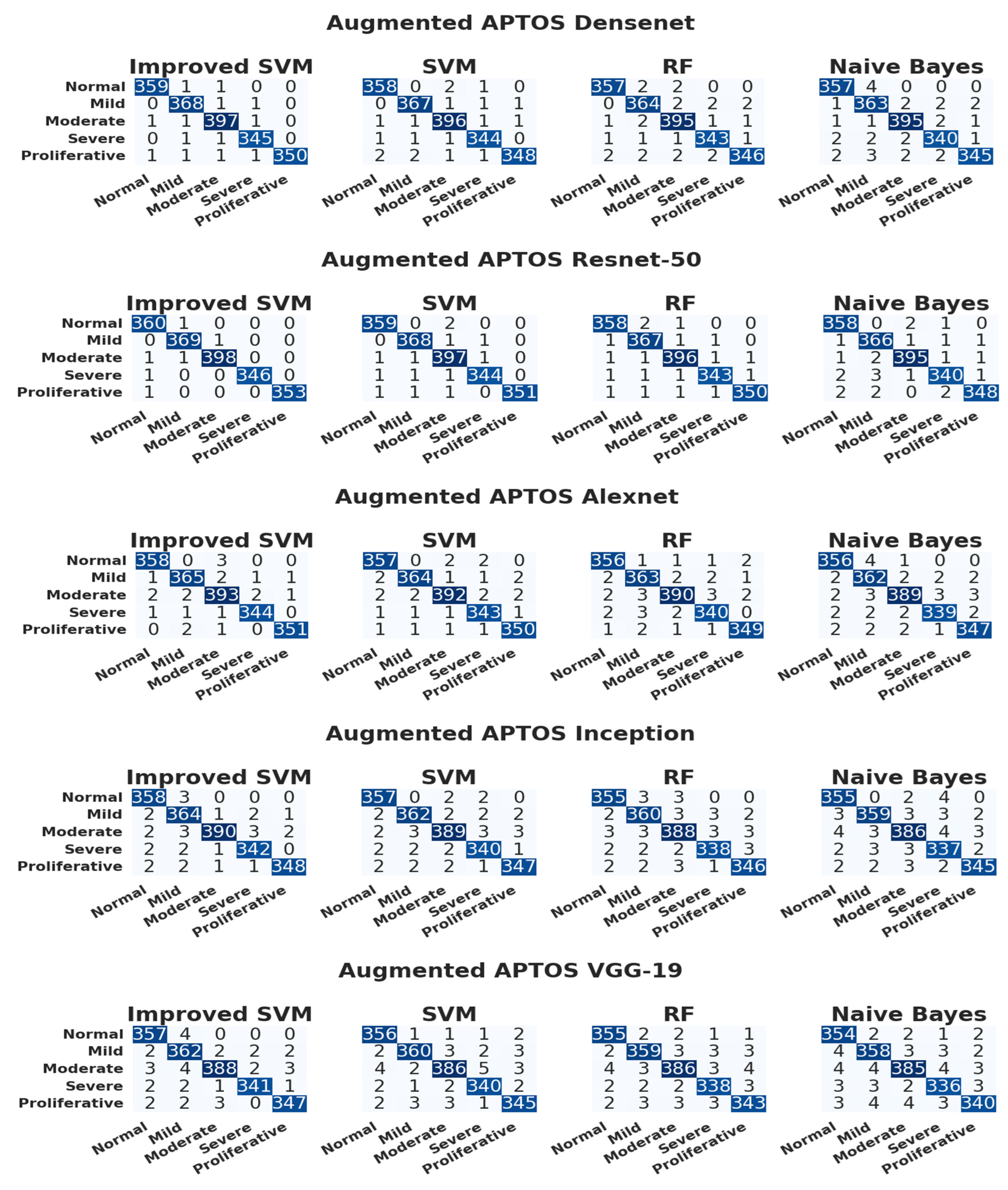
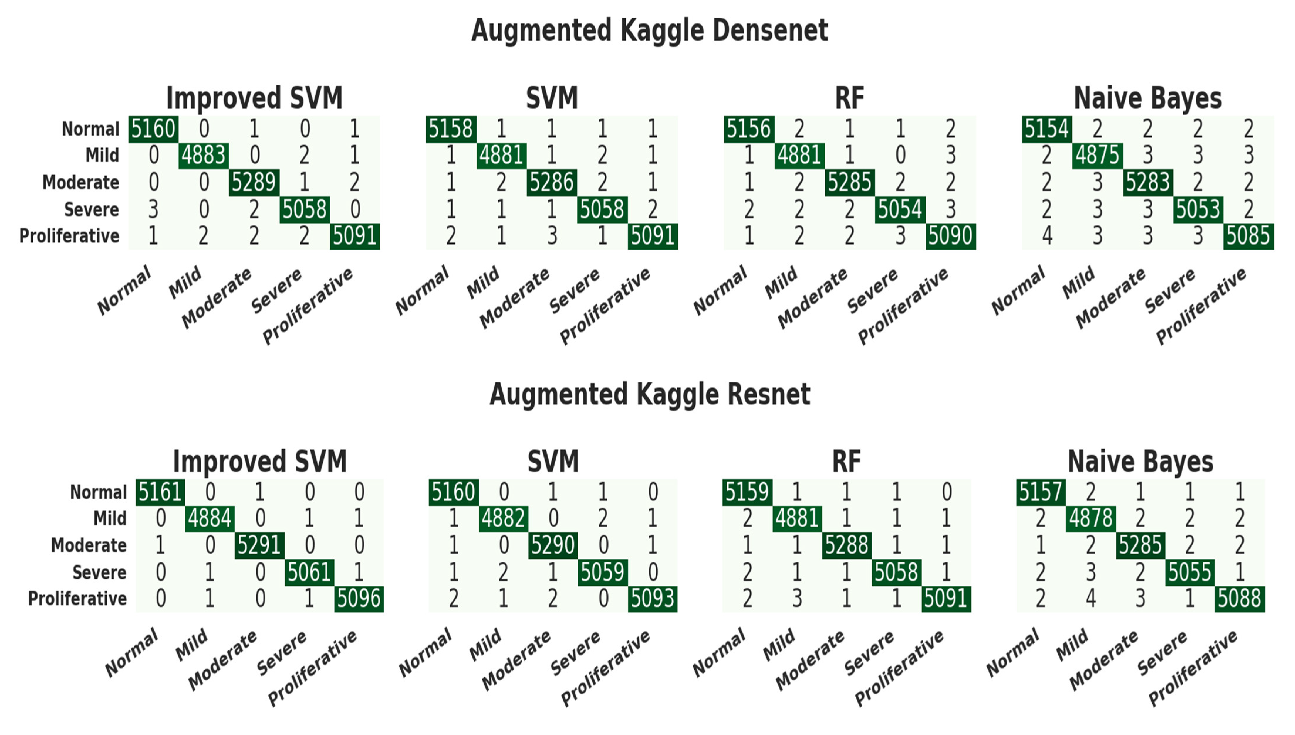
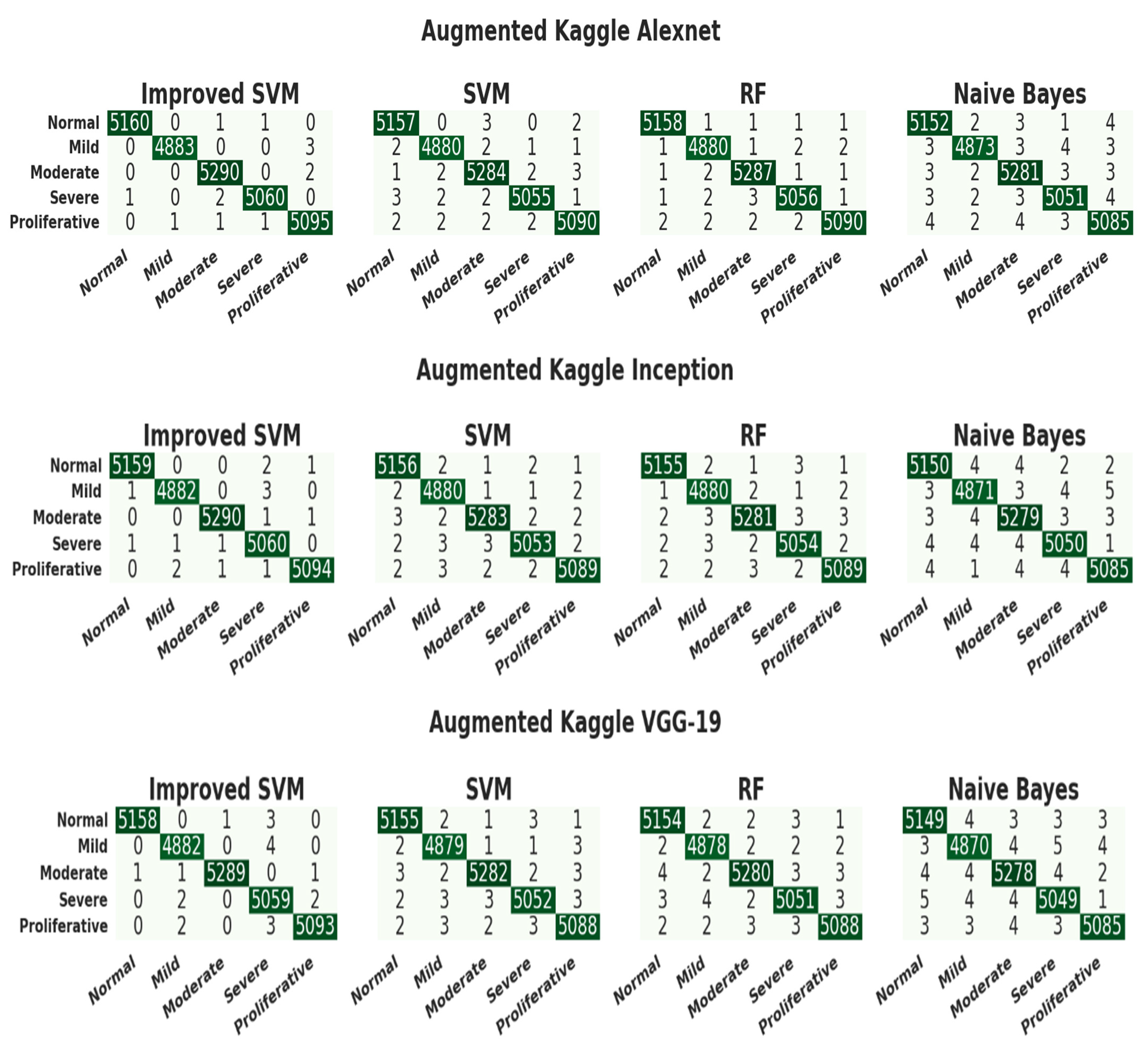
| Dataset | NODR | Mild DR | Moderate DR | Severe DR | PDR | Count |
|---|---|---|---|---|---|---|
| APTOS | 1805 | 370 | 999 | 193 | 295 | 3662 |
| Kaggle | 25,810 | 2443 | 5292 | 873 | 708 | 35,126 |
| Class | APTOS | Kaggle | ||||
|---|---|---|---|---|---|---|
| Original | Operations | Augmented | Original | Operations | Augmented | |
| NoDR | 1805 | 0 | 1805 | 25,810 | 0 | 25,810 |
| MildDR | 370 | 5 | 1850 | 2443 | 10 | 24,430 |
| Moderate DR | 999 | 2 | 1998 | 5292 | 5 | 26,460 |
| Severe DR | 193 | 9 | 1737 | 873 | 29 | 25,317 |
| PDR | 295 | 6 | 1770 | 708 | 36 | 25,488 |
| Total | 3662 | 9160 | 35,126 | 127,505 | ||
| Class | APTOS | Kaggle | ||
|---|---|---|---|---|
| Training | Testing | Training | Testing | |
| NoDR | 1444 | 361 | 20,648 | 5162 |
| MildDR | 1480 | 370 | 19,544 | 4886 |
| Moderate DR | 1598 | 400 | 21,166 | 5292 |
| Severe DR | 1390 | 347 | 20,254 | 5063 |
| PDR | 1416 | 354 | 20,390 | 5098 |
| Total | 7328 | 1832 | 102,004 | 25,501 |
| Model | PSNR | GMSD | Entropy | SSIM | PCQI | Processing Time (s) |
|---|---|---|---|---|---|---|
| Clahe [24] | 30.83 | 0.163 | 7.263 | 0.634 | 1.139 | 0.155 |
| ESIHE [25] | 31.93 | 0.074 | 7.316 | 0.635 | 1.282 | 0.153 |
| HAHE [26] | 32.82 | 0.125 | 7.226 | 0.693 | 1.001 | 0.373 |
| BIMEF [27] | 31.68 | 0.199 | 7.269 | 0.736 | 1.007 | 0.364 |
| HMF [28] | 32.63 | 0.085 | 7.283 | 0.636 | 1.103 | 0.218 |
| ABC | 34.83 | 0.048 | 7.834 | 0.877 | 1.378 | 0.173 |
| Proposed | 35.56 | 0.037 | 7.935 | 0.983 | 1.484 | 0.151 |
| Model | Pool + Act | Accuracy | Precision | Recall |
|---|---|---|---|---|
| DenseNet [29] | Max + Relu | 0.9484 | 0.8364 | 0.9584 |
| Inception [12] | Max + Relu | 0.9847 | 0.8578 | 0.9848 |
| VGG-19 [30] | Max + Relu | 0.9795 | 0.8479 | 0.9483 |
| AlexNet [31] | Max + Relu | 0.9858 | 0.9378 | 0.9847 |
| ResNet-50 | Proposed | 0.9986 | 1.0000 | 1.0000 |
| AlexNet | Proposed | 0.9986 | 1.0000 | 0.9864 |
| DenseNet | Proposed | 0.9959 | 1.0000 | 0.9916 |
| Inception | Proposed | 0.9972 | 0.9864 | 0.9864 |
| VGG-19 | Proposed | 0.9986 | 0.9866 | 1.0000 |
| CNN Model | Classifier | Accuracy | Precision | Recall | F1-Score | Class |
|---|---|---|---|---|---|---|
| DenseNet | ISVM | 0.99781659 | 0.99445983 | 0.99445983 | 0.99445983 | Normal |
| 0.99672489 | 0.98924731 | 0.99459459 | 0.99191375 | Mild | ||
| 0.99617904 | 0.99002494 | 0.99250000 | 0.99126092 | Moderate | ||
| 0.99727074 | 0.99137931 | 0.99423631 | 0.99280576 | Severe | ||
| 0.99781659 | 1.0000000 | 0.98870056 | 0.99431818 | PDR | ||
| SVM | 0.99617904 | 0.98895028 | 0.99168975 | 0.99031812 | Normal | |
| 0.99617904 | 0.98921833 | 0.99189189 | 0.99055331 | Mild | ||
| 0.99508734 | 0.98753117 | 0.99000000 | 0.98876404 | Moderate | ||
| 0.99617904 | 0.98850575 | 0.99135447 | 0.98992806 | Severe | ||
| 0.99563319 | 0.99428571 | 0.98305085 | 0.98863636 | PDR | ||
| RF | 0.99563319 | 0.98891967 | 0.98891967 | 0.98891967 | Normal | |
| 0.99290393 | 0.98113208 | 0.98378378 | 0.98245614 | Mild | ||
| 0.99344978 | 0.98258706 | 0.98750000 | 0.98503741 | Moderate | ||
| 0.99508734 | 0.98563218 | 0.98847262 | 0.98705036 | Severe | ||
| 0.99344978 | 0.98857143 | 0.97740113 | 0.98295455 | PDR | ||
| NB | 0.99454148 | 0.98347107 | 0.98891967 | 0.98618785 | Normal | |
| 0.99072052 | 0.97319035 | 0.98108108 | 0.97711978 | Mild | ||
| 0.99399563 | 0.98503741 | 0.98750000 | 0.98626717 | Moderate | ||
| 0.99290393 | 0.98265896 | 0.97982709 | 0.98124098 | Severe | ||
| 0.99290393 | 0.98853868 | 0.97457627 | 0.98150782 | PDR | ||
| ResNet-50 | ISVM | 0.99781659 | 0.99173554 | 0.99722992 | 0.99447514 | Normal |
| 0.99836245 | 0.99460916 | 0.9972973 | 0.99595142 | Mild | ||
| 0.99836245 | 0.99749373 | 0.9950000 | 0.99624531 | Moderate | ||
| 0.99945415 | 1.00000000 | 0.99711816 | 0.99855700 | Severe | ||
| 0.99945415 | 1.00000000 | 0.99717514 | 0.99858557 | PDR | ||
| SVM | 0.99727074 | 0.99171271 | 0.99445983 | 0.99308437 | Normal | |
| 0.99727074 | 0.99191375 | 0.99459459 | 0.99325236 | Mild | ||
| 0.99563319 | 0.98756219 | 0.99250000 | 0.99002494 | Moderate | ||
| 0.99727074 | 0.99421965 | 0.99135447 | 0.99278499 | Severe | ||
| 0.99836245 | 1.00000000 | 0.99152542 | 0.99574468 | PDR | ||
| RF | 0.99617904 | 0.98895028 | 0.99168975 | 0.99031812 | Normal | |
| 0.99563319 | 0.98655914 | 0.99189189 | 0.98921833 | Mild | ||
| 0.99563319 | 0.99000000 | 0.99000000 | 0.99000000 | Moderate | ||
| 0.99617904 | 0.99132948 | 0.98847262 | 0.98989899 | Severe | ||
| 0.99672489 | 0.99431818 | 0.98870056 | 0.99150142 | PDR | ||
| NB | 0.99508734 | 0.98351648 | 0.99168975 | 0.98758621 | Normal | |
| 0.99399563 | 0.98123324 | 0.98918919 | 0.98519515 | Mild | ||
| 0.99508734 | 0.98997494 | 0.98750000 | 0.98873592 | Moderate | ||
| 0.99344978 | 0.98550725 | 0.97982709 | 0.98265896 | Severe | ||
| 0.99508734 | 0.99145299 | 0.98305085 | 0.98723404 | PDR | ||
| AlexNet | ISVM | 0.99617904 | 0.98895028 | 0.99168975 | 0.99031812 | Normal |
| 0.99454148 | 0.98648649 | 0.98648649 | 0.98648649 | Mild | ||
| 0.99235808 | 0.98250000 | 0.98250000 | 0.98250000 | Moderate | ||
| 0.99672489 | 0.99135447 | 0.99135447 | 0.99135447 | Severe | ||
| 0.99727074 | 0.99433428 | 0.99152542 | 0.99292786 | PDR | ||
| SVM | 0.99454148 | 0.98347107 | 0.98891967 | 0.98618785 | Normal | |
| 0.99454148 | 0.98913043 | 0.98378378 | 0.98644986 | Mild | ||
| 0.99290393 | 0.98740554 | 0.98000000 | 0.98368883 | Moderate | ||
| 0.99454148 | 0.98280802 | 0.98847262 | 0.98563218 | Severe | ||
| 0.99508734 | 0.98591549 | 0.98870056 | 0.98730606 | PDR | ||
| RF | 0.99344978 | 0.98071625 | 0.98614958 | 0.98342541 | Normal | |
| 0.99126638 | 0.97580645 | 0.98108108 | 0.97843666 | Mild | ||
| 0.99126638 | 0.98484848 | 0.97500000 | 0.97989950 | Moderate | ||
| 0.99235808 | 0.97982709 | 0.97982709 | 0.97982709 | Severe | ||
| 0.99454148 | 0.98587571 | 0.98587571 | 0.98587571 | PDR | ||
| NB | 0.99290393 | 0.97802198 | 0.98614958 | 0.98206897 | Normal | |
| 0.98962882 | 0.97050938 | 0.97837838 | 0.97442799 | Mild | ||
| 0.99017467 | 0.98232323 | 0.97250000 | 0.97738693 | Moderate | ||
| 0.99235808 | 0.9826087 | 0.97694524 | 0.97976879 | Severe | ||
| 0.99235808 | 0.98022599 | 0.98022599 | 0.98022599 | PDR | ||
| Inception | ISVM | 0.99399563 | 0.97814208 | 0.99168975 | 0.98486933 | Normal |
| 0.99126638 | 0.97326203 | 0.98378378 | 0.97849462 | Mild | ||
| 0.99290393 | 0.99236641 | 0.97500000 | 0.98360656 | Moderate | ||
| 0.99399563 | 0.98275862 | 0.98559078 | 0.98417266 | Severe | ||
| 0.99508734 | 0.99145299 | 0.98305085 | 0.98723404 | PDR | ||
| SVM | 0.99344978 | 0.97808219 | 0.98891967 | 0.98347107 | Normal | |
| 0.99181223 | 0.98102981 | 0.97837838 | 0.97970230 | Mild | ||
| 0.98962882 | 0.97984887 | 0.97250000 | 0.97616060 | Moderate | ||
| 0.99181223 | 0.97701149 | 0.97982709 | 0.97841727 | Severe | ||
| 0.99290393 | 0.98300283 | 0.98022599 | 0.98161245 | PDR | ||
| RF | 0.99181223 | 0.97527473 | 0.98337950 | 0.97931034 | Normal | |
| 0.98908297 | 0.97297297 | 0.97297297 | 0.97297297 | Mild | ||
| 0.98744541 | 0.97243108 | 0.9700000 | 0.97121402 | Moderate | ||
| 0.99126638 | 0.97971014 | 0.9740634 | 0.97687861 | Severe | ||
| 0.99126638 | 0.97740113 | 0.97740113 | 0.97740113 | PDR | ||
| NB | 0.99072052 | 0.96994536 | 0.98337950 | 0.97661623 | Normal | |
| 0.98962882 | 0.97820163 | 0.97027027 | 0.97421981 | Mild | ||
| 0.98635371 | 0.97229219 | 0.96500000 | 0.96863237 | Moderate | ||
| 0.98744541 | 0.96285714 | 0.97118156 | 0.96700143 | Severe | ||
| 0.99126638 | 0.98011364 | 0.97457627 | 0.97733711 | PDR | ||
| VGG-19 | ISVM | 0.99290393 | 0.97540984 | 0.98891967 | 0.98211829 | Normal |
| 0.98908297 | 0.96791444 | 0.97837838 | 0.97311828 | Mild | ||
| 0.99017467 | 0.98477157 | 0.97000000 | 0.97732997 | Moderate | ||
| 0.99454148 | 0.98840580 | 0.98270893 | 0.98554913 | Severe | ||
| 0.99290393 | 0.98300283 | 0.98022599 | 0.98161245 | PDR | ||
| SVM | 0.99181223 | 0.97267760 | 0.98614958 | 0.97936726 | Normal | |
| 0.99072052 | 0.98092643 | 0.97297297 | 0.97693351 | Mild | ||
| 0.98744541 | 0.97721519 | 0.96500000 | 0.97106918 | Moderate | ||
| 0.99126638 | 0.97421203 | 0.97982709 | 0.97701149 | Severe | ||
| 0.98962882 | 0.97183099 | 0.97457627 | 0.97320169 | PDR | ||
| RF | 0.99126638 | 0.97260274 | 0.98337950 | 0.97796143 | Normal | |
| 0.98853712 | 0.97289973 | 0.97027027 | 0.97158322 | Mild | ||
| 0.98689956 | 0.97474747 | 0.96500000 | 0.96984925 | Moderate | ||
| 0.98962882 | 0.97126437 | 0.97406340 | 0.97266187 | Severe | ||
| 0.98799127 | 0.96892655 | 0.96892655 | 0.96892655 | PDR | ||
| NB | 0.98853712 | 0.96195652 | 0.98060942 | 0.97119342 | Normal | |
| 0.98635371 | 0.96495957 | 0.96756757 | 0.96626181 | Mild | ||
| 0.98580786 | 0.97222222 | 0.96250000 | 0.96733668 | Moderate | ||
| 0.98799127 | 0.96829971 | 0.96829971 | 0.96829971 | Severe | ||
| 0.98689956 | 0.97142857 | 0.96045198 | 0.96590909 | PDR |
| CNN Model | Classifier | Accuracy | Precision | Recall | F1-Score | Class |
|---|---|---|---|---|---|---|
| DenseNet | ISVM | 0.99976472 | 0.99922541 | 0.99961255 | 0.99941894 | Normal |
| 0.99980393 | 0.99959058 | 0.99938600 | 0.99948828 | Mild | ||
| 0.99968629 | 0.99905553 | 0.99943311 | 0.99924428 | Moderate | ||
| 0.99960786 | 0.99901244 | 0.99901244 | 0.99901244 | Severe | ||
| 0.99956864 | 0.99921492 | 0.99862691 | 0.99892083 | PDR | ||
| SVM | 0.99964707 | 0.99903157 | 0.99922511 | 0.99912833 | Normal | |
| 0.99960786 | 0.99897667 | 0.99897667 | 0.99897667 | Mild | ||
| 0.99952943 | 0.99886621 | 0.99886621 | 0.99886621 | Moderate | ||
| 0.99956864 | 0.99881517 | 0.99901244 | 0.99891379 | Severe | ||
| 0.99952943 | 0.99901884 | 0.99862691 | 0.99882284 | PDR | ||
| RF | 0.99956864 | 0.99903120 | 0.99883766 | 0.99893442 | Normal | |
| 0.99949022 | 0.99836367 | 0.99897667 | 0.99867008 | Mild | ||
| 0.99949022 | 0.99886600 | 0.99867725 | 0.99877161 | Moderate | ||
| 0.99941179 | 0.99881423 | 0.9982224 | 0.99851823 | Severe | ||
| 0.99929415 | 0.99803922 | 0.99843076 | 0.99823495 | PDR | ||
| NB | 0.99929415 | 0.99806352 | 0.99845021 | 0.99825683 | Normal | |
| 0.99913729 | 0.99774867 | 0.99774867 | 0.99774867 | Mild | ||
| 0.99921572 | 0.99792218 | 0.99829932 | 0.99811071 | Moderate | ||
| 0.99921572 | 0.99802489 | 0.99802489 | 0.99802489 | Severe | ||
| 0.99913729 | 0.99823322 | 0.99744998 | 0.99784144 | PDR | ||
| ResNet-50 | ISVM | 0.99992157 | 0.99980628 | 0.99980628 | 0.99980628 | Normal |
| 0.99984314 | 0.99959067 | 0.99959067 | 0.99959067 | Mild | ||
| 0.99992157 | 0.99981104 | 0.99981104 | 0.99981104 | Moderate | ||
| 0.99984314 | 0.99960498 | 0.99960498 | 0.99960498 | Severe | ||
| 0.99984314 | 0.99960769 | 0.99960769 | 0.99960769 | PDR | ||
| SVM | 0.99972550 | 0.99903195 | 0.99961255 | 0.99932217 | Normal | |
| 0.99972550 | 0.99938588 | 0.99918133 | 0.99928359 | Mild | ||
| 0.99976472 | 0.99924443 | 0.99962207 | 0.99943321 | Moderate | ||
| 0.99972550 | 0.99940735 | 0.99920995 | 0.99930864 | Severe | ||
| 0.99972550 | 0.99960746 | 0.99901922 | 0.99931325 | PDR | ||
| RF | 0.99960786 | 0.99864499 | 0.99941883 | 0.99903176 | Normal | |
| 0.99956864 | 0.99877225 | 0.99897667 | 0.99887445 | Mild | ||
| 0.99968629 | 0.99924414 | 0.99924414 | 0.99924414 | Moderate | ||
| 0.99964707 | 0.99920980 | 0.99901244 | 0.99911111 | Severe | ||
| 0.99960786 | 0.99941107 | 0.99862691 | 0.99901884 | PDR | ||
| NB | 0.99952943 | 0.99864446 | 0.99903138 | 0.99883788 | Normal | |
| 0.99925493 | 0.99775005 | 0.99836267 | 0.99805627 | Mild | ||
| 0.99941179 | 0.99848857 | 0.99867725 | 0.99858290 | Moderate | ||
| 0.99945100 | 0.99881446 | 0.99841991 | 0.99861715 | Severe | ||
| 0.99937257 | 0.99882214 | 0.99803845 | 0.99843014 | PDR | ||
| AlexNet | ISVM | 0.99988236 | 0.99980624 | 0.99961255 | 0.99970939 | Normal |
| 0.99984314 | 0.99979525 | 0.99938600 | 0.99959058 | Mild | ||
| 0.99976472 | 0.99924443 | 0.99962207 | 0.99943321 | Moderate | ||
| 0.99980393 | 0.99960490 | 0.99940747 | 0.99950617 | Severe | ||
| 0.99968629 | 0.99901961 | 0.99941153 | 0.99921553 | PDR | ||
| SVM | 0.99949022 | 0.99845111 | 0.99903138 | 0.99874116 | Normal | |
| 0.99952943 | 0.99877200 | 0.99877200 | 0.99877200 | Mild | ||
| 0.99933336 | 0.99829964 | 0.99848828 | 0.99839395 | Moderate | ||
| 0.99949022 | 0.99901186 | 0.99841991 | 0.99871580 | Severe | ||
| 0.99941179 | 0.99862664 | 0.99843076 | 0.99852869 | PDR | ||
| RF | 0.99964707 | 0.99903157 | 0.99922511 | 0.99912833 | Normal | |
| 0.99949022 | 0.99856763 | 0.99877200 | 0.99866980 | Mild | ||
| 0.99952943 | 0.99867775 | 0.99905518 | 0.99886643 | Moderate | ||
| 0.99949022 | 0.99881470 | 0.99861742 | 0.99871605 | Severe | ||
| 0.99949022 | 0.99901865 | 0.99843076 | 0.99872461 | PDR | ||
| NB | 0.99909807 | 0.99748306 | 0.99806277 | 0.99777283 | Normal | |
| 0.99917650 | 0.99836099 | 0.99733934 | 0.99784990 | Mild | ||
| 0.99905886 | 0.99754439 | 0.99792139 | 0.99773285 | Moderate | ||
| 0.99909807 | 0.99782695 | 0.99762986 | 0.99772840 | Severe | ||
| 0.99894122 | 0.99725436 | 0.99744998 | 0.99735216 | PDR | ||
| Inception | ISVM | 0.99980393 | 0.99961248 | 0.99941883 | 0.99951564 | Normal |
| 0.99972550 | 0.99938588 | 0.99918133 | 0.99928359 | Mild | ||
| 0.99984314 | 0.99962207 | 0.99962207 | 0.99962207 | Moderate | ||
| 0.99960786 | 0.99861851 | 0.99940747 | 0.99901283 | Severe | ||
| 0.99976472 | 0.99960754 | 0.99921538 | 0.99941142 | PDR | ||
| SVM | 0.99941179 | 0.99825750 | 0.99883766 | 0.99854750 | Normal | |
| 0.99937257 | 0.99795501 | 0.99877200 | 0.99836334 | Mild | ||
| 0.99937257 | 0.99867675 | 0.99829932 | 0.99848800 | Moderate | ||
| 0.99933336 | 0.99861660 | 0.99802489 | 0.99832066 | Severe | ||
| 0.99937257 | 0.99862637 | 0.99823460 | 0.99843045 | PDR | ||
| RF | 0.99945100 | 0.99864394 | 0.99864394 | 0.99864394 | Normal | |
| 0.99937257 | 0.99795501 | 0.99877200 | 0.99836334 | Mild | ||
| 0.99925493 | 0.99848743 | 0.99792139 | 0.99820433 | Moderate | ||
| 0.99929415 | 0.99822240 | 0.9982224 | 0.99822240 | Severe | ||
| 0.99933336 | 0.99843045 | 0.9982346 | 0.99833252 | PDR | ||
| NB | 0.99898043 | 0.99728892 | 0.99767532 | 0.99748208 | Normal | |
| 0.99890200 | 0.99733825 | 0.99693000 | 0.99713408 | Mild | ||
| 0.99890200 | 0.99716660 | 0.99754346 | 0.99735500 | Moderate | ||
| 0.99898043 | 0.99743235 | 0.99743235 | 0.99743235 | Severe | ||
| 0.99905886 | 0.99784144 | 0.99744998 | 0.99764567 | PDR | ||
| VGG-19 | ISVM | 0.99980393 | 0.99980616 | 0.99922511 | 0.99951555 | Normal |
| 0.99964707 | 0.99897688 | 0.99918133 | 0.99907910 | Mild | ||
| 0.99984314 | 0.99981096 | 0.99943311 | 0.99962200 | Moderate | ||
| 0.99945100 | 0.99802722 | 0.99920995 | 0.99861824 | Severe | ||
| 0.99968629 | 0.99941130 | 0.99901922 | 0.99921522 | PDR | ||
| SVM | 0.99937257 | 0.99825716 | 0.99864394 | 0.99845051 | Normal | |
| 0.99933336 | 0.99795459 | 0.99856734 | 0.99826087 | Mild | ||
| 0.99933336 | 0.99867650 | 0.99811036 | 0.99839335 | Moderate | ||
| 0.99921572 | 0.99822170 | 0.99782738 | 0.99802450 | Severe | ||
| 0.99921572 | 0.99803845 | 0.99803845 | 0.99803845 | PDR | ||
| RF | 0.99925493 | 0.99787028 | 0.99845021 | 0.99816016 | Normal | |
| 0.99929415 | 0.99795417 | 0.99836267 | 0.99815838 | Mild | ||
| 0.99917650 | 0.99829836 | 0.99773243 | 0.99801531 | Moderate | ||
| 0.99909807 | 0.99782695 | 0.99762986 | 0.99772840 | Severe | ||
| 0.99925493 | 0.99823426 | 0.99803845 | 0.99813634 | PDR | ||
| NB | 0.99890200 | 0.99709527 | 0.99748160 | 0.99728840 | Normal | |
| 0.99878436 | 0.99692938 | 0.99672534 | 0.99682735 | Mild | ||
| 0.99886279 | 0.99716607 | 0.99735450 | 0.99726027 | Moderate | ||
| 0.99886279 | 0.99703791 | 0.99723484 | 0.99713637 | Severe | ||
| 0.99909807 | 0.99803729 | 0.99744998 | 0.99774355 | PDR |
| Dataset | Training | Testing | Accuracy | Mean | Standard Deviation |
|---|---|---|---|---|---|
| APTOS | 70 | 30 | 0.981225 | 0.982543 | 0.0011409 |
| 75 | 25 | 0.983202 | |||
| 80 | 20 | 0.983202 | |||
| Kaggle | 70 | 30 | 0.971344 | 0.980237 | 0.0080882 |
| 75 | 25 | 0.982213 | |||
| 80 | 20 | 0.987154 |
Disclaimer/Publisher’s Note: The statements, opinions and data contained in all publications are solely those of the individual author(s) and contributor(s) and not of MDPI and/or the editor(s). MDPI and/or the editor(s) disclaim responsibility for any injury to people or property resulting from any ideas, methods, instructions or products referred to in the content. |
© 2023 by the authors. Licensee MDPI, Basel, Switzerland. This article is an open access article distributed under the terms and conditions of the Creative Commons Attribution (CC BY) license (https://creativecommons.org/licenses/by/4.0/).
Share and Cite
Bhimavarapu, U.; Chintalapudi, N.; Battineni, G. Automatic Detection and Classification of Diabetic Retinopathy Using the Improved Pooling Function in the Convolution Neural Network. Diagnostics 2023, 13, 2606. https://doi.org/10.3390/diagnostics13152606
Bhimavarapu U, Chintalapudi N, Battineni G. Automatic Detection and Classification of Diabetic Retinopathy Using the Improved Pooling Function in the Convolution Neural Network. Diagnostics. 2023; 13(15):2606. https://doi.org/10.3390/diagnostics13152606
Chicago/Turabian StyleBhimavarapu, Usharani, Nalini Chintalapudi, and Gopi Battineni. 2023. "Automatic Detection and Classification of Diabetic Retinopathy Using the Improved Pooling Function in the Convolution Neural Network" Diagnostics 13, no. 15: 2606. https://doi.org/10.3390/diagnostics13152606
APA StyleBhimavarapu, U., Chintalapudi, N., & Battineni, G. (2023). Automatic Detection and Classification of Diabetic Retinopathy Using the Improved Pooling Function in the Convolution Neural Network. Diagnostics, 13(15), 2606. https://doi.org/10.3390/diagnostics13152606


