
Distinguishing Parkinson’s Disease with GLCM Features from the Hankelization of EEG Signals


Abstract
1. Introduction
2. Materials and Methods
2.1. Datasets
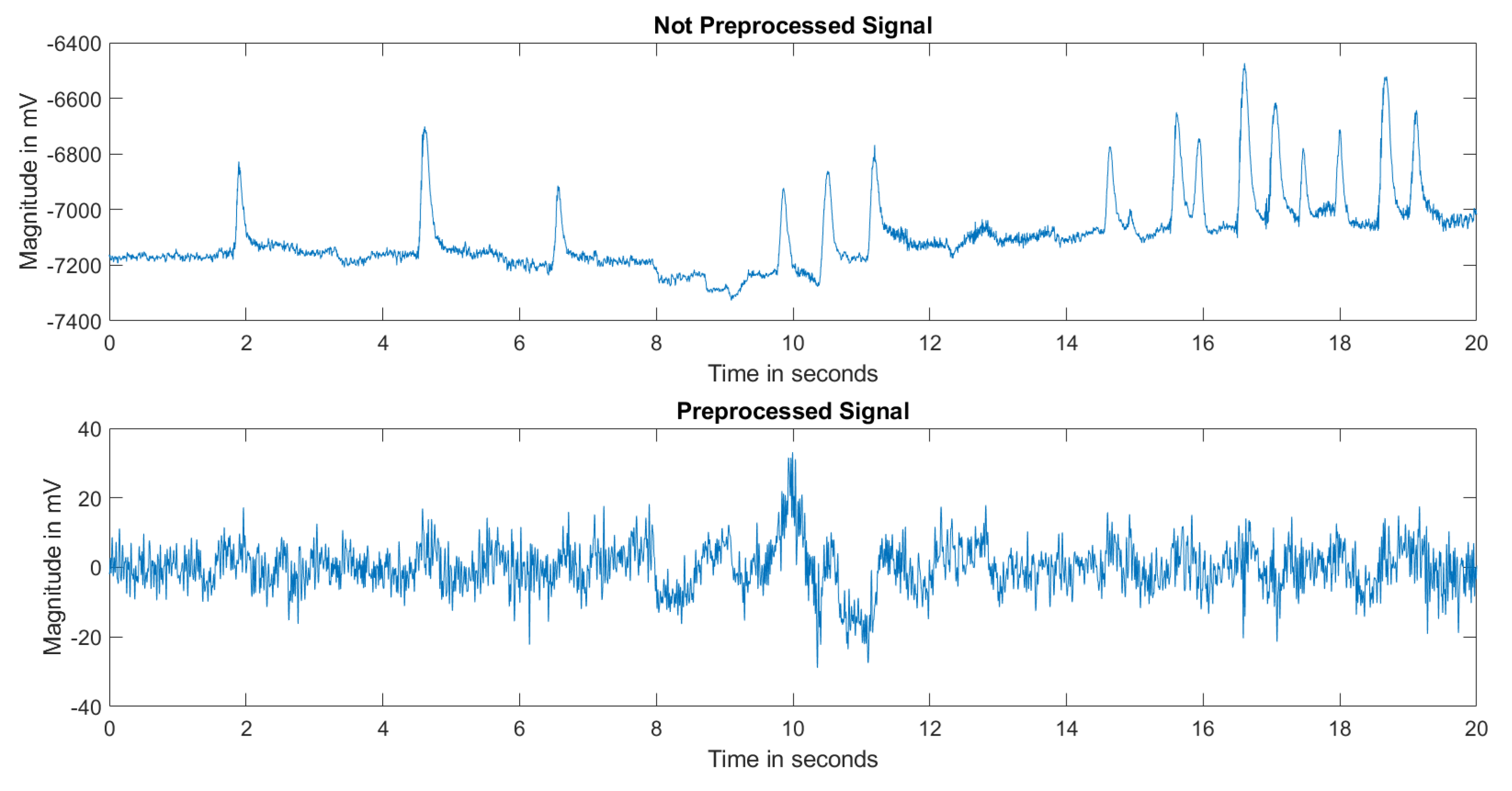
2.2. Preprocessing
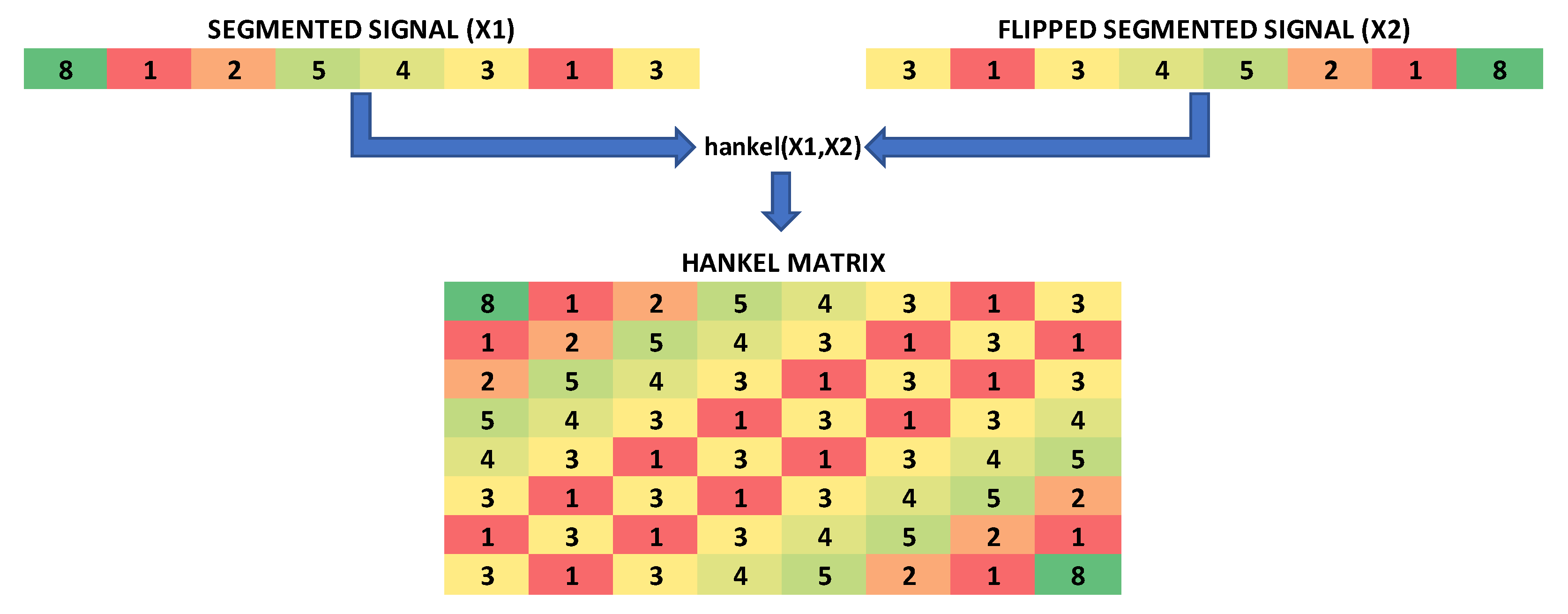
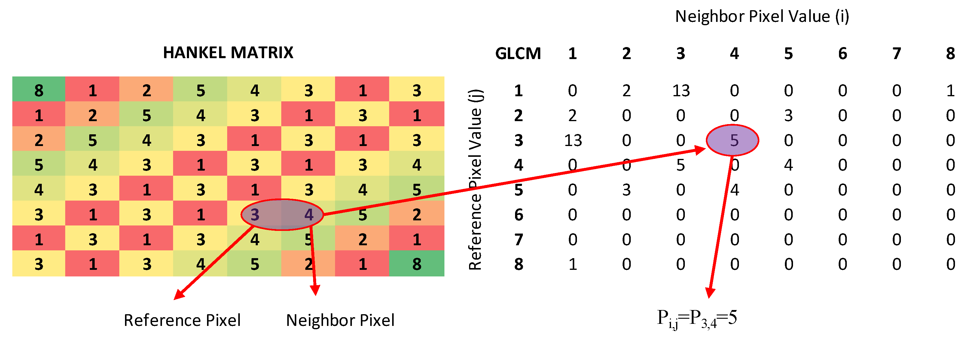
2.3. Feature Extraction and Selection
2.4. Classification
2.4.1. Feed-Forward Network
2.4.2. Support Vector Machine
2.4.3. K-Nearest Neighbor
2.4.4. Cross-Validation
2.4.5. Leave One out Cross-Validation
2.5. Performance Parameters
3. Results
4. Discussion
Supplementary Materials
Author Contributions
Funding
Institutional Review Board Statement
Informed Consent Statement
Data Availability Statement
Conflicts of Interest
References
- Donaldson, I.M. James Parkinson’s essay on the shaking palsy. J. R. Coll. Physicians Edinb. 2015, 45, 84–86. [Google Scholar] [CrossRef] [PubMed]
- de Lau, L.M.; Breteler, M.M. Epidemiology of Parkinson’s disease. Lancet Neurol. 2006, 5, 525–535. [Google Scholar] [CrossRef]
- Telarović, S. Epidemiology of Parkinson’s Disease. Arch. Psychiatry Res. 2023, 59, 147–148. [Google Scholar] [CrossRef]
- World Health Organization. Parkinson Disease. Available online: https://www.who.int/news-room/fact-sheets/detail/parkinson-disease (accessed on 5 March 2023).
- Parkinson’s Foundation. Understanding Parkinson’s Statistics. Available online: https://www.parkinson.org/understanding-parkinsons/statistics (accessed on 5 March 2023).
- Li, K.; Ao, B.; Wu, X.; Wen, Q.; Ul Haq, E.; Yin, J. Parkinson’s disease detection and classification using EEG based on deep CNN-LSTM model. Biotechnol. Genet. Eng. Rev. 2023, 1–20. [Google Scholar] [CrossRef] [PubMed]
- Akbayır, E.; Şen, M.; Ay, U.; Şenyer, S.; Tüzün, E.; Küçükali, C.İ. Parkinson Hastalığının Etyopatogenezi. Deney. Tip Derg. 2017, 7, 1–23. [Google Scholar]
- Rizzo, G.; Copetti, M.; Arcuti, S.; Martino, D.; Fontana, A.; Logroscino, G. Accuracy of clinical diagnosis of Parkinson disease: A systematic review and meta-analysis. Neurology 2016, 86, 566–576. [Google Scholar] [CrossRef]
- Qiu, L.; Li, J.; Pan, J. Parkinson’s disease detection based on multi-pattern analysis and multi-scale convolutional neural networks. Front. Neurosci. 2022, 16, 957181. [Google Scholar] [CrossRef]
- Kingdom, Parkinson’s Disease Society of the United. Types of Parkinsonism. Available online: https://www.parkinsons.org.uk/information-and-support/types-parkinsonism (accessed on 4 April 2023).
- Feraco, P.; Gagliardo, C.; La Tona, G.; Bruno, E.; D’Angelo, C.; Marrale, M.; Del Poggio, A.; Malaguti, M.C.; Geraci, L.; Baschi, R.; et al. Imaging of Substantia Nigra in Parkinson’s Disease: A Narrative Review. Brain Sci. 2021, 11, 769. [Google Scholar] [CrossRef]
- Brooks, D.J. Imaging approaches to Parkinson disease. J. Nucl. Med. 2010, 51, 596–609. [Google Scholar] [CrossRef]
- Tolosa, E.; Wenning, G.; Poewe, W. The diagnosis of Parkinson’s disease. Lancet Neurol. 2006, 5, 75–86. [Google Scholar] [CrossRef]
- Oueslati, A. Implication of Alpha-Synuclein Phosphorylation at S129 in Synucleinopathies: What Have We Learned in the Last Decade? J. Park. Dis. 2016, 6, 39–51. [Google Scholar] [CrossRef]
- Anjum, M.F.; Dasgupta, S.; Mudumbai, R.; Singh, A.; Cavanagh, J.F.; Narayanan, N.S. Linear predictive coding distinguishes spectral EEG features of Parkinson’s disease. Park. Relat. Disord. 2020, 79, 79–85. [Google Scholar] [CrossRef] [PubMed]
- Ananthi, A.; Subathra, M.S.P.; George, S.T.; Prasanna, J. A review on-EEG signals by motor imagery based brain computer interface. AIP Conf. Proc. 2022, 2670, 020010. [Google Scholar] [CrossRef]
- Tinkhauser, G.; Pogosyan, A.; Tan, H.; Herz, D.M.; Kuhn, A.A.; Brown, P. Beta burst dynamics in Parkinson’s disease OFF and ON dopaminergic medication. Brain 2017, 140, 2968–2981. [Google Scholar] [CrossRef] [PubMed]
- Maitín, A.M.; García-Tejedor, A.J.; Muñoz, J.P.R. Machine Learning Approaches for Detecting Parkinson’s Disease from EEG Analysis: A Systematic Review. Appl. Sci. 2020, 10, 8662. [Google Scholar] [CrossRef]
- Wang, Q.; Meng, L.; Pang, J.; Zhu, X.; Ming, D. Characterization of EEG Data Revealing Relationships with Cognitive and Motor Symptoms in Parkinson’s Disease: A Systematic Review. Front. Aging Neurosci. 2020, 12, 587396. [Google Scholar] [CrossRef]
- Maitin, A.M.; Romero Muñoz, J.P.; García-Tejedor, Á.J. Survey of Machine Learning Techniques in the Analysis of EEG Signals for Parkinson’s Disease: A Systematic Review. Appl. Sci. 2022, 12, 6967. [Google Scholar] [CrossRef]
- Haralick, R.M.; Shanmugam, K.; Dinstein, I.H. Textural features for image classification. IEEE Trans. Syst. Man Cybern. 1973, SMC-3, 610–621. [Google Scholar] [CrossRef]
- Gantmacher, F.R.; Brenner, J.L. Applications of the Theory of Matrices; Courier Corporation, Dover Publications Inc.: Mineola, NY, USA, 2005. [Google Scholar]
- Cavanagh, J.F.; Napolitano, A.; Wu, C.; Mueen, A. The Patient Repository for EEG Data + Computational Tools (PRED + CT). Front. Neuroinform. 2017, 11, 67. [Google Scholar] [CrossRef]
- Railo, H.; Suuronen, I.; Kaasinen, V.; Murtojärvi, M.; Pahikkala, T.; Airola, A. Resting state EEG as a biomarker of Parkinson’s disease: Influence of measurement conditions. bioRxiv 2020. [Google Scholar] [CrossRef]
- Delorme, A.; Makeig, S. EEGLAB: An open source toolbox for analysis of single-trial EEG dynamics including independent component analysis. J. Neurosci. Methods 2004, 134, 9–21. [Google Scholar] [CrossRef]
- Makeig, S.; Debener, S.; Onton, J.; Delorme, A. Mining event-related brain dynamics. Trends Cogn. Sci. 2004, 8, 204–210. [Google Scholar] [CrossRef]
- Haralick, R.M.; Shapiro, L.G. Computer and Robot Vision; Addison-Wesley Reading: Boston, MA, USA, 1992; Volume 1. [Google Scholar]
- Soh, L.-K.; Tsatsoulis, C. Texture analysis of SAR sea ice imagery using gray level co-occurrence matrices. IEEE Trans. Geosci. Remote Sens. 1999, 37, 780–795. [Google Scholar] [CrossRef]
- Clausi, D.A. An analysis of co-occurrence texture statistics as a function of grey level quantization. Can. J. Remote Sens. 2002, 28, 45–62. [Google Scholar] [CrossRef]
- Lofstedt, T.; Brynolfsson, P.; Asklund, T.; Nyholm, T.; Garpebring, A. Gray-level invariant Haralick texture features. PLoS ONE 2019, 14, e0212110. [Google Scholar] [CrossRef] [PubMed]
- Glcmfeatures(Glcm) 2.1.1.0, Version 2.1.1.0; MATLAB Central File Exchange. Available online: https://www.mathworks.com/matlabcentral/fileexchange/55034-glcmfeatures-glcm (accessed on 4 March 2023).
- Onwuegbuche, F.C.; Jurcut, D.A.; Pasquale, L. Enhancing Ransomware Classification with Multi-Stage Feature Selection and Data Imbalance Correction. In Proceedings of the 7th International Symposium on Security, Cryptography and Machine Learning, Be’er Sheva, Israel, 29–30 June 2023. [Google Scholar]
- Liu, H.; Setiono, R. Chi2: Feature Selection and Discretization of Numeric Attributes. In Proceedings of the 7th IEEE International Conference on Tools with Artificial Intelligence, Herndon, VA, USA, 5–8 November 1995. [Google Scholar]
- Krogh, A. What are artificial neural networks? Nat. Biotechnol. 2008, 26, 195–197. [Google Scholar] [CrossRef]
- Avuçlu, E. Determining the most accurate machine learning algorithms for medical diagnosis using the monk’problems database and statistical measurements. J. Exp. Theor. Artif. Intell. 2023, 1–20. [Google Scholar] [CrossRef]
- Istiadi, I.; Rahman, A.Y.; Wisnu, A.D.R. Identification of Tempe Fermentation Maturity Using Principal Component Analysis and K-Nearest Neighbor. Sink. J. Dan Penelit. Tek. Inform. 2023, 8, 286–294. [Google Scholar] [CrossRef]
- Chen, D.; Song, Q.; Zhang, Y.; Li, L.; Yang, Z. Identification of Network Traffic Intrusion Using Decision Tree. J. Sens. 2023, 2023, 5997304. [Google Scholar] [CrossRef]
- Refaeilzadeh, P.; Tang, L.; Liu, H. Cross-validation. Encycl. Database Syst. 2009, 5, 532–538. [Google Scholar]
- Shah, D.; Gopika, G.K.; Sinha, N. Analysis of EEG for Parkinson’s Disease Detection. In Proceedings of the 2022 IEEE International Conference on Signal Processing and Communications (SPCOM), Bangalore, India, 11–15 July 2022; pp. 1–5. [Google Scholar]
- Kurbatskaya, A.; Jaramillo-Jimenez, A.; Ochoa-Gomez, J.F.; Brønnick, K.; Fernandez-Quilez, A. Machine Learning-Based Detection of Parkinson’s Disease From Resting-State EEG: A Multi-Center Study. arXiv 2023, arXiv:2303.01389. [Google Scholar]
- Suuronen, I.; Airola, A.; Pahikkala, T.; Murtojarvi, M.; Kaasinen, V.; Railo, H. Budget-based classification of Parkinson’s disease from resting state EEG. IEEE J. Biomed. Health Inform. 2023, 1–9. [Google Scholar] [CrossRef] [PubMed]
- Chaturvedi, M.; Hatz, F.; Gschwandtner, U.; Bogaarts, J.G.; Meyer, A.; Fuhr, P.; Roth, V. Quantitative EEG (QEEG) Measures Differentiate Parkinson’s Disease (PD) Patients from Healthy Controls (HC). Front. Aging Neurosci. 2017, 9, 3. [Google Scholar] [CrossRef] [PubMed]
- Sugden, R.; Diamandis, P. Generalizable electroencephalographic classification of Parkinson’s Disease using deep learning. medRxiv 2022. [Google Scholar] [CrossRef]
- Shabanpour, M.; Kaboodvand, N.; Iravani, B. Parkinson’s disease is characterized by sub-second resting-state spatio-oscillatory patterns: A contribution from deep convolutional neural network. Neuroimage Clin. 2022, 36, 103266. [Google Scholar] [CrossRef] [PubMed]
- Vanneste, S.; Song, J.J.; De Ridder, D. Thalamocortical dysrhythmia detected by machine learning. Nat. Commun. 2018, 9, 1103. [Google Scholar] [CrossRef]
- Yuvaraj, R.; Acharya, U.R.; Hagiwara, Y. A novel Parkinson’s Disease Diagnosis Index using higher-order spectra features in EEG signals. Neural Comput. Appl. 2016, 30, 1225–1235. [Google Scholar] [CrossRef]
- Lee, S.B.; Kim, Y.J.; Hwang, S.; Son, H.; Lee, S.K.; Park, K.I.; Kim, Y.G. Predicting Parkinson’s disease using gradient boosting decision tree models with electroencephalography signals. Park. Relat. Disord. 2022, 95, 77–85. [Google Scholar] [CrossRef]
- Aljalal, M.; Aldosari, S.A.; Molinas, M.; AlSharabi, K.; Alturki, F.A. Detection of Parkinson’s disease from EEG signals using discrete wavelet transform, different entropy measures, and machine learning techniques. Sci. Rep. 2022, 12, 22547. [Google Scholar] [CrossRef]
- Avvaru, S.; Parhi, K.K. Effective Brain Connectivity Extraction by Frequency-Domain Convergent Cross-Mapping (FDCCM) and its Application in Parkinson’s Disease Classification. IEEE Trans. Biomed. Eng. 2023, 1–11. [Google Scholar] [CrossRef]
- Lee, S.; Hussein, R.; Ward, R.; Jane Wang, Z.; McKeown, M.J. A convolutional-recurrent neural network approach to resting-state EEG classification in Parkinson’s disease. J. Neurosci. Methods 2021, 361, 109282. [Google Scholar] [CrossRef] [PubMed]
- Aljalal, M.; Aldosari, S.A.; AlSharabi, K.; Abdurraqeeb, A.M.; Alturki, F.A. Parkinson’s Disease Detection from Resting-State EEG Signals Using Common Spatial Pattern, Entropy, and Machine Learning Techniques. Diagnostics 2022, 12, 1033. [Google Scholar] [CrossRef] [PubMed]


| Data Source | Dataset | Eyes Condition | Drug Condition |
|---|---|---|---|
| UNM | UNM_ALL | Open/Closed | On |
| UNM_OPEN | Open | On | |
| UNM_CLOSED | Closed | On | |
| UNM_OFF | Open/Closed | Off | |
| UI | UI | Open/Closed | On |
| UT | UT_OPEN | Open | Off |
| UT_CLOSED | Closed | Off |
| (Mean ± STD) | UNM | UI | UT | |||
|---|---|---|---|---|---|---|
| Condition | PD | Control | PD | Control | PD | Control |
| Sex | 17 M/10 F | 17 M/10 F | 6 M/8 F | 6 M/8 F | 9 M/11 F | 8 M/12 F |
| Age | 69.5 ± 8.7 | 69.5 ± 9.3 | 70.5 ± 8.7 | 70.5 ± 8.7 | 69.8 ± 7.2 | 67.8 ± 6.2 |
| MMSE | 28.7 ± 1 | 28.8 ± 1 | - | - | 27.8 ± 1.8 | 28.2 ± 1.5 |
| MOCA | - | - | 25.9 ± 2.7 | 27.2 ± 1.7 | - | - |
| UPDRS | 22.2 ± 10.3 | - | 13.4 ± 6.6 | - | 28.9 ± 16.4 | 5.1 ± 3.5 |
| Years from Diagnosis | 5.7 ± 4.2 | - | 5.6 ± 3.2 | - | 6.4(4.9) | - |
| Recording Minute | 3.59 ± 1 | 3.63 ± 1.8 | 3.11 ± 1.2 | 3.17 ± 0.9 | 2.55 ± 0.06 | 2.51 ± 0.2 |
| BDI | 7.6 ± 5.3 | 4.8 ± 4.8 | - | - | 8.4 ± 6.2 | 5.0 ± 3.0 |
| LED | 707.4 ± 448.6 | - | 796 ± 409 | - | 663.2 ± 509.1 | - |
| NAART | 45.2 ± 10.3 | 47.1 ± 7.5 | - | - | - | - |
| FF | SVM | KNN |
|---|---|---|
| Layer Size = [10] Activation Function = Relu | Kernel Function = Linear Kernel Scale = 1 Box Constraint = 1 | 1 Neighbor Euclidean Distance |
| AUC | ACC | SENS | SPEC | PPV | NPV | |
|---|---|---|---|---|---|---|
| UNM_All | 92.84 | 92.41 | 92.96 | 91.85 | 91.96 | 92.96 |
| (91.08–94.24) | (90.74–94.44) | (88.89–96.3) | (88.89–92.59) | (89.29–92.86) | (89.29–96.15) | |
| UNM_Closed | 94.44 | 89.07 | 90 | 88.15 | 88.38 | 89.84 |
| (92.18–95.47) | (87.04–90.74) | (88.89–92.59) | (85.19–88.89) | (85.71–89.29) | (88.46–92.31) | |
| UNM_Open | 94.9 | 89.44 | 89.63 | 89.26 | 89.46 | 89.66 |
| (92.87–95.61) | (87.04–94.44) | (85.19–92.59) | (85.19–96.3) | (85.71–96.15) | (85.71–92.86) | |
| UNM_Off | 90.66 | 83.89 | 88.15 | 79.63 | 81.34 | 87.16 |
| (87.93–92.46) | (79.63–87.04) | (81.48–92.59) | (70.37–85.19) | (75.76–85.71) | (80.77–91.67) | |
| UI | 87.4 | 85.71 | 94.29 | 77.14 | 80.5 | 93.31 |
| (82.14–89.8) | (82.14–89.29) | (85.71–100) | (71.43–78.57) | (76.47–82.35) | (84.62–100) | |
| UT_Closed | 84 | 77.18 | 73 | 81.58 | 80.86 | 74.45 |
| (77.37–88.95) | (66.67–84.62) | (60–85) | (68.42–89.47) | (70–88.89) | (63.64–84.21) | |
| UT_Open | 67.85 | 63.25 | 77 | 49.5 | 60.49 | 68.26 |
| (64.75–71.25) | (60–67.5) | (70–80) | (40–55) | (57.14–64) | (62.5–73.33) |
| AUC | ACC | SENS | SPEC | PPV | NPV | |
|---|---|---|---|---|---|---|
| UNM_All | 94.39 | 93.7 | 93.22 | 94.16 | 94.16 | 93.51 |
| (87.72–100) | (90.74–98.15) | (88–100) | (88.89–100) | (88.46–100) | (88.46–100) | |
| UNM_Closed | 94.11 | 89.26 | 92.22 | 86.23 | 87.26 | 91.68 |
| (89.71–96.98) | (83.33–92.59) | (88–96.15) | (74.07–96) | (78.13–96.3) | (88.89–96.67) | |
| UNM_Open | 94.55 | 87.04 | 86.23 | 87.76 | 86.88 | 87.23 |
| (90.67–98.32) | (77.78–92.59) | (72–96.3) | (81.25–95.83) | (72.73–96.43) | (78.79–96) | |
| UNM_Off | 91.07 | 83.33 | 87.99 | 78.53 | 80.45 | 87.29 |
| (83.68–95.45) | (72.22–88.89) | (74.07–96.3) | (70.37–90.63) | (71.43–88.89) | (73.08–95) | |
| UI | 85.21 | 82.5 | 88.9 | 75.35 | 79.42 | 85.82 |
| (78.06–96.11) | (75–92.86) | (78.57–100) | (57.14–94.44) | (66.67–93.75) | (71.43–100) | |
| UT_Closed | 83.21 | 76.92 | 73.97 | 80.65 | 80.57 | 73.07 |
| (72.86–91.3) | (66.67–84.62) | (64–85.71) | (70–93.75) | (66.67–94.12) | (52.63–90.48) | |
| UT_Open | 61.93 | 59.75 | 78.61 | 41.53 | 55.29 | 68.31 |
| (39.64–80.3) | (45–75) | (47.06–89.47) | (23.53–68.18) | (38.1–68.18) | (50–83.33) |
| UNM_All | UI | UT_Closed | |||
|---|---|---|---|---|---|
| Shah et al. [39] | 88.5 | Qiu et al. [9] | 96.31 | Kurbatskaya et al. [40] | 82.2 |
| Anjum et al. [15] | 85.2 | Anjum et al. [15] | 85.7 | Suuronen et al. [41] | 76 |
| Chaturverdi et al. [42] | 72.2 | Sugden et al. [43] | 83.8 | Shabanpour et al. [44] | 63.44 |
| Vanneste et al. [45] | 72.2 | Proposed | 85.71 | Proposed | 76.92 |
| Yuvaraj et al. [46] | 59.3 | ||||
| Lee et al. [47] | 89.3 | ||||
| Sugden et al. [43] | 69.2 | ||||
| Aljalal et al. [48] | 87.04 | ||||
| Avvaru et al. [49] | 79.25 | ||||
| Proposed | 93.7 | ||||
Disclaimer/Publisher’s Note: The statements, opinions and data contained in all publications are solely those of the individual author(s) and contributor(s) and not of MDPI and/or the editor(s). MDPI and/or the editor(s) disclaim responsibility for any injury to people or property resulting from any ideas, methods, instructions or products referred to in the content. |
© 2023 by the authors. Licensee MDPI, Basel, Switzerland. This article is an open access article distributed under the terms and conditions of the Creative Commons Attribution (CC BY) license (https://creativecommons.org/licenses/by/4.0/).
Share and Cite
Karakaş, M.F.; Latifoğlu, F. Distinguishing Parkinson’s Disease with GLCM Features from the Hankelization of EEG Signals. Diagnostics 2023, 13, 1769. https://doi.org/10.3390/diagnostics13101769
Karakaş MF, Latifoğlu F. Distinguishing Parkinson’s Disease with GLCM Features from the Hankelization of EEG Signals. Diagnostics. 2023; 13(10):1769. https://doi.org/10.3390/diagnostics13101769
Chicago/Turabian StyleKarakaş, Mehmet Fatih, and Fatma Latifoğlu. 2023. "Distinguishing Parkinson’s Disease with GLCM Features from the Hankelization of EEG Signals" Diagnostics 13, no. 10: 1769. https://doi.org/10.3390/diagnostics13101769
APA StyleKarakaş, M. F., & Latifoğlu, F. (2023). Distinguishing Parkinson’s Disease with GLCM Features from the Hankelization of EEG Signals. Diagnostics, 13(10), 1769. https://doi.org/10.3390/diagnostics13101769