
Generation of Digital Brain Phantom for Machine Learning Application of Dopamine Transporter Radionuclide Imaging

 ,
,  and
and 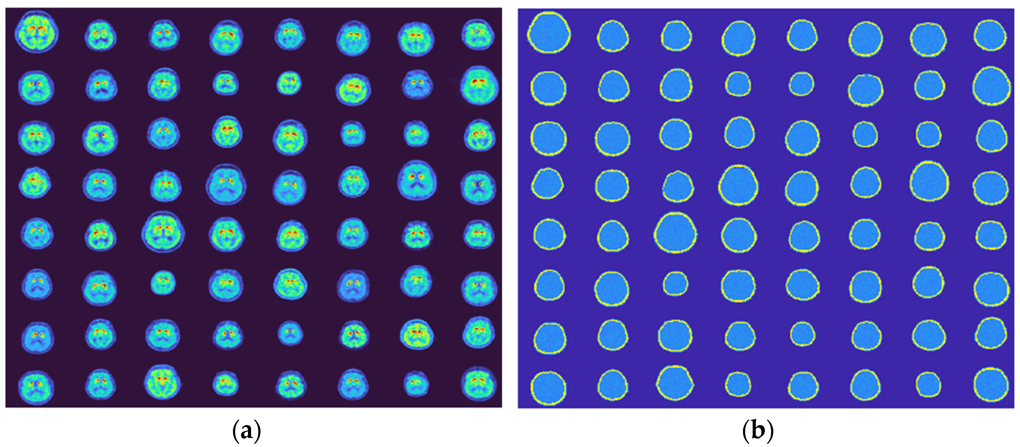
Abstract
:1. Introduction
2. Data and Methods
2.1. Training Datasets Preparation
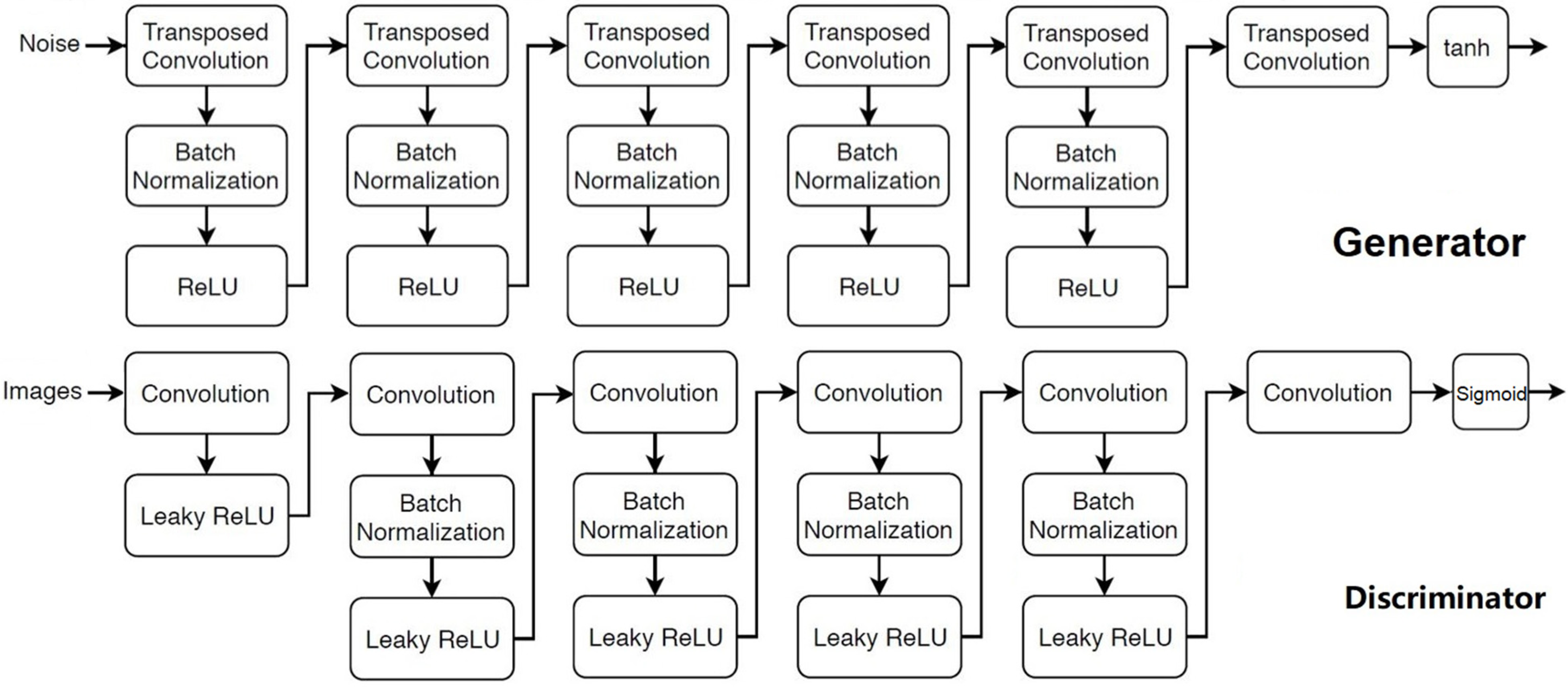
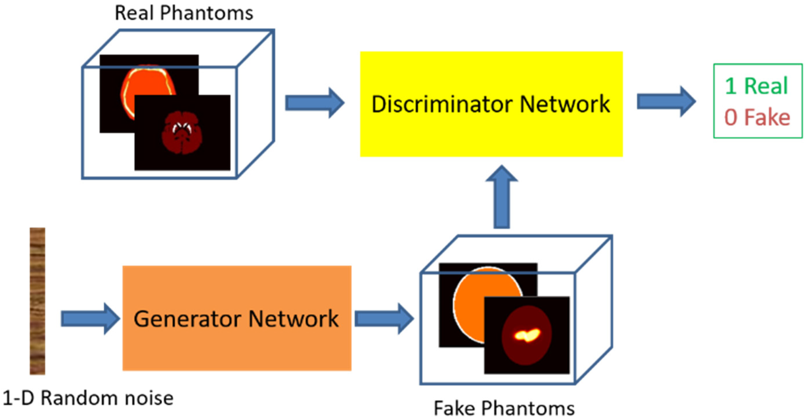
2.2. Neural Network Details and Training
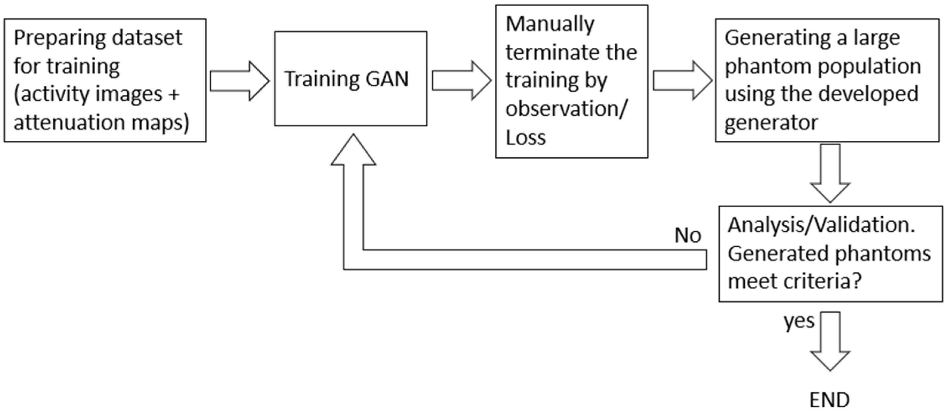
2.3. Optimization of Training
3. Results
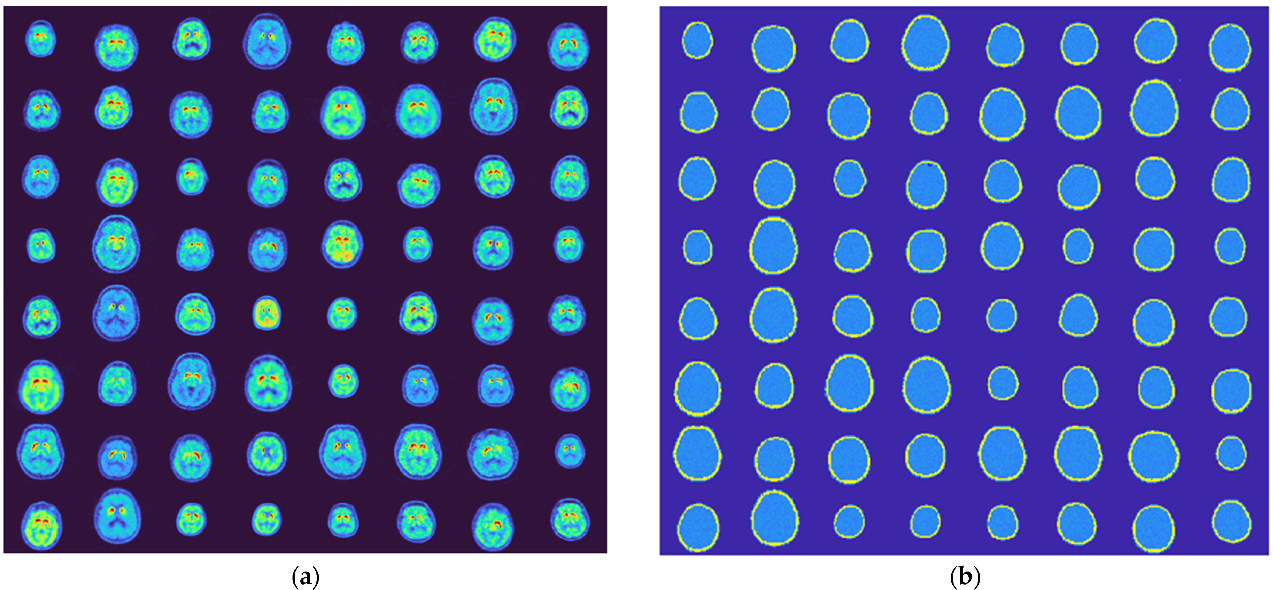
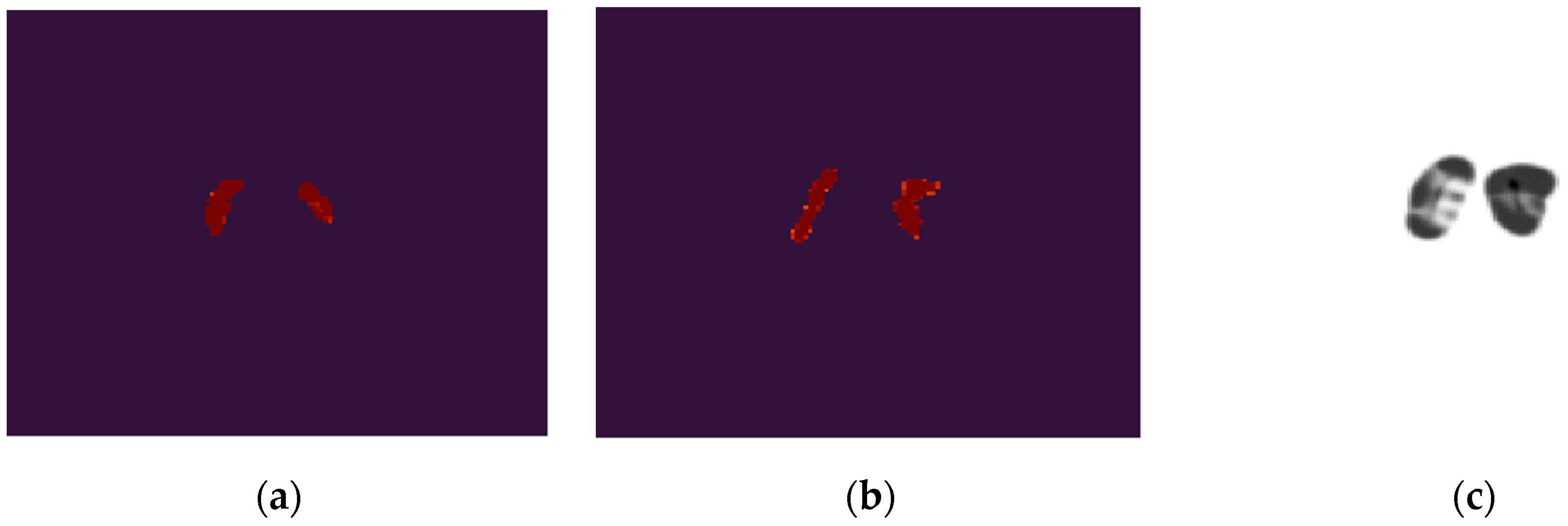
3.1. Generated Phantoms
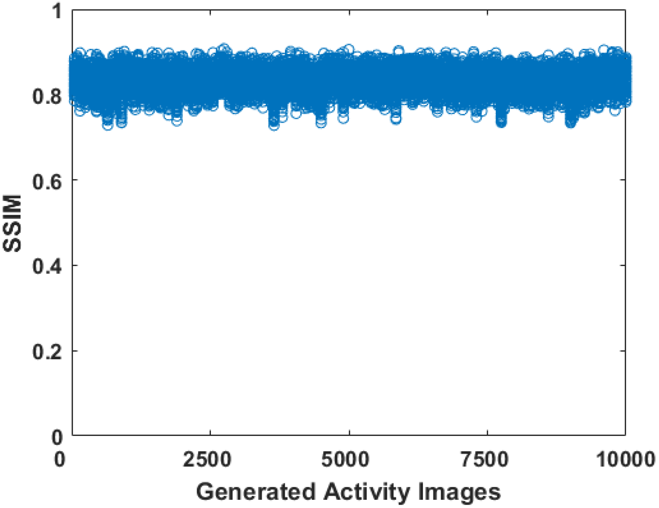
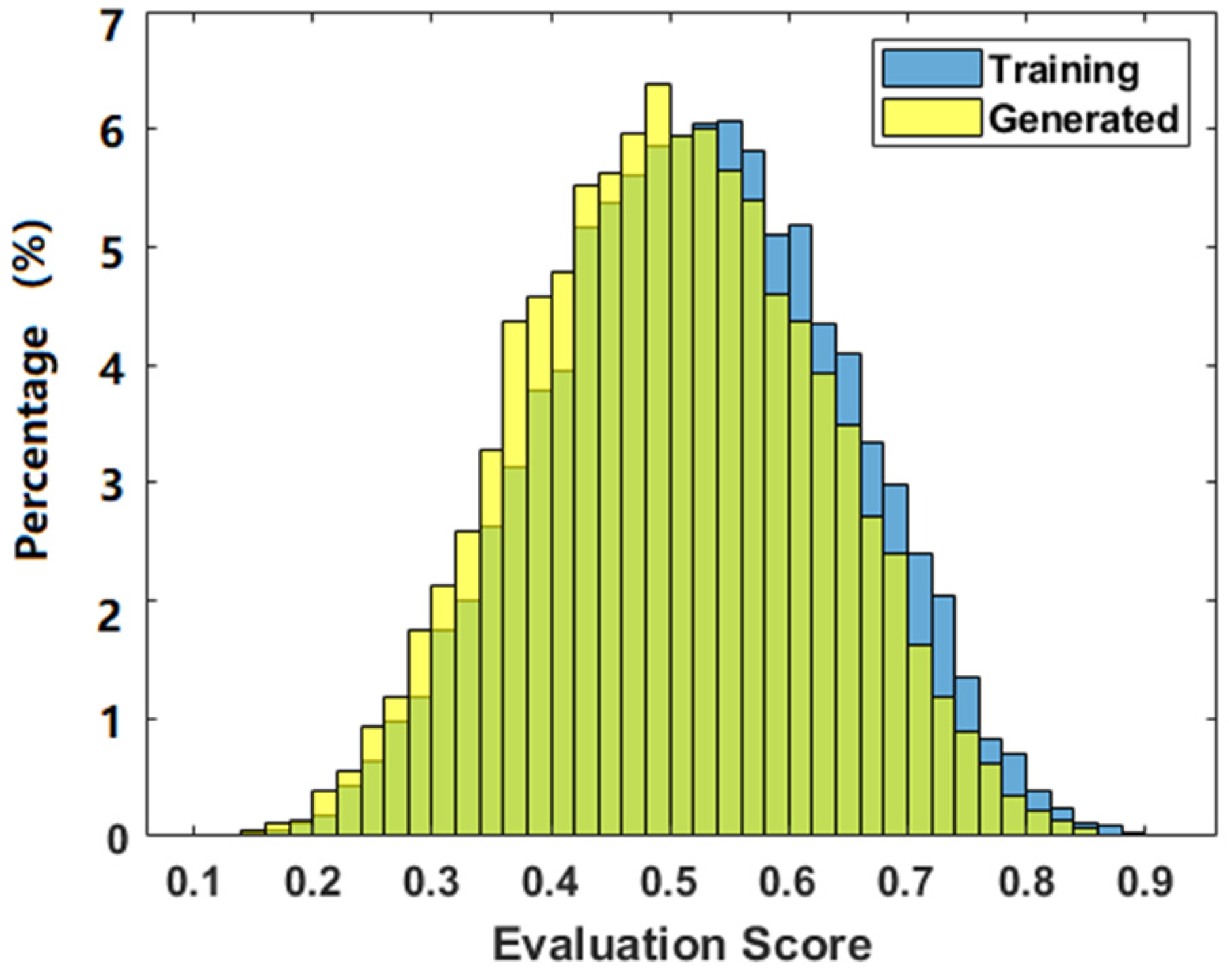
3.2. Evaluation of the Phantoms
4. Discussion
5. Conclusions
6. Patents
Author Contributions
Funding
Institutional Review Board Statement
Informed Consent Statement
Data Availability Statement
Conflicts of Interest
References
- Benamer, H.T.S.; Patterson, J.; Grosset, D.; Booij, J.; De Bruin, K.; Van Royen, E.; Speelman, J.D.; Horstink, M.H.I.M.; Sips, H.J.W.A.; Dierckx, R.A.; et al. Accurate differentiation of Parkinsonism and essential tremor using visual assessment of [I-123]-FP-CIT SPECT imaging: The [I-123]-FP-CIT study group. Mov. Disord. 2000, 15, 503–510. [Google Scholar] [CrossRef]
- Poewe, W.; Wenning, G. The differential diagnosis of Parkinson’s disease. Eur. J. Neurol. 2002, 9, 23–30. [Google Scholar] [CrossRef] [PubMed]
- Weng, Y.-H.; Yen, T.-C.; Chen, M.-C.; Kao, P.-F.; Tzen, K.-Y.; Chen, R.-S.; Wey, S.-P.; Ting, G.; Lu, C.-S. Sensitivity and specificity of Tc-99m- TRODAT-1 SPECT imaging in differentiating patients with idiopathic Parkinson’s disease from healthy subjects. J. Nucl. Med. 2004, 45, 393–401. [Google Scholar] [PubMed]
- Schindler, T.H.; Rschelbert, H.R.; Quercioli, A.; Dilsizian, V. Cardiac PET imaging for the detection and monitoring of coronary artery disease and microvascular health. JACC Cardiovasc. Imaging 2010, 3, 623–640. [Google Scholar] [CrossRef]
- Abbott, B.G.; Case, J.A.; Dorbala, S.; Einstein, A.J.; Galt, J.R.; Pagnanelli, R.; Bullock-Palmer, R.P.; Soman, P.; Wells, G.R. Contemporary cardiac SPECT imaging—Innovations and best practices: An information statement from the American Society of Nuclear Cardiology. J. Nucl. Cardiol. 2018, 25, 1847–1860. [Google Scholar] [CrossRef]
- Van Dort, M.E.; Rehemtulla, A.; Ross, B.D. PET and SPECT imaging of tumor biology: New approaches towards oncology drug discovery and development. Curr. Comput. Aided Drug Des. 2008, 4, 46–53. [Google Scholar] [CrossRef]
- Kennedy, J.A.; Israel, O.; Frenkel, A.; Bar-Shalom, R.; Azhai, H. Super-resolution in PET imaging. IEEE Trans. Med. Imaging 2006, 25, 137–147. [Google Scholar] [CrossRef]
- Khalil, M.M.; Tremoleda, J.L.; Bayomy, T.B.; Gswll, W. Molecular SPECT imaging: An overview. Inter. J. Mol. Imaging 2011, 2011, 796025. [Google Scholar] [CrossRef]
- Zhu, B.; Liu, J.Z.; Cauley, S.F.; Rosen, B.R.; Rosen, M.S. Image reconstruction by domain-transform manifold learning. Nature 2018, 555, 487–495. [Google Scholar] [CrossRef]
- Yang, G.; Yu, S.; Dong, H.; Slabaugh, G.; Dragotti, P.L.; Ye, X.; Liu, F.; Arridge, S.; Keegan, J.; Guo, Y.; et al. DAGAN: Deep de-aliasing generative adversarial networks for fast compressed sensing MRI reconstruction. IEEE Trans. Med. Imaging 2018, 37, 1310–1321. [Google Scholar] [CrossRef]
- Quan, T.M.; Nguyen-duc, T.; Jeong, W. Compressed sensing MRI reconstruction using a generative adversarial network with a cyclic loss. IEEE Trans. Med. Imaging 2018, 37, 1488–1497. [Google Scholar] [CrossRef] [PubMed]
- Han, Y.; Ye, J.C. Framing U-net via deep convolutional framelets: Application to sparse-view CT. IEEE Trans. Med. Imaging 2018, 37, 1418–1429. [Google Scholar] [CrossRef] [PubMed]
- Chen, H.; Zhang, Y.; Chen, Y.; Zhang, J.; Zhang, W.; Sun, H.; Lv, Y.; Liao, P.; Zhou, J.; Wang, G. LEARN: Learned experts’ assessment-based reconstruction network for sparse-data CT. IEEE Trans. Med. Imaging 2018, 37, 1333–1347. [Google Scholar] [CrossRef] [PubMed]
- Gupta, H.; Jin, K.H.; Nguyen, H.Q.; McCann, M.T.; Unser, M. CNN-based projected gradient descent for consistent CT image reconstruction. IEEE Trans. Med. Imaging 2018, 37, 1440–1453. [Google Scholar] [CrossRef] [PubMed]
- Kim, K.; Wu, D.; Gong, K.; Dutta, J.; Kim, J.H.; Son, Y.D.; Kim, H.K.; El Fakhri, G.; Li, Q. Penalized PET reconstruction using deep learning prior and local linear fitting. IEEE Trans. Med. Imaging 2018, 37, 1478–1487. [Google Scholar] [CrossRef]
- Hwang, D.; Kim, K.Y.; Kang, S.K.; Seo, S.; Paeng, J.C.; Lee, D.S.; Lee, J.S. Improving the accuracy of simultaneously reconstructed activity and attenuation maps using deep learning. J. Nucl. Med. 2018, 59, 1624–1629. [Google Scholar] [CrossRef] [PubMed]
- Hwang, D.; Kang, S.K.; Kim, K.Y.; Seo, S.; Paeng, J.C.; Lee, D.S.; Lee, J.S. Generation of PET attenuation map for whole-body time-of-flight 18F-FDG PET/MRI using deep neural network trained with simultaneously reconstructed activity and attenuation maps. J. Nucl. Med. 2019, 60, 1183–1189. [Google Scholar] [CrossRef]
- Gong, K.; Han, P.K.; Johnson, K.A.; Fakhri, G.; Ma, C.; Li, Q. Attenuation correction using deep learning and integrated UTE/multi-echo Dixon sequence: Evaluation in amyloid and tau PET imaging. Eur. J. Nucl. Med. Mol. Imaging 2020, 48, 1351–1361. [Google Scholar] [CrossRef]
- Shi, L.; Onofrey, J.A.; Liu, H.; Liu, Y.H.; Liu, C. Deep learning-based attenuation map generation for myocardial perfusion SPECT. Eur. J. Nucl. Med. Mol. Imaging 2020, 47, 2383–2395. [Google Scholar] [CrossRef]
- Shao, W.; Pomper, M.G.; Du, Y. A learned reconstruction network for SPECT imaging. IEEE Trans. Radiat. Plasma Med. Sci. 2021, 5, 26–34. [Google Scholar] [CrossRef]
- Shao, W.; Rowe, S.P.; Du, Y. SPECTnet: A deep learning neural network for SPECT image reconstruction. Ann. Trans. Med. 2021, 9, 819. [Google Scholar] [CrossRef] [PubMed]
- Shao, W.; Du, Y. SPECT image reconstruction by deep learning using a two-step training method. J. Nucl. Med. 2019, 60 (Suppl. S1), 1353. [Google Scholar]
- Du, Y.; Frey, E.C.; Wang, W.T.; Tocharoenchai, C.; Baird, W.H.; Tsui, B.M.W. Combination of MCNP and SimSET for Monte Carlo Simulation of SPECT with Medium and High Energy Photons. IEEE Trans. Nucl. Sci. 2002, 49, 668–674. [Google Scholar] [CrossRef]
- Song, X.; Segars, W.P.; Du, Y.; Tsui, B.M.W.; Frey, E.C. Fast Modeling of the Collimator-Detector Response in Monte Carlo Simulation of SPECT Imaging using the Angular Response Function. Phys. Med. Biol. 2005, 50, 1791–1804. [Google Scholar] [CrossRef] [PubMed]
- Descourt, P.; Carlier, T.; Du, Y.; Song, X.; Buvat, I.; Frey, E.C.; Bardies, M.; Tsui, B.M.W.; Visvikis, D. Implementation of angular response function modeling in SPECT simulations with GATE. Phys. Med. Biol. 2010, 55, N253–N266. [Google Scholar] [CrossRef]
- Zubal, I.G.; Harrell, C.R.; Smith, E.O.; Smith, A.L.; Krischluna, P. High resolution MRI-based, segmented, computerized head phantom. Physics 1999. Available online: https://noodle.med.yale.edu/phant.html#Zubal2 (accessed on 18 July 2022).
- Segars, W.P.; Sturgeon, G.; Mendonca, S.; Grimes, J.; Tsui, B.M.W. 4D XCAT phantom for multimodality imaging research. Med. Phys. 2010, 37, 4902–4915. [Google Scholar] [CrossRef]
- Karras, T.; Aila, T.; Laine, S.; Lehtinen, J. Progressive growing of GANs for improved quality, stability, and variation. arXiv 2018. [Google Scholar] [CrossRef]
- Leung, K.H.; Rowe, S.P.; Shao, W.; Coughlin, J.; Pomper, G.M.; Du, Y. Progressively growing GANs for realistic synthetic brain MR images. J. Nucl. Med. 2021, 62 (Suppl. S1), 1191. [Google Scholar]
- Shao, W.; Zhou, B. Dielectric breast phantoms by generative adversarial network. IEEE Trans. Antennas Propag. 2021, 1. Available online: https://jhu.pure.elsevier.com/en/publications/dielectric-breast-phantoms-by-generative-adversarial-network (accessed on 18 July 2022).
- Shao, W.; Zhou, B. Dielectric breast phantom by a conditional GAN. IEEE Proc. APS/URSI 2022, 1–3. Available online: https://2022apsursi.org/call_for_papers.php (accessed on 18 July 2022).
- Leung, K.H.; Shao, W.; Solnes, L.; Rowe, S.P.; Pomper, M.G.; Du, Y. A deep-learning based approach for disease detection in the projection space of DAT-SPECT images of patients with Parkinson’s disease. J. Nucl. Med. 2020, 61 (Suppl. S1), 509. [Google Scholar]
- Parkinson’s Progression Markers Initiative. Available online: https://www.ppmi-info.org/ (accessed on 18 July 2022).
- Kingma, D.P.; Ba, J. Adam: A method for stochastic optimization. ICLR 2015 Proc. 2015, 1–15. Available online: https://www.researchgate.net/publication/269935079_Adam_A_Method_for_Stochastic_Optimization (accessed on 18 July 2022).
- Jenni, S.; Favaro, P. On stabilizing generative adversarial training with noise. arXiv 2019. [Google Scholar] [CrossRef]
- Aronov, B.; Har-Peled, S.; Knauer, C.; Wang, Y.; Wenk, C. Fréchet distance for curves, revisited. In European Symposium on Algorithms; Lecture Notes in Computer Science 4168; Springer: Berlin/Heidelberg, Germany, 2006; pp. 52–63. [Google Scholar]
- Du, Y.; Frey, E.C.; Tsui, B.M.W. Model-based compensation for quantitative 123I brain SPECT imaging. Phys. Med. Biol. 2006, 51, 1269–1282. [Google Scholar] [CrossRef] [PubMed]
- Leung, K.H.; Salmanpour, M.R.; Saberi, A.; Klyuzhin, I.S.; Sossi, V.; Jha, A.K.; Pomper, M.G.; Du, Y. Using deep-learning to predict outcome of patients with Parkinson’s disease. In Proceedings of the 2018 IEEE Nuclear Science Symposium and Medical Imaging Conference Proceedings (NSS/MIC), Sydney, NSW, Australia, 10–17 November 2018; pp. 1–4. [Google Scholar] [CrossRef]
- Guttman, M.; Burkholder, J.; Kish, S.J.; Hussey, D.; Wilson, A.; DaSilva, J.; Houle, S. [11C]RTI-32 PET studies of the dopamine transporter in early dopa-naive Parkinson’s disease: Implications for the symptomatic threshold. Neurology 1997, 48, 1578–1583. [Google Scholar] [CrossRef] [PubMed]
- Kung, M.; Stevenson, D.A.; Plssl, K.; Meegalla, S.K.; Beckwith, A.; Essman, W.D.; Mu, M.; Lucki, I.; Kung, H. [99mTc]TRODAT-1: A novel technetium-99m complex as a dopamine transporter imaging agent. Eur. J. Nucl. Med. 1997, 24, 372–380. [Google Scholar] [CrossRef]
- Shao, W.; Leung, K.; Pomper, M.; Du, Y. SPECT image reconstruction by a learnt neural network. J. Nucl. Med. 2020, 61 (Suppl. S1), 1478. [Google Scholar]
- Shao, W.; Rowe, S.; Du, Y. Artificial intelligence in single photon emission computed tomography (SPECT) imaging: A narrative review. Ann. Trans. Med. 2021, 9, 820. [Google Scholar] [CrossRef] [PubMed]


Publisher’s Note: MDPI stays neutral with regard to jurisdictional claims in published maps and institutional affiliations. |
© 2022 by the authors. Licensee MDPI, Basel, Switzerland. This article is an open access article distributed under the terms and conditions of the Creative Commons Attribution (CC BY) license (https://creativecommons.org/licenses/by/4.0/).
Share and Cite
Shao, W.; Leung, K.H.; Xu, J.; Coughlin, J.M.; Pomper, M.G.; Du, Y. Generation of Digital Brain Phantom for Machine Learning Application of Dopamine Transporter Radionuclide Imaging. Diagnostics 2022, 12, 1945. https://doi.org/10.3390/diagnostics12081945
Shao W, Leung KH, Xu J, Coughlin JM, Pomper MG, Du Y. Generation of Digital Brain Phantom for Machine Learning Application of Dopamine Transporter Radionuclide Imaging. Diagnostics. 2022; 12(8):1945. https://doi.org/10.3390/diagnostics12081945
Chicago/Turabian StyleShao, Wenyi, Kevin H. Leung, Jingyan Xu, Jennifer M. Coughlin, Martin G. Pomper, and Yong Du. 2022. "Generation of Digital Brain Phantom for Machine Learning Application of Dopamine Transporter Radionuclide Imaging" Diagnostics 12, no. 8: 1945. https://doi.org/10.3390/diagnostics12081945
APA StyleShao, W., Leung, K. H., Xu, J., Coughlin, J. M., Pomper, M. G., & Du, Y. (2022). Generation of Digital Brain Phantom for Machine Learning Application of Dopamine Transporter Radionuclide Imaging. Diagnostics, 12(8), 1945. https://doi.org/10.3390/diagnostics12081945