
Sequential Models for Endoluminal Image Classification


Abstract
:1. Introduction
1.1. Motivation and Contribution
1.2. Related Work
2. Materials and Methods
2.1. Dataset
2.2. Outcomes
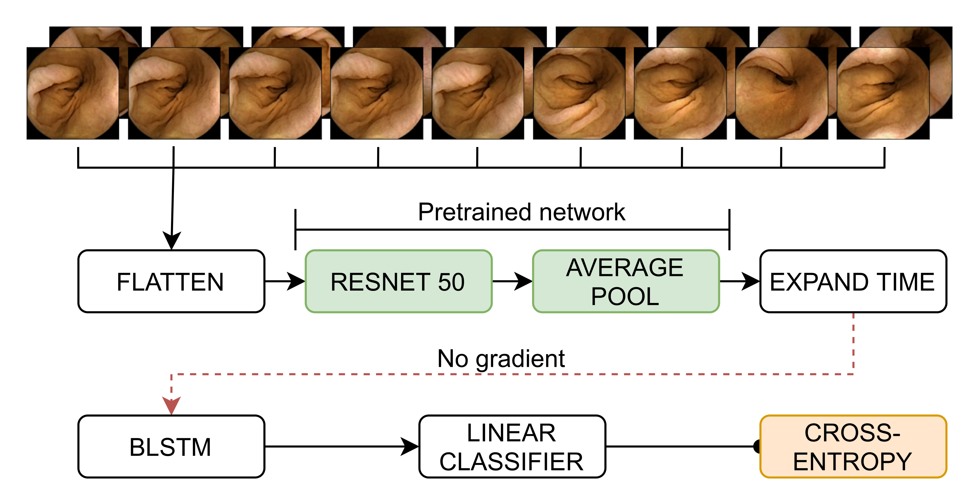
2.3. Methodology
2.4. Experiments and Evaluation
2.4.1. Implementation Details
2.4.2. Evaluation Strategies
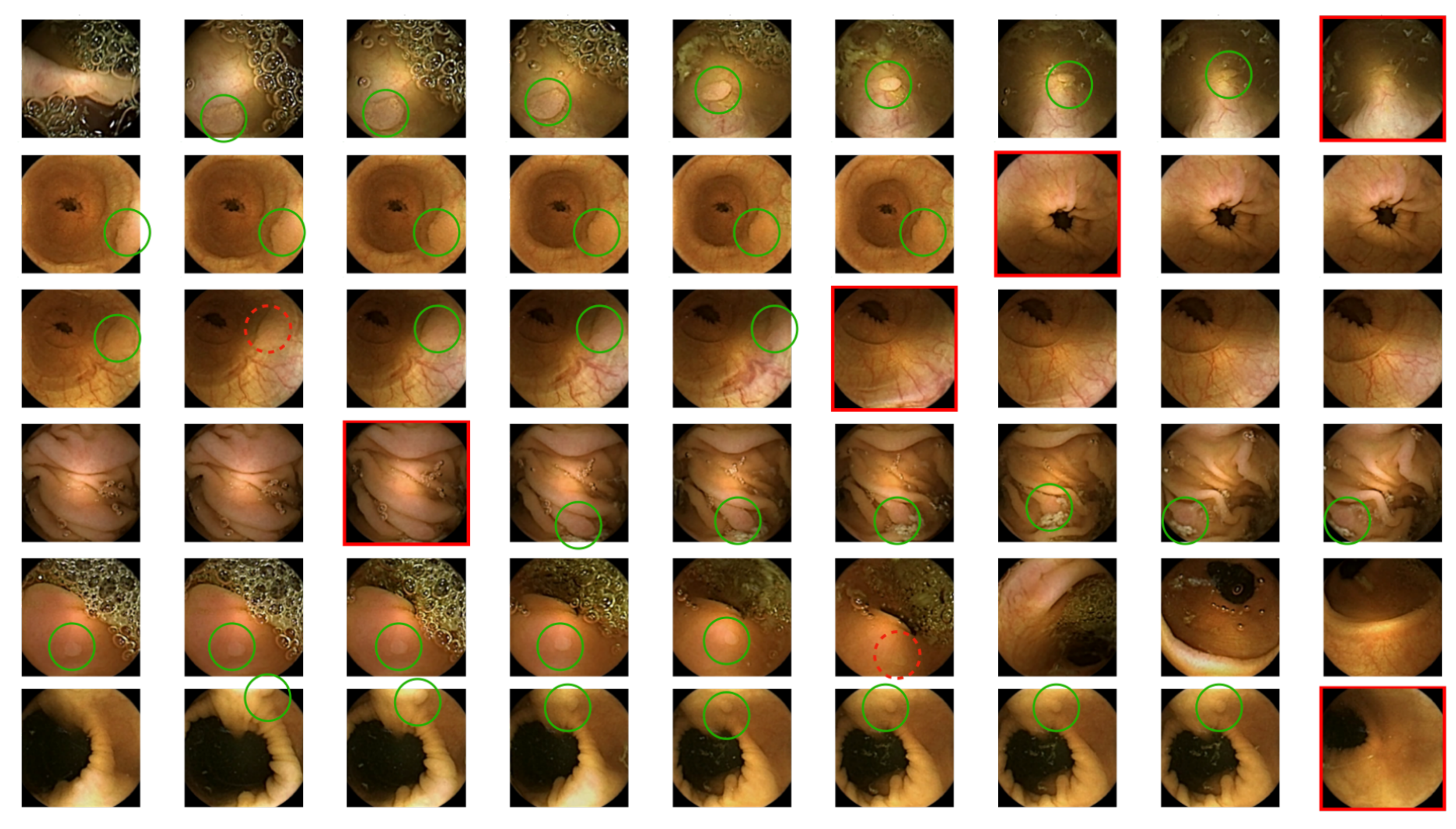
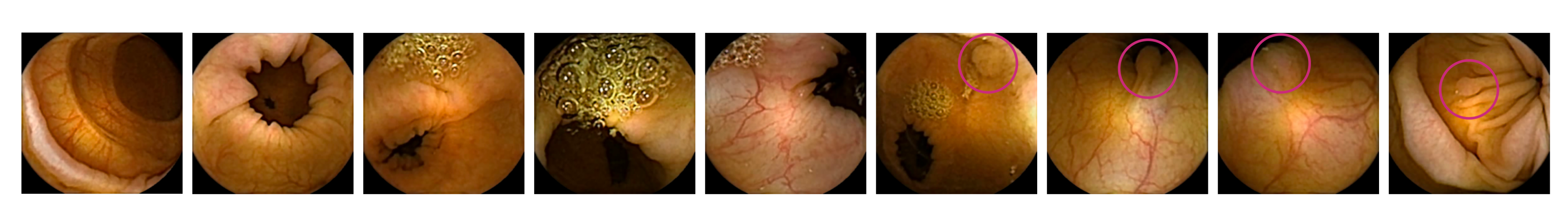
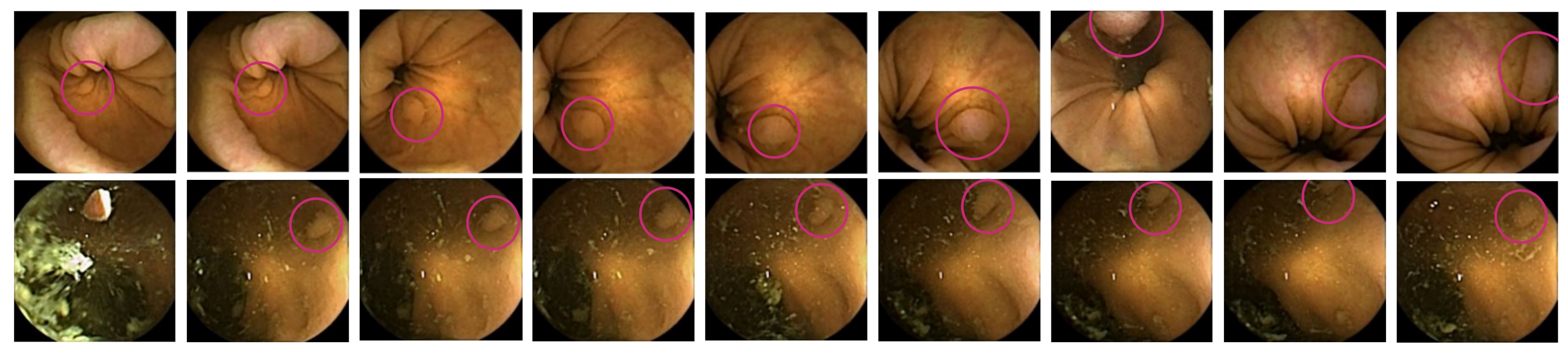
2.4.3. Qualitative Strategies
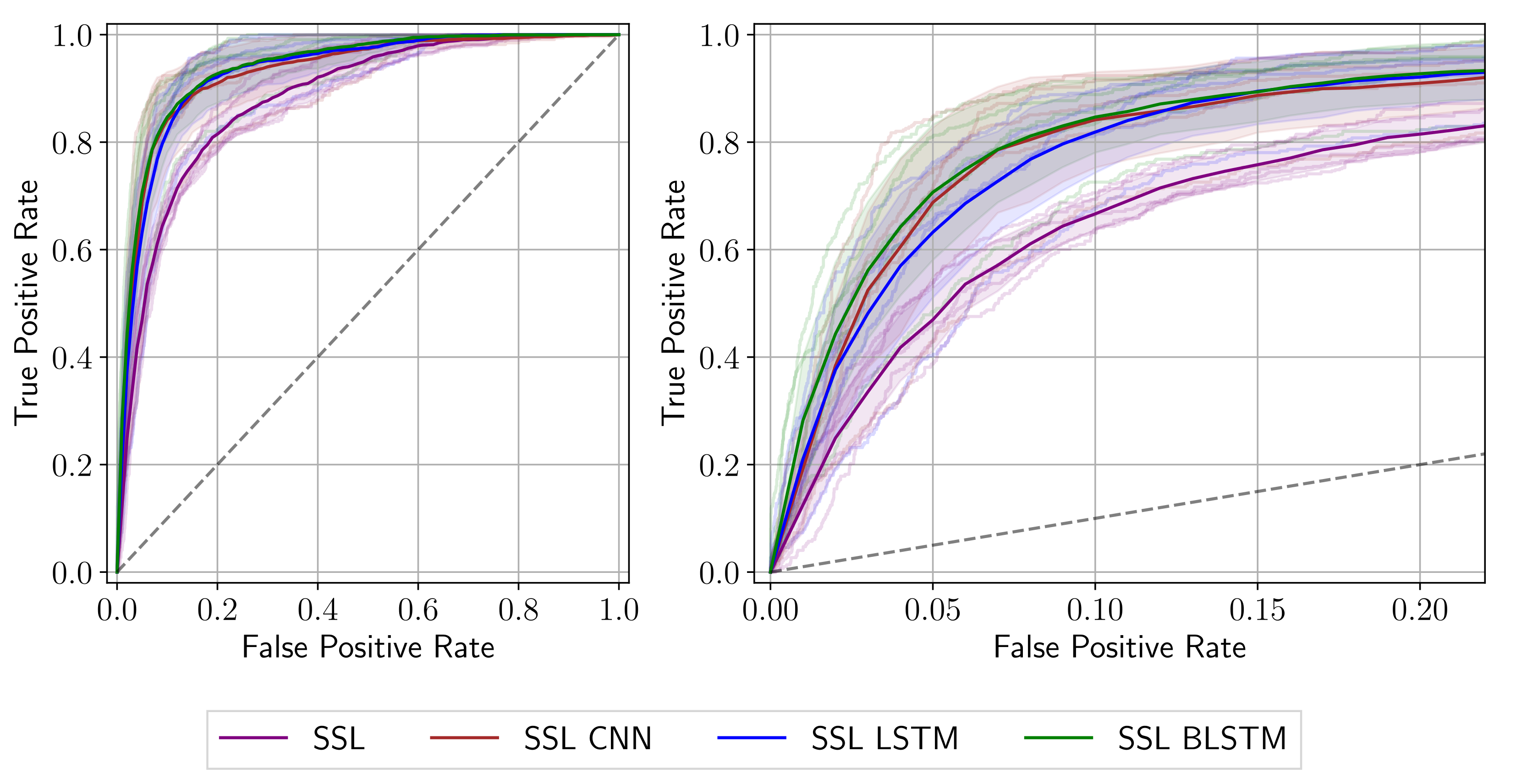
3. Results
3.1. Quantitative Results
3.2. Qualitative Results
4. Discussion
5. Conclusions
Author Contributions
Funding
Institutional Review Board Statement
Informed Consent Statement
Data Availability Statement
Acknowledgments
Conflicts of Interest
References
- Siegel, R.L.; Miller, K.D.; Jemal, A. Cancer Statistics, 2020. CA Cancer J. Clin. 2020, 70, 145–164. [Google Scholar] [CrossRef] [PubMed] [Green Version]
- Laiz, P.; Vitrià, J.; Wenzek, H.; Malagelada, C.; Azpiroz, F.; Seguí, S. WCE polyp detection with triplet based embeddings. Comput. Med. Imaging Graph. 2020, 86, 101794. [Google Scholar] [CrossRef] [PubMed]
- Swain, P.; Iddan, G.; Meron, G.; Glukhovsky, A. Wireless capsule endoscopy of the small-bowel: Development, testing and first human trials. Biomonit. Endosctechnol. 2001, 29, 19–23. [Google Scholar] [CrossRef]
- Rahim, T.; Usman, M.A.; Shin, S.Y. A survey on contemporary computer-aided tumor, polyp, and ulcer detection methods in wireless capsule endoscopy imaging. Comput. Med. Imaging Graph. 2020, 85, 101767. [Google Scholar] [CrossRef] [PubMed]
- Takada, K.; Yabuuchi, Y.; Kakushima, N. Evaluation of Current Status and Near Future Perspectives of Capsule endoscopy: Summary of Japan Digestive Disease Week 2019. Dig. Endosc. 2020, 32, 529–531. [Google Scholar] [CrossRef] [PubMed]
- Lecun, Y.; Haffner, P.; Bengio, Y. Object Recognition with Gradient-Based Learning; Shape, Contour and Grouping in Computer Vision 319–345; Springer: Berlin/Heidelberg, Germany, 1999. [Google Scholar]
- Rumelhart, D.E.; Hinton, G.E.; Williams, R.J. Learning Internal Representations by Error Propagation. In Parallel Distributed Processing: Explorations in the Microstructure of Cognition, Volume 1: Foundations; Rumelhart, D.E., Mcclelland, J.L., Eds.; MIT Press: Cambridge, MA, USA, 1986; pp. 318–362. [Google Scholar]
- Li, B.; Meng, M. Automatic polyp detection for wireless capsule endoscopy images. Expert Syst. Appl. 2012, 39, 10952–10958. [Google Scholar] [CrossRef]
- Yu, J.S.; Chen, J.; Xiang, Z.; Zou, Y.X. A hybrid convolutional neural networks with extreme learning machine for WCE image classification. In Proceedings of the 2015 IEEE International Conference on Robotics and Biomimetics (ROBIO), Zhuhai, China, 6–9 December 2015; pp. 1822–1827. [Google Scholar] [CrossRef]
- Yuan, Y.; Meng, M. Deep Learning for Polyp Recognition in Wireless Capsule Endoscopy Images. Med. Phys. 2017, 44, 1379–1389. [Google Scholar] [CrossRef] [PubMed] [Green Version]
- Yuan, Y.; Qin, W.; Ibragimov, B.; Han, B.; Xing, L. RIIS-DenseNet: Rotation-Invariant and Image Similarity Constrained Densely Connected Convolutional Network for Polyp Detection. In Proceedings of the Medical Image Computing and Computer Assisted Intervention, MICCAI, Granada, Spain, 16–20 September 2018; Springer: Cham, Switzerland, 2018; pp. 620–628. [Google Scholar]
- Yuan, Y.; Qin, W.; Ibragimov, B.; Zhang, G.; Han, B.; Meng, M.Q.H.; Xing, L. Densely Connected Neural Network With Unbalanced Discriminant and Category Sensitive Constraints for Polyp Recognition. IEEE Trans. Autom. Sci. Eng. 2020, 17, 574–583. [Google Scholar] [CrossRef]
- Guo, X.; Yuan, Y. Triple ANet: Adaptive Abnormal-Aware Attention Network for WCE Image Classification. In International Conference on Medical Image Computing and Computer-Assisted Intervention; MICCAI: Shenzhen, China, 2018; pp. 293–301. [Google Scholar] [CrossRef]
- Mohammed, A.; Farup, I.; Pedersen, M.; Yildirim, S.; Hovde, Ø. PS-DeVCEM: Pathology-sensitive deep learning model for video capsule endoscopy based on weakly labeled data. Comput. Vis. Image Underst. 2020, 201, 103062. [Google Scholar] [CrossRef]
- Kim, J.; El-Khamy, M.; Lee, J. Residual LSTM: Design of a Deep Recurrent Architecture for Distant Speech Recognition. arXiv 2017, arXiv:1701.03360. [Google Scholar]
- Hochreiter, S.; Schmidhuber, J. Long Short-term Memory. Neural Comput. 1997, 9, 1735–1780. [Google Scholar] [CrossRef]
- Werbos, P. Backpropagation through time: What it does and how to do it. Proc. IEEE 1990, 78, 1550–1560. [Google Scholar] [CrossRef] [Green Version]
- Graves, A.; Schmidhuber, J. Framewise phoneme classification with bidirectional LSTM and other neural network architectures. Neural Netw. 2005, 18, 602–610. [Google Scholar] [CrossRef] [PubMed]
- Pascual, G.; Laiz, P.; Garcia, A.; Wenzek, H.; Vitrià, J.; Seguí, S. Time-based Self-supervised Learning for Wireless Capsule Endoscopy. 2021; Under Review. [Google Scholar]
- Nair, V.; Hinton, G.E. Rectified linear units improve restricted boltzmann machines. In Proceedings of the 27th International Conference on Machine Learning, ICML 2010, Haifa, Israel, 21–24 June 2010; pp. 807–814. [Google Scholar]
- He, K.; Zhang, X.; Ren, S.; Sun, J. Deep Residual Learning for Image Recognition. In Proceedings of the 2016 IEEE Conference on Computer Vision and Pattern Recognition (CVPR), Las Vegas, NV, USA, 27–30 June 2016; pp. 770–778. [Google Scholar] [CrossRef] [Green Version]
- Sainath, T.; Vinyals, O.; Senior, A.; Sak, H. Convolutional, Long Short-Term Memory, fully connected Deep Neural Networks. In Proceedings of the 2015 IEEE International Conference on Acoustics, Speech and Signal Processing (ICASSP), South Brisbane, QLD, Australia, 19–24 April 2015; pp. 4580–4584. [Google Scholar] [CrossRef]
- Bradley, A.P. The use of the area under the ROC curve in the evaluation of machine learning algorithms. Pattern Recognit. 1997, 30, 1145–1159. [Google Scholar] [CrossRef] [Green Version]
- Raschka, S. Model Evaluation, Model Selection, and Algorithm Selection in Machine Learning. arXiv 2018, arXiv:1811.12808. [Google Scholar]


| Total | Fold 1 | Fold 2 | Fold 3 | Fold 4 | Fold 5 | ||||||
|---|---|---|---|---|---|---|---|---|---|---|---|
| Train | Test | Train | Test | Train | Test | Train | Test | Train | Test | ||
| Videos | 110 | 86 | 24 | 87 | 23 | 91 | 19 | 88 | 22 | 88 | 22 |
| Sequences | 5523 | 4326 | 1197 | 4361 | 1162 | 4569 | 954 | 4417 | 1106 | 4419 | 1104 |
| Images | 49,707 | 38,934 | 10,773 | 39,249 | 10,458 | 41,121 | 8586 | 39,753 | 9954 | 39,771 | 9936 |
| Frames with polyps | 2100 | 1772 | 328 | 1521 | 579 | 1733 | 367 | 1571 | 529 | 1803 | 297 |
| Frames without polyps | 47,607 | 37,162 | 10,445 | 37,728 | 9879 | 39,388 | 8219 | 38,182 | 9425 | 37,968 | 9639 |
| Seq. with solely polyps | 105 | 87 | 18 | 73 | 32 | 89 | 16 | 79 | 26 | 92 | 13 |
| Seq. with at least one polyp | 365 | 312 | 53 | 263 | 102 | 295 | 70 | 276 | 89 | 314 | 51 |
| Network | AUC (%) | Sens@Spec80 (%) | Sens@Spec90 (%) | Sens@Spec95 (%) |
|---|---|---|---|---|
| SSL | ||||
| SSL CNN | ||||
| SSL LSTM | ||||
| SSL BLSTM |
Publisher’s Note: MDPI stays neutral with regard to jurisdictional claims in published maps and institutional affiliations. |
© 2022 by the authors. Licensee MDPI, Basel, Switzerland. This article is an open access article distributed under the terms and conditions of the Creative Commons Attribution (CC BY) license (https://creativecommons.org/licenses/by/4.0/).
Share and Cite
Reuss, J.; Pascual, G.; Wenzek, H.; Seguí, S. Sequential Models for Endoluminal Image Classification. Diagnostics 2022, 12, 501. https://doi.org/10.3390/diagnostics12020501
Reuss J, Pascual G, Wenzek H, Seguí S. Sequential Models for Endoluminal Image Classification. Diagnostics. 2022; 12(2):501. https://doi.org/10.3390/diagnostics12020501
Chicago/Turabian StyleReuss, Joana, Guillem Pascual, Hagen Wenzek, and Santi Seguí. 2022. "Sequential Models for Endoluminal Image Classification" Diagnostics 12, no. 2: 501. https://doi.org/10.3390/diagnostics12020501
APA StyleReuss, J., Pascual, G., Wenzek, H., & Seguí, S. (2022). Sequential Models for Endoluminal Image Classification. Diagnostics, 12(2), 501. https://doi.org/10.3390/diagnostics12020501