
Fully Automatic Knee Bone Detection and Segmentation on Three-Dimensional MRI


Abstract
1. Introduction
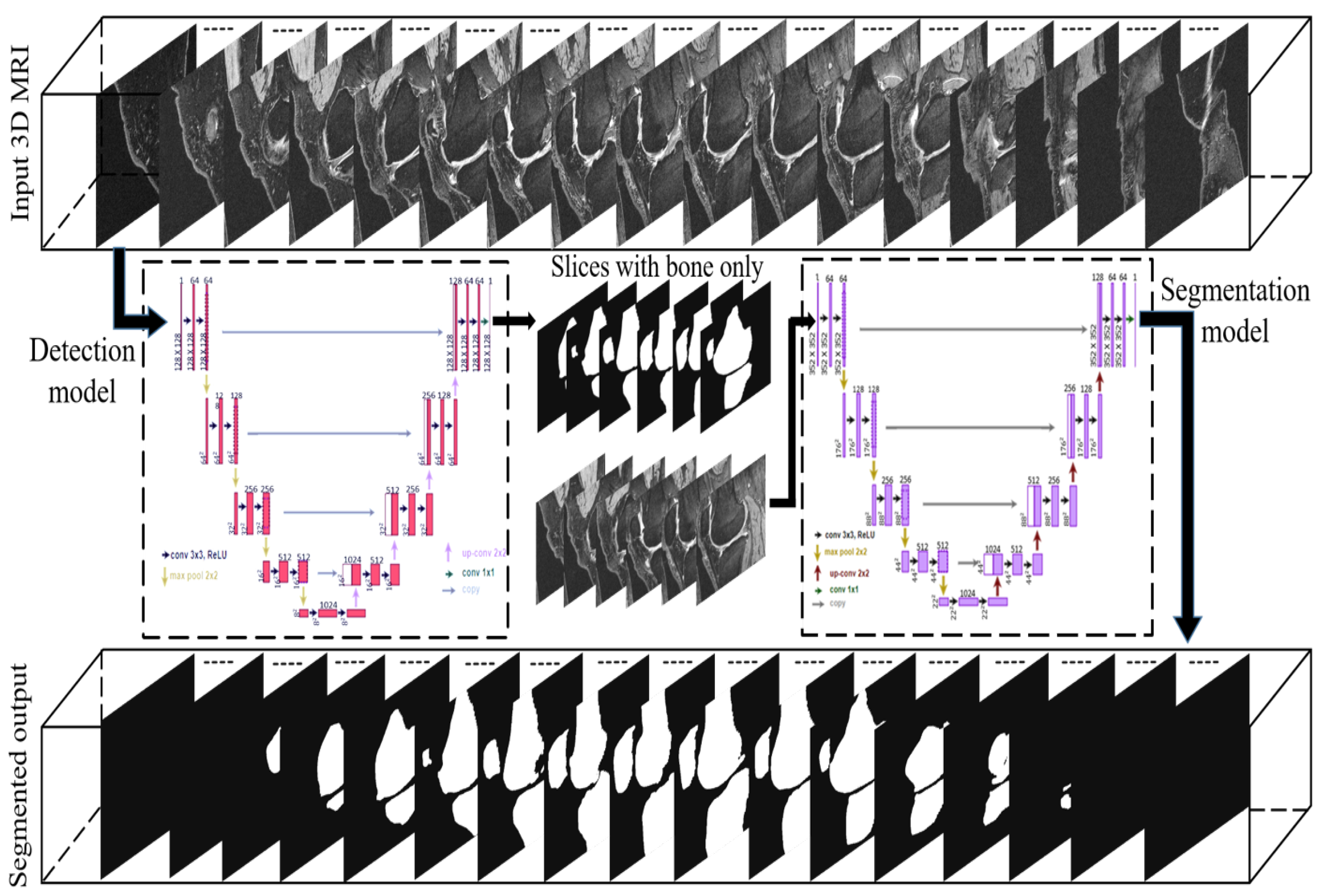
2. Materials and Methods
2.1. Dataset
2.2. Deep Convolutional Networks
2.3. U-Net
2.4. Generation of Training and Testing Sets
2.5. Implementation
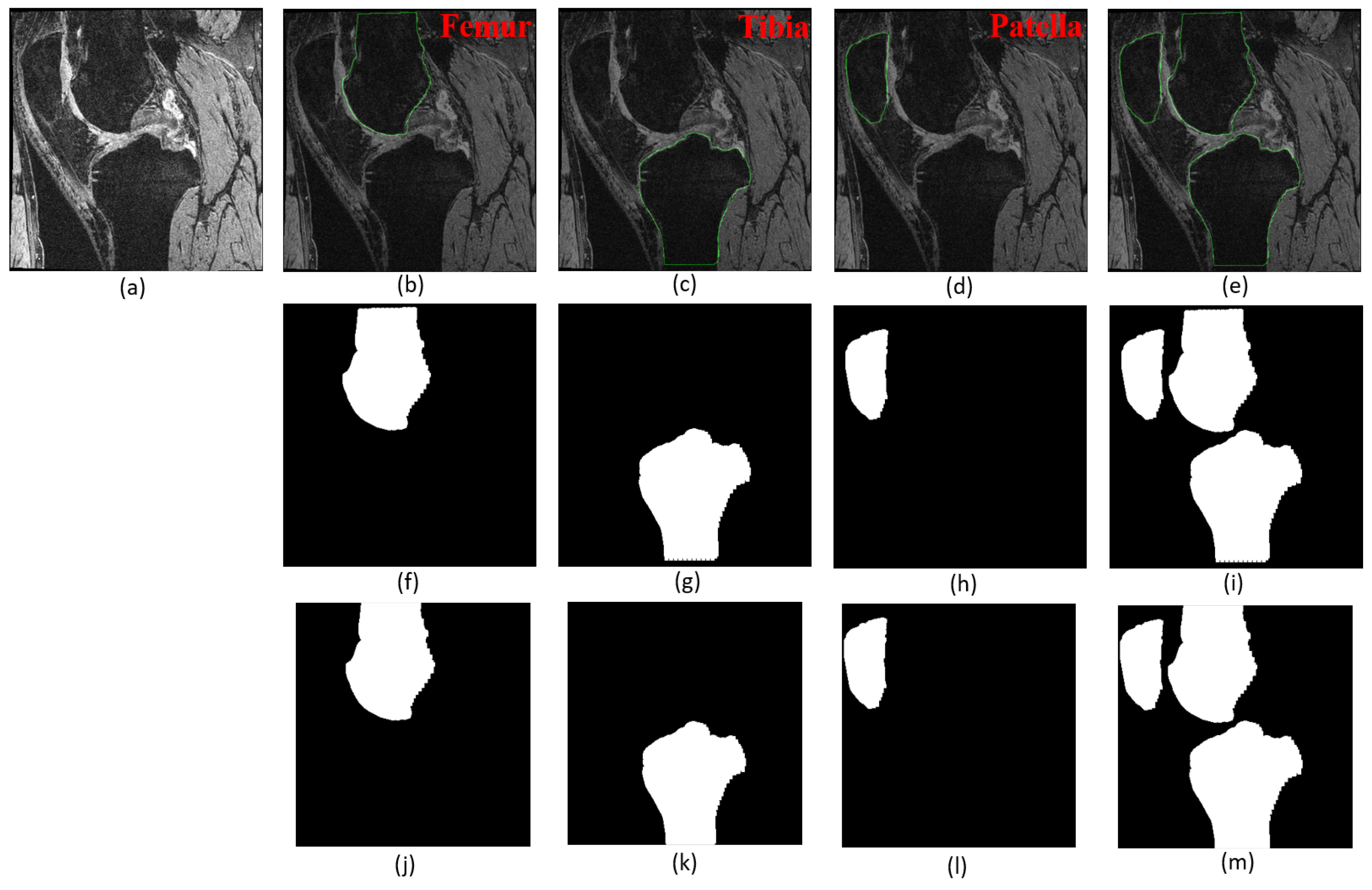
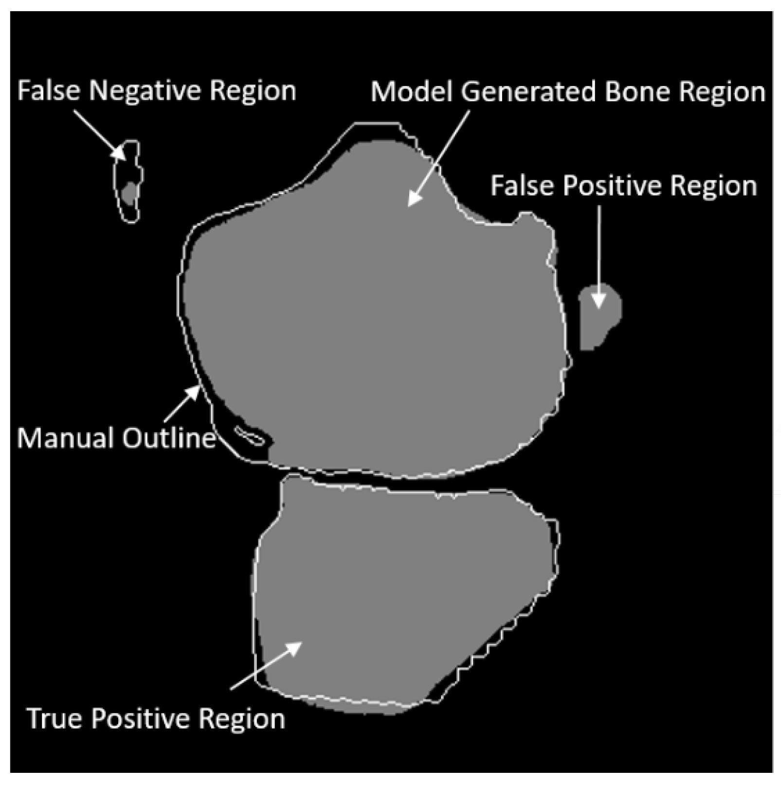
3. Results
3.1. Evaluation Metrics
3.2. Experiments
3.2.1. Bone Slice Detection Performance
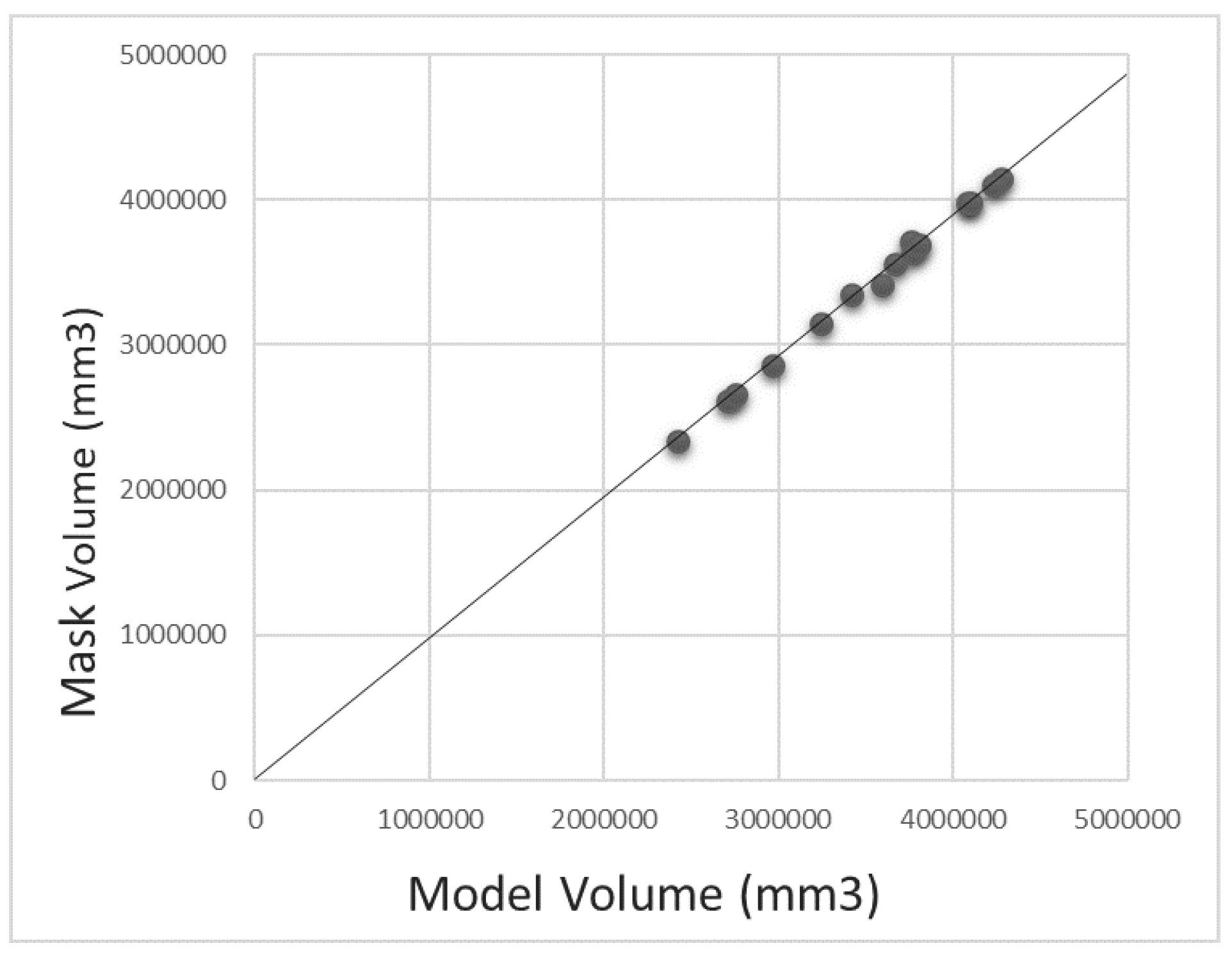
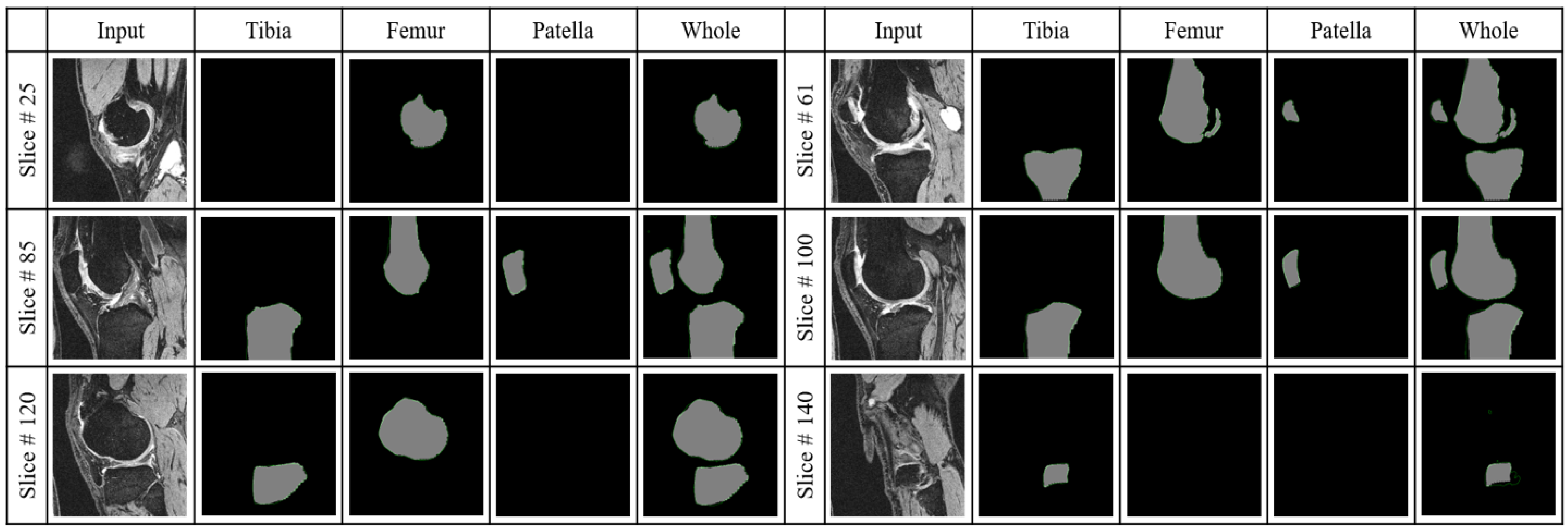
3.2.2. Segmentation Performance
3.2.3. Ablation Study
3.2.4. Whole Knee Model versus Individual Models
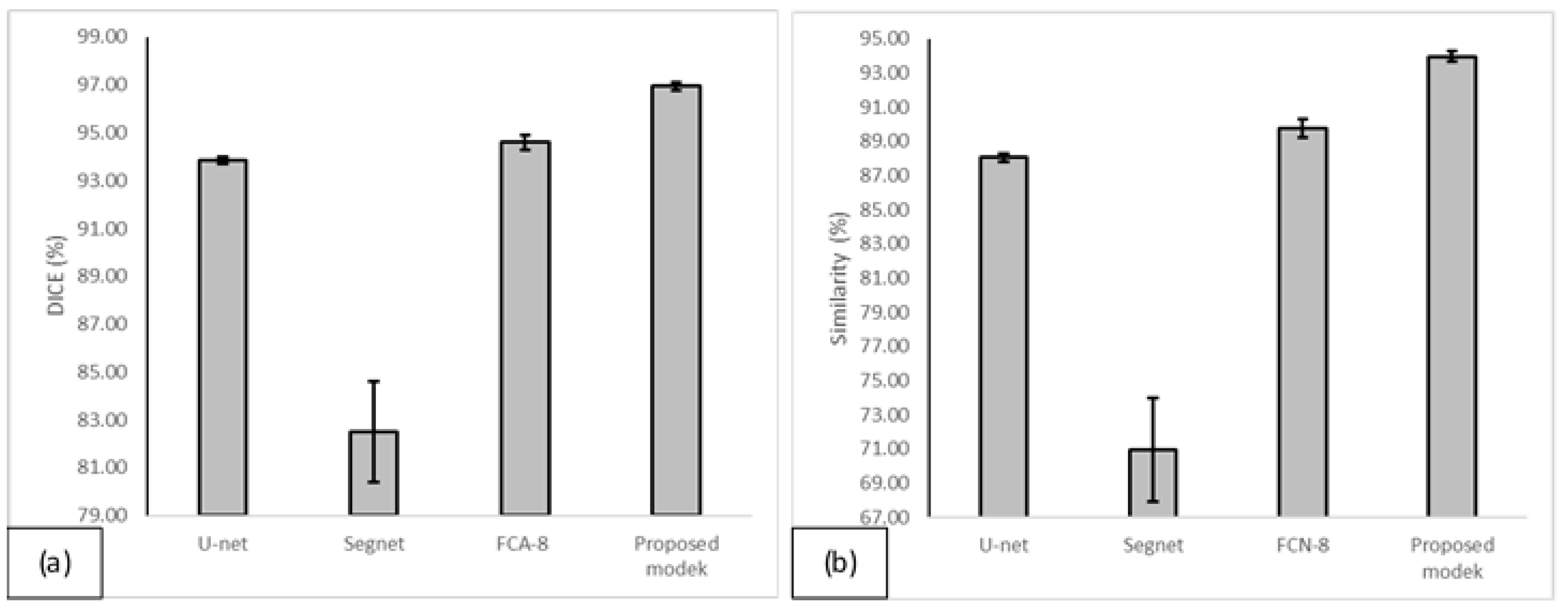
3.2.5. The Proposed Model versus Other State-of-the-Art Models
4. Discussion
5. Conclusions
Author Contributions
Funding
Institutional Review Board Statement
Informed Consent Statement
Data Availability Statement
Conflicts of Interest
References
- Losina, E.; Daigle, M.E.; Suter, L.; Hunter, D.; Solomon, D.; Walensky, R.; Jordan, J.; Burbine, S.A.; Paltiel, A.D.; Katz, J.N. Disease-modifying drugs for knee osteoarthritis: Can they be cost-effective? Osteoarthr. Cartil. 2013, 21, 655–667. [Google Scholar] [CrossRef] [PubMed]
- Felson, D.T. Osteoarthritis as a disease of mechanics. Osteoarthr. Cartil. 2013, 21, 10–15. [Google Scholar] [CrossRef]
- Felson, D.T.; Lawrence, R.C.; Dieppe, P.A.; Hirsch, R.; Helmick, C.G.; Jordan, J.M.; Kington, R.S.; Lane, N.E.; Nevitt, M.C.; Zhang, Y.; et al. Osteoarthritis: New insights. Part 1: The disease and its risk factors. Ann. Intern. Med. 2000, 133, 635–646. [Google Scholar] [CrossRef] [PubMed]
- National Institutes of Health. Osteoarthritis Initiative Releases First Data; News Releases; US Department of Health & Human Services: Bethesda, MD, USA, 2006.
- Yelin, E.; Weinstein, S.; King, T. The Burden of Musculoskeletal Diseases in the United States; Seminars in Arthritis and Rheumatism; Elsevier: Amsterdam, The Netherlands, 2016; Volume 46, pp. 259–260. [Google Scholar]
- Losina, E.; Paltiel, A.D.; Weinstein, A.M.; Yelin, E.; Hunter, D.J.; Chen, S.P.; Klara, K.; Suter, L.G.; Solomon, D.H.; Burbine, S.A.; et al. Lifetime medical costs of knee osteoarthritis management in the United States: Impact of extending indications for total knee arthroplasty. Arthritis Care Res. 2015, 67, 203–215. [Google Scholar] [CrossRef]
- Jevsevar, D.S. Treatment of osteoarthritis of the knee: Evidence-based guideline. JAAOS-J. Am. Acad. Orthop. Surg. 2013, 21, 571–576. [Google Scholar]
- Guccione, A.A.; Felson, D.T.; Anderson, J.J.; Anthony, J.M.; Zhang, Y.; Wilson, P.W.; Kelly-Hayes, M.; Wolf, P.A.; Kreger, B.E.; Kannel, W.B. The effects of specific medical conditions on the functional limitations of elders in the Framingham Study. Am. J. Public Health 1994, 84, 351–358. [Google Scholar] [CrossRef]
- Heidari, B. Knee osteoarthritis prevalence, risk factors, pathogenesis and features: Part I. Casp. J. Intern. Med. 2011, 2, 205. [Google Scholar]
- Bhatia, D.; Bejarano, T.; Novo, M. Current interventions in the management of knee osteoarthritis. J. Pharm. Bioallied Sci. 2013, 5, 30. [Google Scholar] [CrossRef]
- Chan, W.P.; Lang, P.; Stevens, M.P.; Sack, K.; Majumdar, S.; Stoller, D.W.; Basch, C.; Genant, H.K. Osteoarthritis of the knee: Comparison of radiography, CT, and MR imaging to assess extent and severity. AJR. Am. J. Roentgenol. 1991, 157, 799–806. [Google Scholar] [CrossRef]
- Eckstein, F.; Cicuttini, F.; Raynauld, J.P.; Waterton, J.C.; Peterfy, C. Magnetic resonance imaging (MRI) of articular cartilage in knee osteoarthritis (OA): Morphological assessment. Osteoarthr. Cartil. 2006, 14, 46–75. [Google Scholar] [CrossRef]
- Eckstein, F.; Burstein, D.; Link, T.M. Quantitative MRI of cartilage and bone: Degenerative changes in osteoarthritis. NMR Biomed. 2006, 19, 822–854. [Google Scholar] [CrossRef]
- Jaremko, J.; Cheng, R.; Lambert, R.; Habib, A.; Ronsky, J. Reliability of an efficient MRI-based method for estimation of knee cartilage volume using surface registration. Osteoarthr. Cartil. 2006, 14, 914–922. [Google Scholar] [CrossRef]
- Boesen, M.; Ellegaard, K.; Henriksen, M.; Gudbergsen, H.; Hansen, P.; Bliddal, H.; Bartels, E.; Riis, R. Osteoarthritis year in review 2016: Imaging. Osteoarthr. Cartil. 2017, 25, 216–226. [Google Scholar] [CrossRef]
- Yin, Y.; Zhang, X.; Williams, R.; Wu, X.; Anderson, D.D.; Sonka, M. LOGISMOS—Layered optimal graph image segmentation of multiple objects and surfaces: Cartilage segmentation in the knee joint. IEEE Trans. Med. Imaging 2010, 29, 2023–2037. [Google Scholar] [CrossRef]
- Fripp, J.; Crozier, S.; Warfield, S.K.; Ourselin, S. Automatic segmentation and quantitative analysis of the articular cartilages from magnetic resonance images of the knee. IEEE Trans. Med. Imaging 2009, 29, 55–64. [Google Scholar] [CrossRef] [PubMed]
- Eckstein, F.; Wirth, W. Quantitative cartilage imaging in knee osteoarthritis. Arthritis 2011, 2011, 475684. [Google Scholar] [CrossRef] [PubMed]
- Tameem, H.Z.; Sinha, U.S. Automated image processing and analysis of cartilage MRI: Enabling technology for data mining applied to osteoarthritis. In Proceedings of the AIP Conference Proceedings, Gainesville, FL, USA, 28–30 March 2007; American Institute of Physics Inc.: Woodbury, NY, USA, 2007; Volume 953, pp. 262–276. [Google Scholar]
- Cashman, P.M.; Kitney, R.I.; Gariba, M.A.; Carter, M.E. Automated techniques for visualization and mapping of articular cartilage in MR images of the osteoarthritic knee: A base technique for the assessment of microdamage and submicro damage. IEEE Trans. Nanobioscience 2002, 99, 42–51. [Google Scholar] [CrossRef] [PubMed]
- Vincent, G.; Wolstenholme, C.; Scott, I.; Bowes, M. Fully automatic segmentation of the knee joint using active appearance models. Med. Image Anal. Clin. Grand Chall. 2010, 1, 224. [Google Scholar]
- Lee, H.; Pham, P.; Largman, Y.; Ng, A. Unsupervised feature learning for audio classification using convolutional deep belief networks. Adv. Neural Inf. Process. Syst. 2009, 22, 1096–1104. [Google Scholar]
- Lee, H.; Grosse, R.; Ranganath, R.; Ng, A.Y. Convolutional deep belief networks for scalable unsupervised learning of hierarchical representations. In Proceedings of the 26th Annual International Conference on Machine Learning, Montreal, QC, Canada, 14–18 June 2009; pp. 609–616. [Google Scholar]
- Le, Q.V.; Zou, W.Y.; Yeung, S.Y.; Ng, A.Y. Learning hierarchical invariant spatio-temporal features for action recognition with independent subspace analysis. In Proceedings of the IEEE Computer Vision and Pattern Recognition (CVPR), Colorado Springs, CO, USA, 20–25 June 2011; pp. 3361–3368. [Google Scholar]
- Cruz-Roa, A.A.; Ovalle, J.E.A.; Madabhushi, A.; Osorio, F.A.G. A deep learning architecture for image representation, visual interpretability and automated basal-cell carcinoma cancer detection. In Proceedings of the International Conference on Medical Image Computing and Computer-Assisted Intervention, Nagoya, Japan, 22–26 September 2013; Springer: Berlin/Heidelberg, Germany, 2013; pp. 403–410. [Google Scholar]
- Lo Giudice, A.; Ronsivalle, V.; Spampinato, C.; Leonardi, R. Fully automatic segmentation of the mandible based on convolutional neural networks (CNNs). Orthod. Craniofacial Res. 2021, 24, 100–107. [Google Scholar] [CrossRef] [PubMed]
- Leonardi, R.; Giudice, A.L.; Farronato, M.; Ronsivalle, V.; Allegrini, S.; Musumeci, G.; Spampinato, C. Fully automatic segmentation of sinonasal cavity and pharyngeal airway based on convolutional neural networks. Am. J. Orthod. Dentofac. Orthop. 2021, 159, 824–835. [Google Scholar] [CrossRef]
- Cherukuri, V.; Ssenyonga, P.; Warf, B.C.; Kulkarni, A.V.; Monga, V.; Schiff, S.J. Learning based segmentation of CT brain images: Application to postoperative hydrocephalic scans. IEEE Trans. Biomed. Eng. 2017, 65, 1871–1884. [Google Scholar]
- Veena, H.; Muruganandham, A.; Kumaran, T.S. A novel optic disc and optic cup segmentation technique to diagnose glaucoma using deep learning convolutional neural network over retinal fundus images. J. King Saud-Univ.-Comput. Inf. Sci. 2021. [Google Scholar] [CrossRef]
- Li, W. Automatic segmentation of liver tumor in CT images with deep convolutional neural networks. J. Comput. Commun. 2015, 3, 146. [Google Scholar] [CrossRef]
- Wang, S.; Zhou, M.; Liu, Z.; Liu, Z.; Gu, D.; Zang, Y.; Dong, D.; Gevaert, O.; Tian, J. Central focused convolutional neural networks: Developing a data-driven model for lung nodule segmentation. Med. Image Anal. 2017, 40, 172–183. [Google Scholar] [CrossRef] [PubMed]
- Ronneberger, O.; Fischer, P.; Brox, T. U-net: Convolutional networks for biomedical image segmentation. In Proceedings of the International Conference on Medical Image Computing and Computer-Assisted Intervention (MICCAI), Munich, Germany, 5–9 October 2015; Springer: Cham, Switzerland, 2015; pp. 234–241. [Google Scholar]
- Gougoutas, A.J.; Wheaton, A.J.; Borthakur, A.; Shapiro, E.M.; Kneeland, J.B.; Udupa, J.K.; Reddy, R. Cartilage volume quantification via Live Wire segmentation1. Acad. Radiol. 2004, 11, 1389–1395. [Google Scholar] [CrossRef]
- Caselles, V.; Kimmel, R.; Sapiro, G. Geodesic active contours. Int. J. Comput. Vis. 1997, 22, 61–79. [Google Scholar] [CrossRef]
- Kass, M.; Witkin, A.; Terzopoulos, D. Snakes: Active contour models. Int. J. Comput. Vis. 1988, 1, 321–331. [Google Scholar] [CrossRef]
- Solloway, S.; Hutchinson, C.E.; Waterton, J.C.; Taylor, C.J. The use of active shape models for making thickness measurements of articular cartilage from MR images. Magn. Reson. Med. 1997, 37, 943–952. [Google Scholar] [CrossRef]
- Duryea, J.; Neumann, G.; Brem, M.; Koh, W.; Noorbakhsh, F.; Jackson, R.; Yu, J.; Eaton, C.; Lang, P. Novel fast semi-automated software to segment cartilage for knee MR acquisitions. Osteoarthr. Cartil. 2007, 15, 487–492. [Google Scholar] [CrossRef][Green Version]
- Adams, R.; Bischof, L. Seeded region growing. IEEE Trans. Pattern Anal. Mach. Intell. 1994, 16, 641–647. [Google Scholar] [CrossRef]
- Dodin, P.; Pelletier, J.P.; Martel-Pelletier, J.; Abram, F. Automatic human knee cartilage segmentation from 3 to D magnetic resonance images. IEEE Trans. Biomed. Eng. 2010, 57, 2699–2711. [Google Scholar] [CrossRef] [PubMed]
- Dodin, P.; Martel-Pelletier, J.; Pelletier, J.P.; Abram, F. A fully automated human knee 3D MRI bone segmentation using the ray casting technique. Med. Biol. Eng. Comput. 2011, 49, 1413–1424. [Google Scholar] [CrossRef] [PubMed]
- Eckstein, F.; Gavazzeni, A.; Sittek, H.; Haubner, M.; Lösch, A.; Milz, S.; Englmeier, K.H.; Schulte, E.; Putz, R.; Reiser, M. Determination of knee joint cartilage thickness using three-dimensional magnetic resonance chondro-crassometry (3D MR-CCM). Magn. Reson. Med. 1996, 36, 256–265. [Google Scholar] [CrossRef] [PubMed]
- Grau, V.; Mewes, A.; Alcaniz, M.; Kikinis, R.; Warfield, S.K. Improved watershed transform for medical image segmentation using prior information. IEEE Trans. Med. Imaging 2004, 23, 447–458. [Google Scholar] [CrossRef]
- Ambellan, F.; Tack, A.; Ehlke, M.; Zachow, S. Automated segmentation of knee bone and cartilage combining statistical shape knowledge and convolutional neural networks: Data from the Osteoarthritis Initiative. Med. Image Anal. 2019, 52, 109–118. [Google Scholar] [CrossRef] [PubMed]
- Almajalid, R.; Shan, J.; Zhang, M.; Stonis, G.; Zhang, M. Knee bone segmentation on three-dimensional MRI. In Proceedings of the 2019 18th IEEE International Conference On Machine Learning and Applications (ICMLA), Boca Raton, FL, USA, 16–19 December 2019; pp. 1725–1730. [Google Scholar]
- Liu, F.; Zhou, Z.; Jang, H.; Samsonov, A.; Zhao, G.; Kijowski, R. Deep convolutional neural network and 3D deformable approach for tissue segmentation in musculoskeletal magnetic resonance imaging. Magn. Reson. Med. 2018, 79, 2379–2391. [Google Scholar] [CrossRef] [PubMed]
- Liu, F. SUSAN: Segment unannotated image structure using adversarial network. Magn. Reson. Med. 2019, 81, 3330–3345. [Google Scholar] [CrossRef] [PubMed]
- Wu, D.; Sofka, M.; Birkbeck, N.; Zhou, S.K. Segmentation of multiple knee bones from CT for orthopedic knee surgery planning. In Proceedings of the International Conference on Medical Image Computing and Computer-Assisted Intervention (MICCAI), Boston, MA, USA, 14–18 September 2014; Springer International Publishing: Cham, Switzerland, 2014; pp. 372–380. [Google Scholar]
- Balsiger, F.; Ronchetti, T.; Pletscher, M. Distal Femur Segmentation on MR Images Using Random Forests; Medical Image Analysis Laboratory: Burnaby, BC, Canada, 2015. [Google Scholar]
- Imorphics. Available online: http://imorphics.com/ (accessed on 30 July 2021).
- LeCun, Y.; Bottou, L.; Bengio, Y.; Haffner, P. Gradient-based learning applied to document recognition. Proc. IEEE 1998, 86, 2278–2324. [Google Scholar] [CrossRef]
- Girshick, R.; Donahue, J.; Darrell, T.; Malik, J. Rich feature hierarchies for accurate object detection and semantic segmentation. In Proceedings of the IEEE Conference on Computer Vision and Pattern Recognition (CVPR), Columbus, OH, USA, 24–27 June 2014; pp. 580–587. [Google Scholar]
- Krizhevsky, A.; Sutskever, I.; Hinton, G.E. Imagenet classification with deep convolutional neural networks. Adv. Neural Inf. Process. Syst. 2012, 25, 1097–1105. [Google Scholar] [CrossRef]
- Kingma, D.P.; Ba, J. Adam: A method for stochastic optimization. arXiv 2014, arXiv:1412.6980. [Google Scholar]
- Chollet, F. Keras. Available online: https://github.com/fchollet/keras (accessed on 30 July 2021).
- Abadi, M.; Agarwal, A.; Barham, P.; Brevdo, E.; Chen, Z.; Citro, C.; Corrado, G.S.; Davis, A.; Dean, J.; Devin, M.; et al. Tensorflow: Large-scale machine learning on heterogeneous distributed systems. arXiv 2016, arXiv:1603.04467. [Google Scholar]
- Dice, L.R. Measures of the amount of ecologic association between species. Ecology 1945, 26, 297–302. [Google Scholar] [CrossRef]
- Badrinarayanan, V.; Kendall, A.; Cipolla, R. SegNet: A deep convolutional encoder-decoder architecture for image segmentation. IEEE Trans. Pattern Anal. Mach. Intell. 2017, 39, 2481–2495. [Google Scholar] [CrossRef] [PubMed]
- Long, J.; Shelhamer, E.; Darrell, T. Fully convolutional networks for semantic segmentation. In Proceedings of the IEEE Conference on Computer Vision and Pattern Recognition (CVPR), Boston, MA, USA, 7–12 June 2015; pp. 3431–3440. [Google Scholar]


| Paper | Year | Approach | Dataset | Region of Interest | Performance | Advantages | Drawbacks |
|---|---|---|---|---|---|---|---|
| Wu, et al. [47] | 2014 | MSL, SSM, Graph cut | 465 CT scans | FB, TB, PB, FiB | AvgD: FB-0.82 mm, TB-0.96 mm, PB-0.68 mm, FiB-0.96 mm | High accuracy of overlap removal for bones | Boundary leakage |
| Fabian et al. [48] | 2015 | Random forest classifier | 20 MRI | FB | DICE: 92.37% Sens: 91.75% Spec: 99.29% | Short training time | Smaller dataset used, classification accuracy relied heavily on the quality of labeled data |
| Liu et al. [45] | 2018 | SegNet, 3D deformable model | 100 MRI (SKI10) | FB, FC, TB, TC | AvgD: FB-0.56 mm, TB-0.50 mm, VOE: FC-28.4%, TC-33.1% | Low computation cost, short training time | Compared SegNet with only U-Net |
| Liu [46] | 2018 | R-Net | 60 MRI (SKI10), 2 clinical MRI datasets | FB, FC, TB, TC | DICE: FB-97.0%, TB-95.0%, FC-81.0%, TC-75.0% | The first study to translate one MRI sequence to another | No comparison with other techniques |
| Ambellan et al. [44] | 2019 | U-net, SSM | 100 MRI (SKI10), 88 (OAI Imorphics), 507 (OAI-ZIB) | FB, FC, TB, TC | DICE: FB-98.6%, TB-98.5%, FC-89.9%, TC-85.6% | Achieved good segmentation accuracy, time-efficient | Compromise between memory and size for choosing subvolume to train 3D CNN |
| FP | FN | TP | TN | Recall | Precision | Accuracy (%) | |
|---|---|---|---|---|---|---|---|
| Tibia | 20 | 9 | 1679 | 692 | 0.995 | 0.988 | 98.79 |
| Femur | 20 | 8 | 1786 | 586 | 0.996 | 0.988 | 98.83 |
| Patella | 9 | 28 | 950 | 1413 | 0.971 | 0.992 | 98.46 |
| Whole Knee | 20 | 9 | 1831 | 540 | 0.995 | 0.989 | 98.79 |
| TPR (%) | FPR (%) | FNR (%) | SI (%) | DICE (%) | |
|---|---|---|---|---|---|
| Tibia | 96.93 | 3.27 | 3.07 | 93.87 | 96.83 |
| Femur | 98.26 | 2.46 | 1.74 | 95.91 | 97.92 |
| Patella | 96.45 | 11.50 | 3.55 | 86.61 | 92.83 |
| Whole Knee | 98.51 | 4.83 | 1.49 | 93.98 | 96.94 |
| TPR (%) | FPR (%) | FNR (%) | SI (%) | DICE (%) | |
|---|---|---|---|---|---|
| Tibia | 97.78 | 3.99 | 2.23 | 94.03 | 96.96 |
| Femur | 97.69 | 2.09 | 2.31 | 95.25 | 98.06 |
| Patella | 95.37 | 6.36 | 4.63 | 89.71 | 94.52 |
| Whole Knee | 98.60 | 4.74 | 1.40 | 94.14 | 97.02 |
| With Manual Detection | With Automatic Detection | p-Value | p-Value | |||
|---|---|---|---|---|---|---|
| SI (%) | DICE (%) | SI (%) | DICE (%) | (DICE) | (SI) | |
| Tibia | 94.03 | 96.96 | 93.87 | 96.83 | 0.400 | 0.729 |
| Femur | 95.25 | 98.06 | 95.91 | 97.92 | 0.399 | 0.330 |
| Patella | 89.71 | 94.52 | 86.61 | 92.83 | 0.304 | 0.239 |
| Whole Knee | 94.14 | 97.02 | 93.98 | 96.94 | 0.489 | 0.499 |
| TPR (%) | FPR (%) | FNR (%) | SI (%) | DICE (%) | |
|---|---|---|---|---|---|
| Whole knee model | 98.60 | 4.74 | 1.40 | 94.14 | 97.02 |
| Combination of three models | 97.66 | 03.29 | 02.34 | 94.55 | 97.20 |
| TPR (%) | FPR (%) | FNR (%) | SI (%) | DICE (%) | |
|---|---|---|---|---|---|
| U-net | 99.67 | 14.08 | 0.33 | 87.38 | 93.26 |
| SegNet | 83.17 | 20.16 | 16.83 | 70.96 | 82.49 |
| FCN-8 | 92.66 | 3.20 | 7.34 | 89.77 | 94.60 |
| Proposed Method | 98.51 | 4.83 | 1.49 | 93.98 | 96.94 |
| Proposed Method | FCN-8 | p-Value | p-Value | ||
|---|---|---|---|---|---|
| SI (%) | DICE (%) | SI (%) | DICE (%) | (DICE) | (SI) |
| 93.98 | 96.94 | 89.77 | 94.60 | 0.0000077 | 0.0000069 |
Publisher’s Note: MDPI stays neutral with regard to jurisdictional claims in published maps and institutional affiliations. |
© 2022 by the authors. Licensee MDPI, Basel, Switzerland. This article is an open access article distributed under the terms and conditions of the Creative Commons Attribution (CC BY) license (https://creativecommons.org/licenses/by/4.0/).
Share and Cite
Almajalid, R.; Zhang, M.; Shan, J. Fully Automatic Knee Bone Detection and Segmentation on Three-Dimensional MRI. Diagnostics 2022, 12, 123. https://doi.org/10.3390/diagnostics12010123
Almajalid R, Zhang M, Shan J. Fully Automatic Knee Bone Detection and Segmentation on Three-Dimensional MRI. Diagnostics. 2022; 12(1):123. https://doi.org/10.3390/diagnostics12010123
Chicago/Turabian StyleAlmajalid, Rania, Ming Zhang, and Juan Shan. 2022. "Fully Automatic Knee Bone Detection and Segmentation on Three-Dimensional MRI" Diagnostics 12, no. 1: 123. https://doi.org/10.3390/diagnostics12010123
APA StyleAlmajalid, R., Zhang, M., & Shan, J. (2022). Fully Automatic Knee Bone Detection and Segmentation on Three-Dimensional MRI. Diagnostics, 12(1), 123. https://doi.org/10.3390/diagnostics12010123