
Inter-Variability Study of COVLIAS 1.0: Hybrid Deep Learning Models for COVID-19 Lung Segmentation in Computed Tomography


 ,
, 
 , ,
, ,  ,
,  ,
,  ,
,  , , , ,
  and
and
Abstract
:1. Introduction
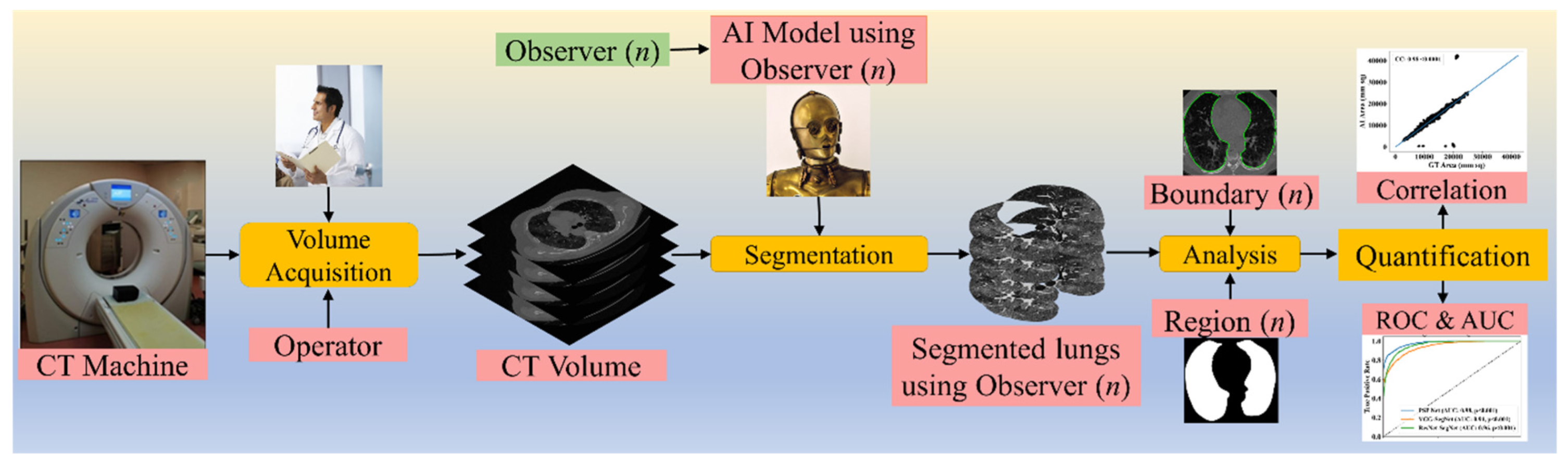
2. Methodology
2.1. Patient Demographics, Image Acquisition, and Data Preparation
2.1.1. Demographics
2.1.2. Image Acquisition
2.1.3. Data Preparation
2.2. Architecture
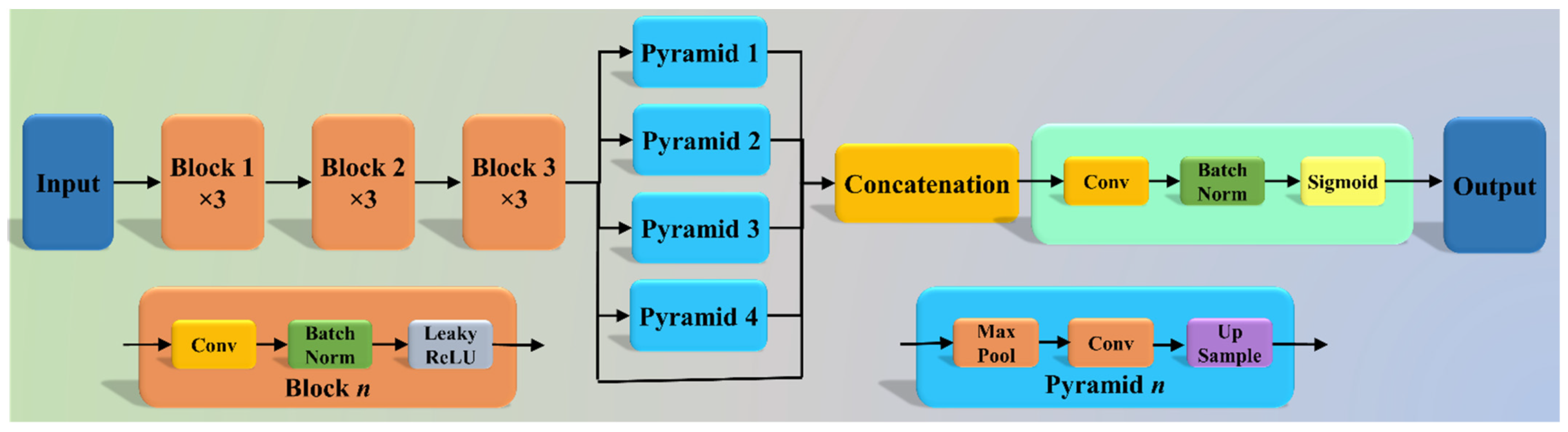
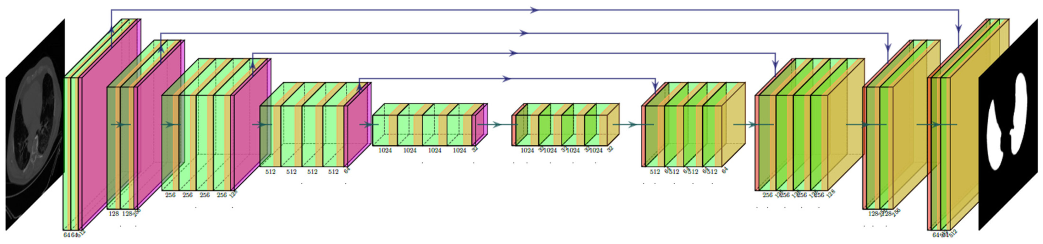
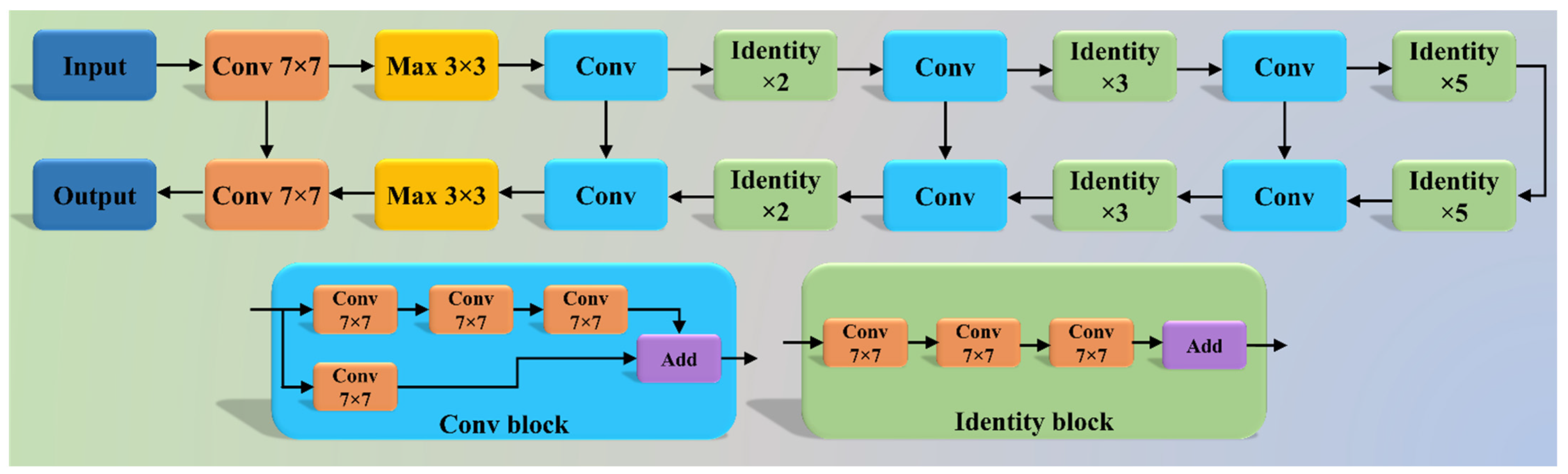
2.2.1. Three AI Models: PSP Net, VGG-SegNet, and ResNet-SegNet
2.2.2. Loss Functions for AI Models
3. Experimental Protocol
3.1. Accuracy Estimation of AI Models Using Cross-Validation
3.2. Lung Quantification
3.3. AI Model Accuracy Computation
4. Results and Performance Evaluation
4.1. Results
4.2. Performance Evaluation
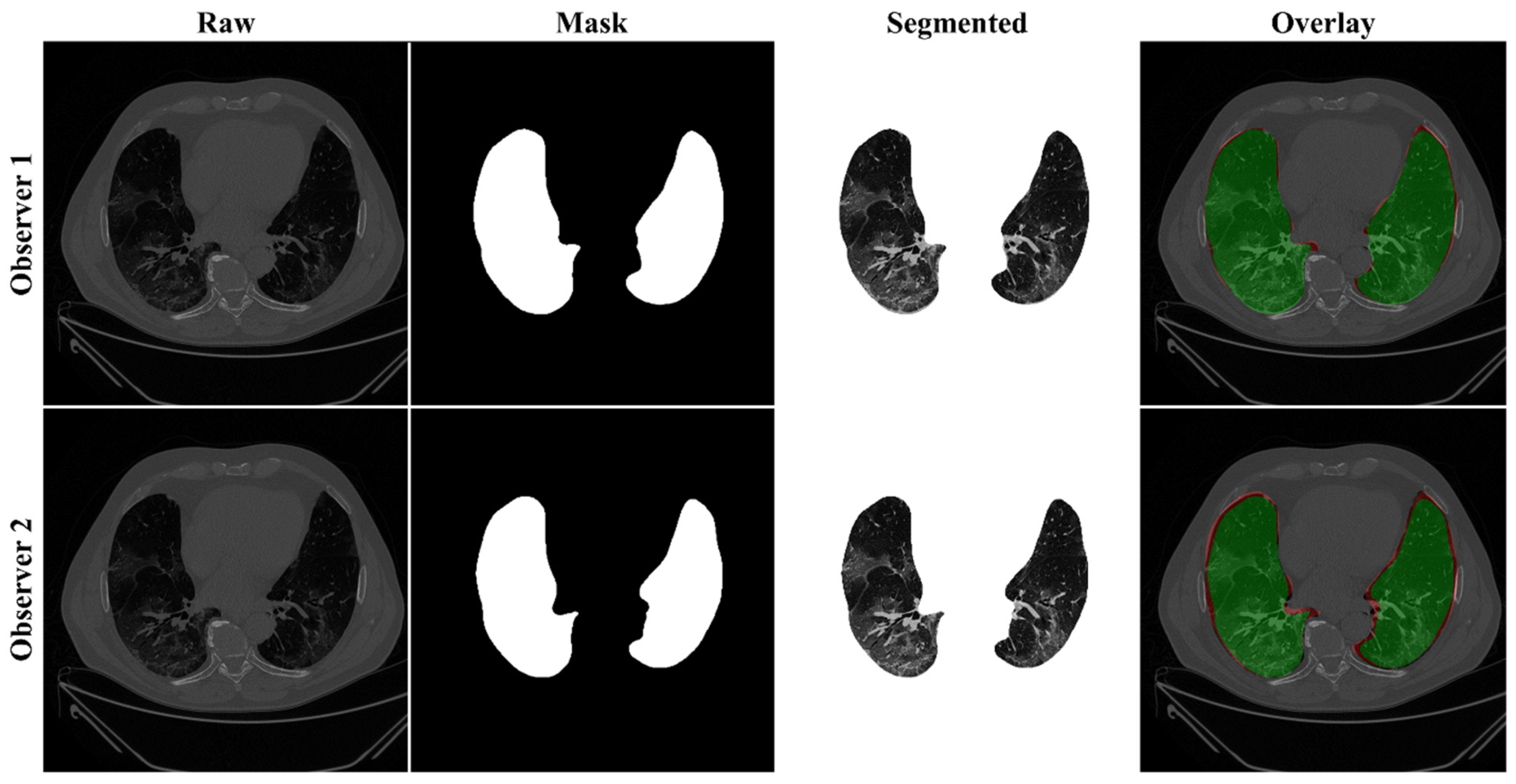
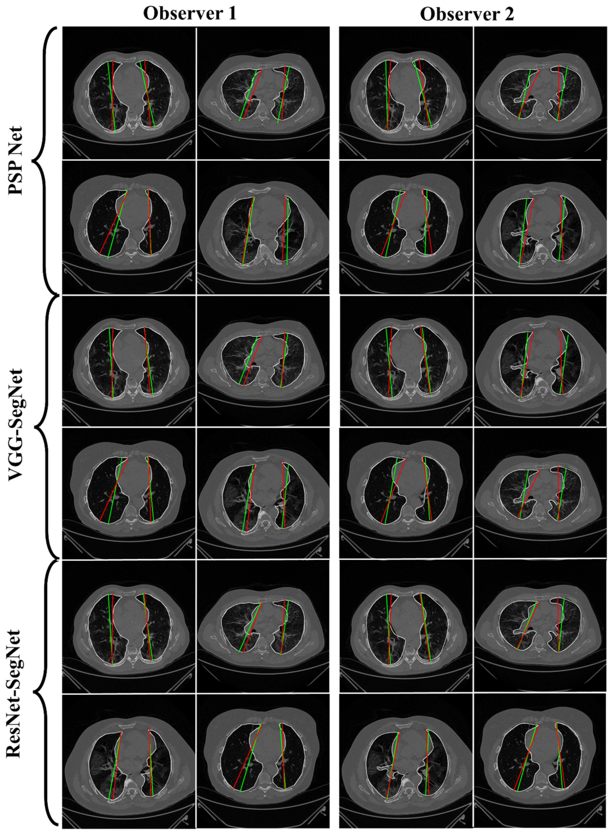
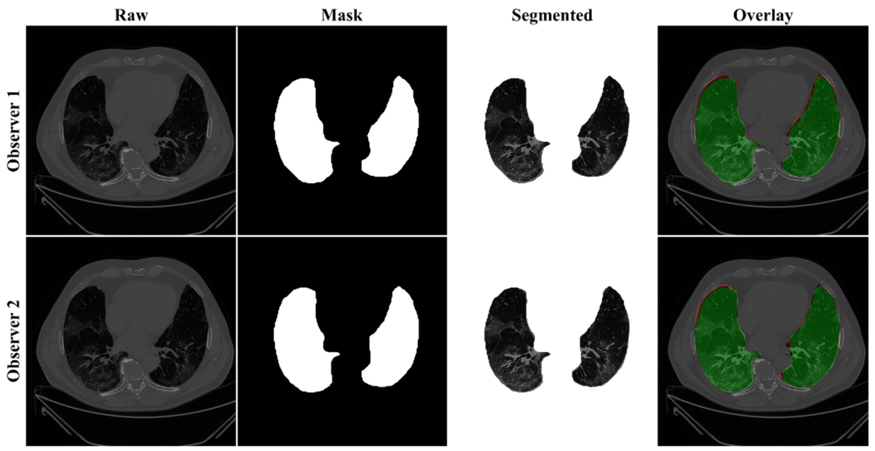
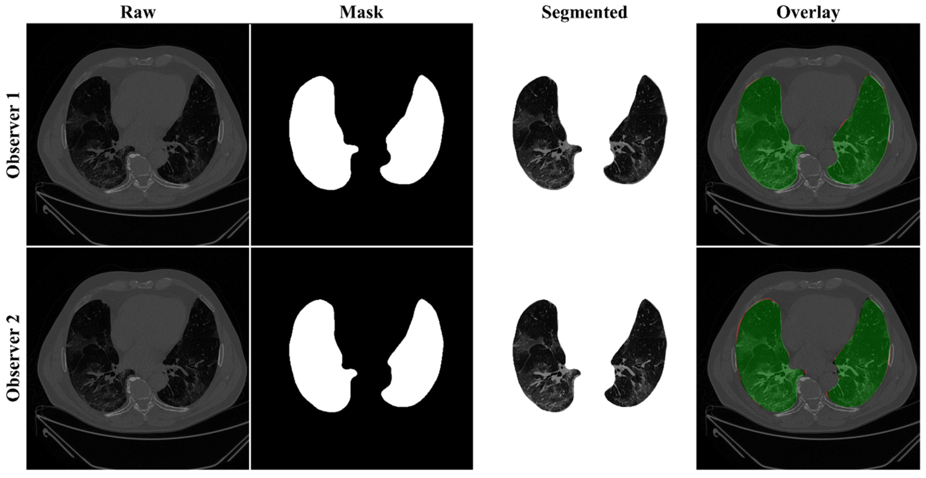
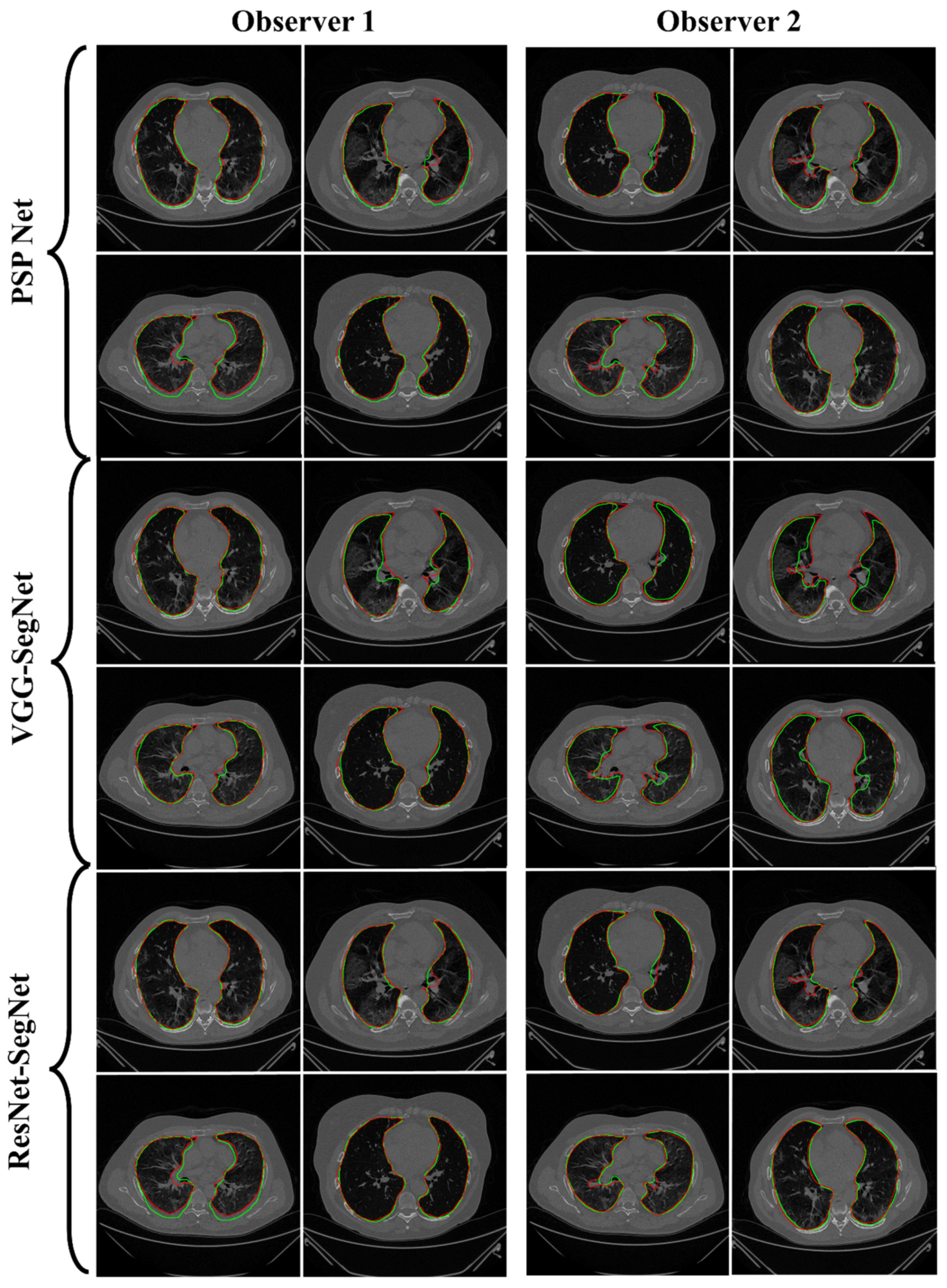
4.2.1. Lung Boundary and Long Axis Visualization
4.2.2. Performance Metrics for the Lung Area Error
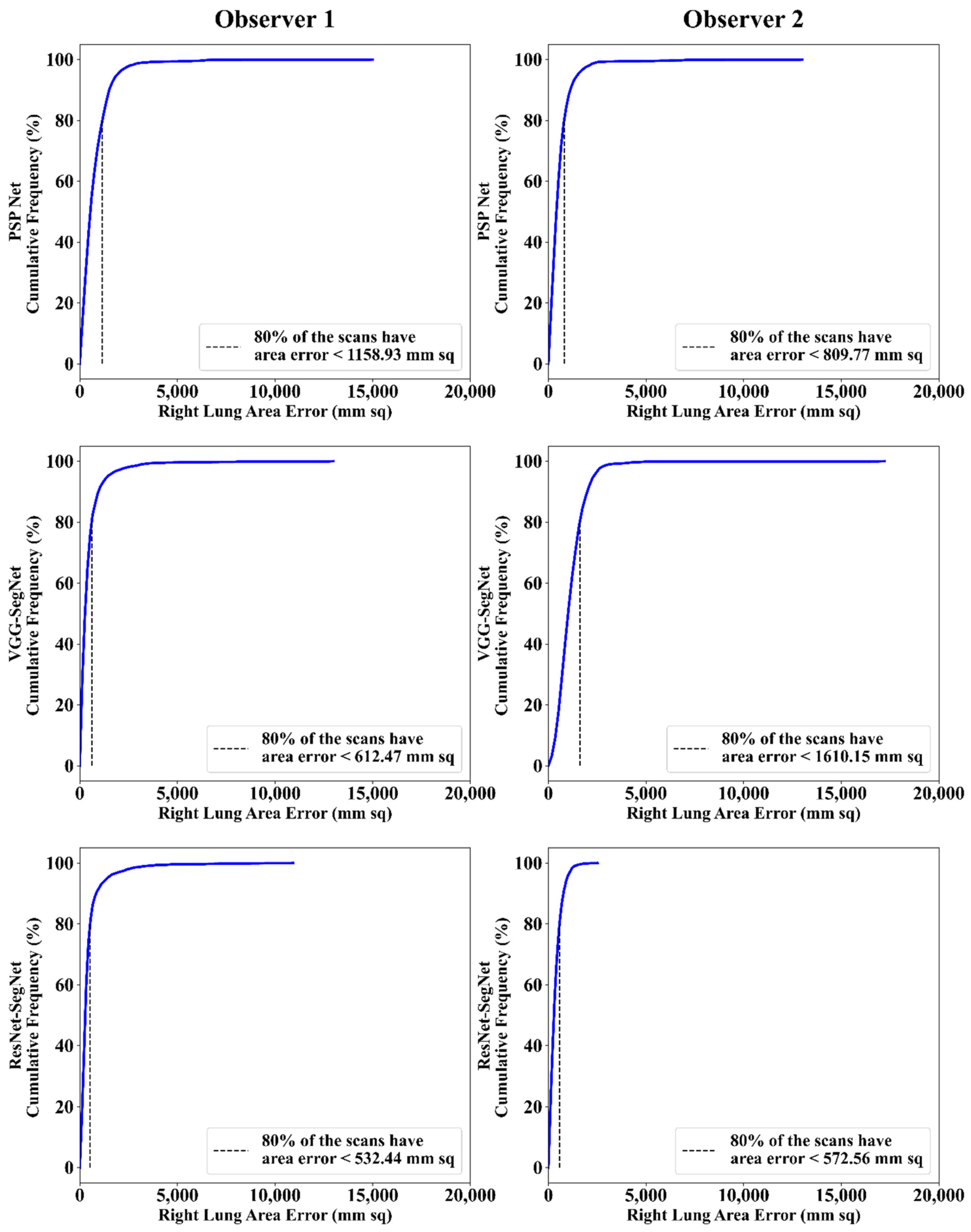
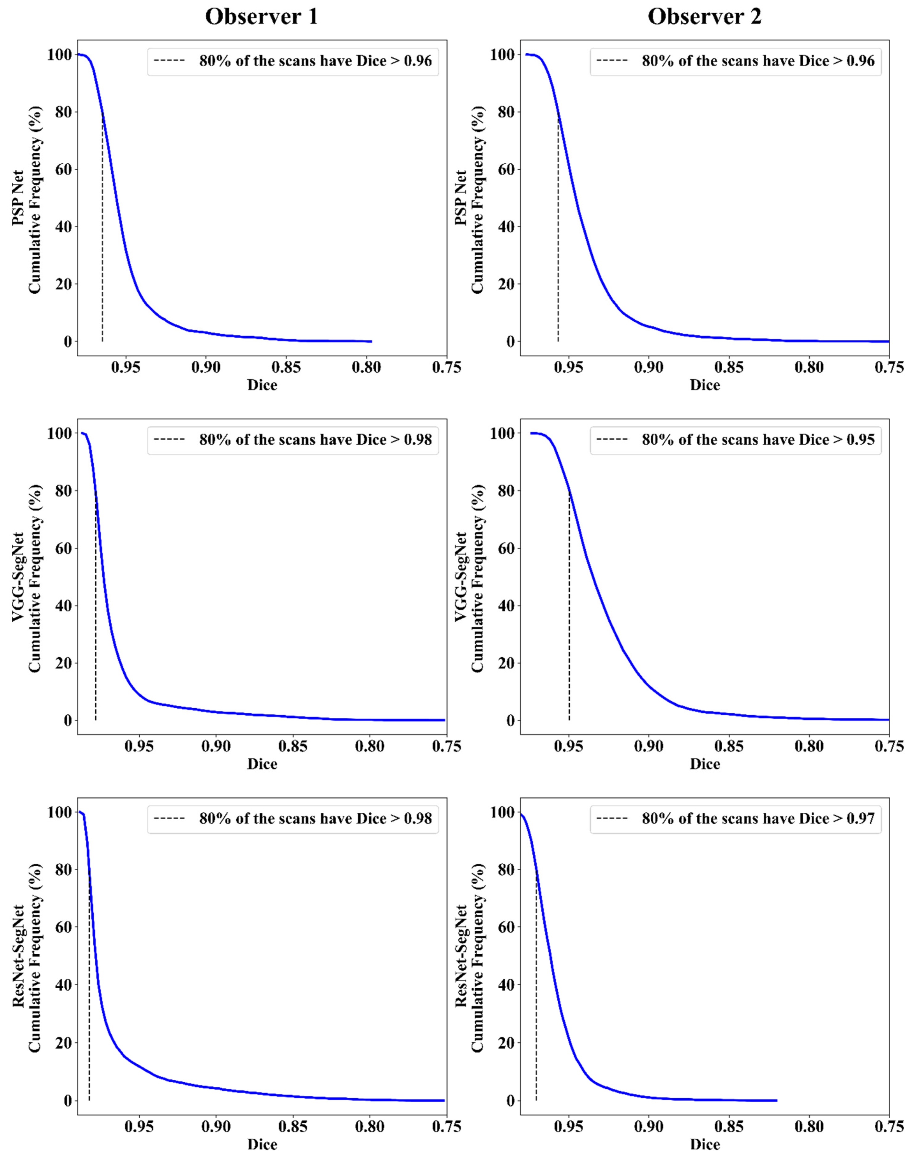
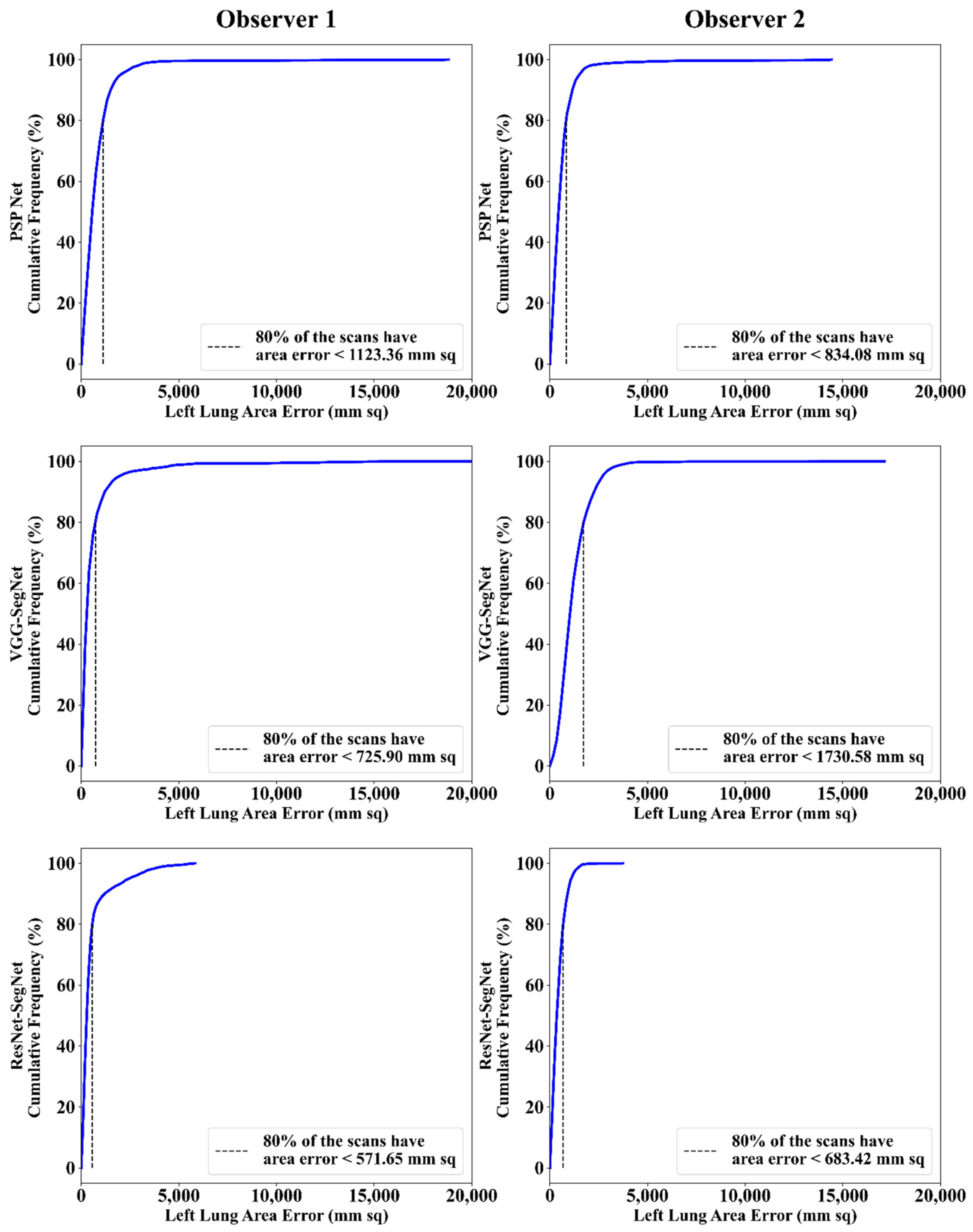
Cumulative Frequency Plot for Lung Area Error
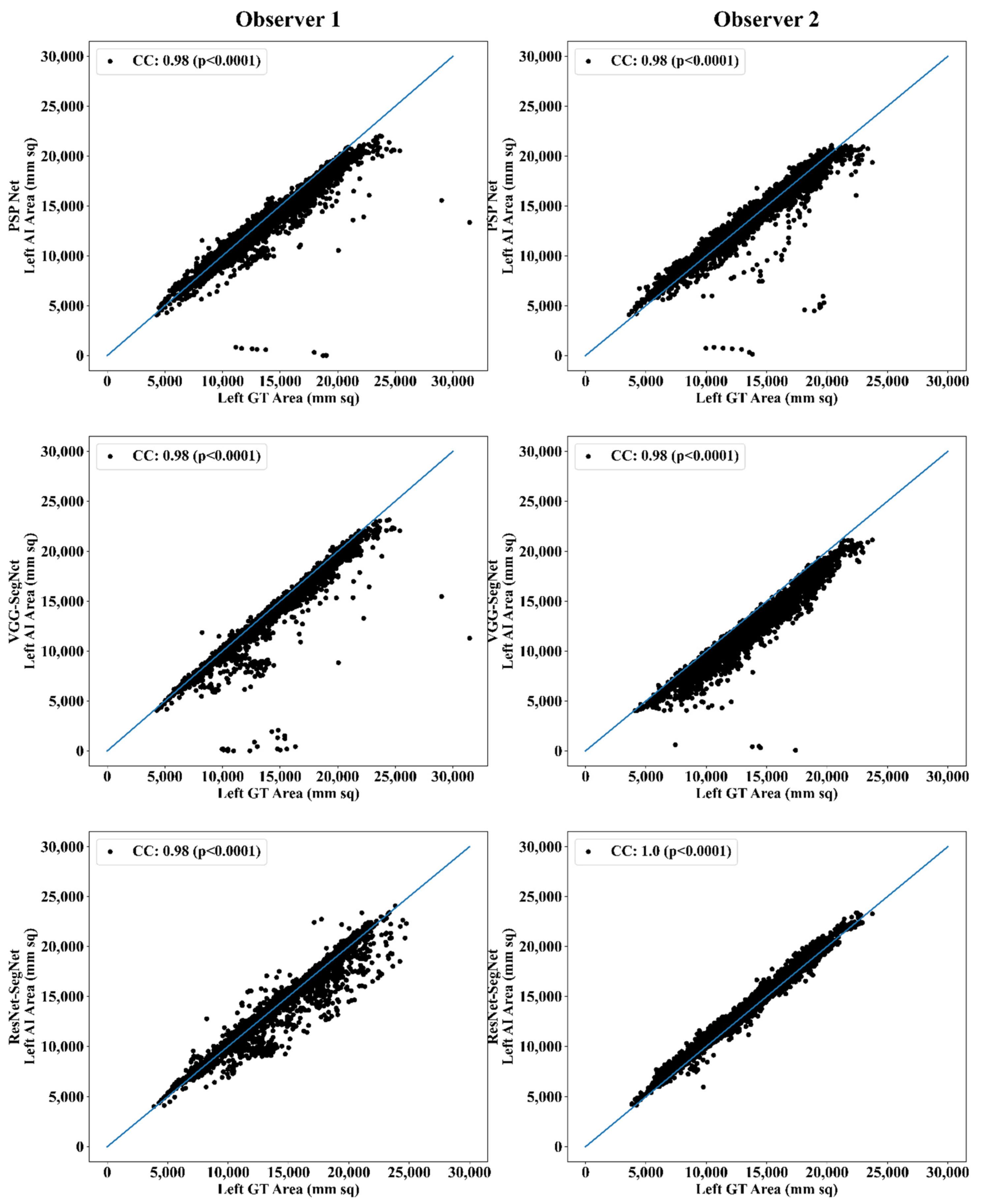
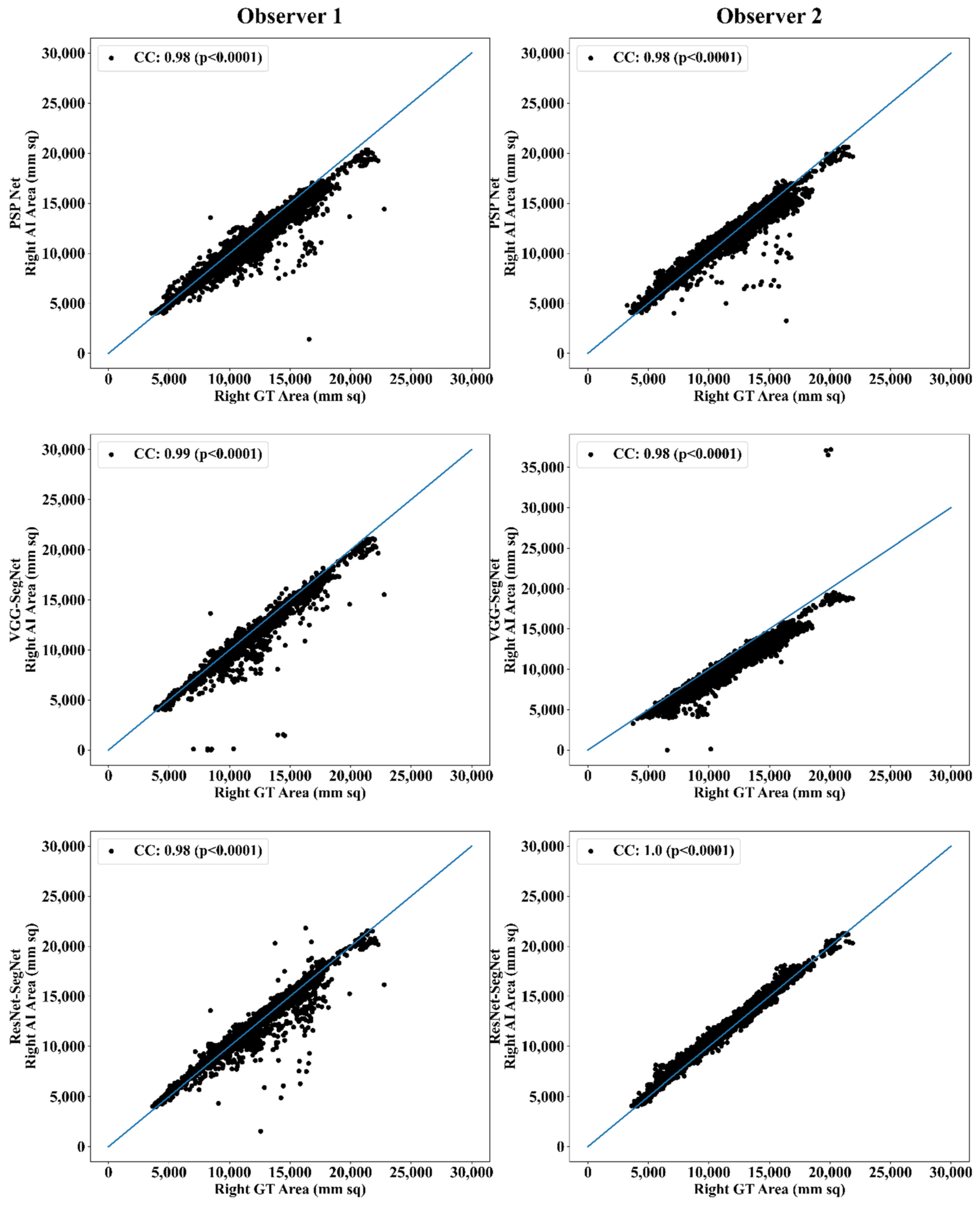
Correlation Plot for Lung Area Error
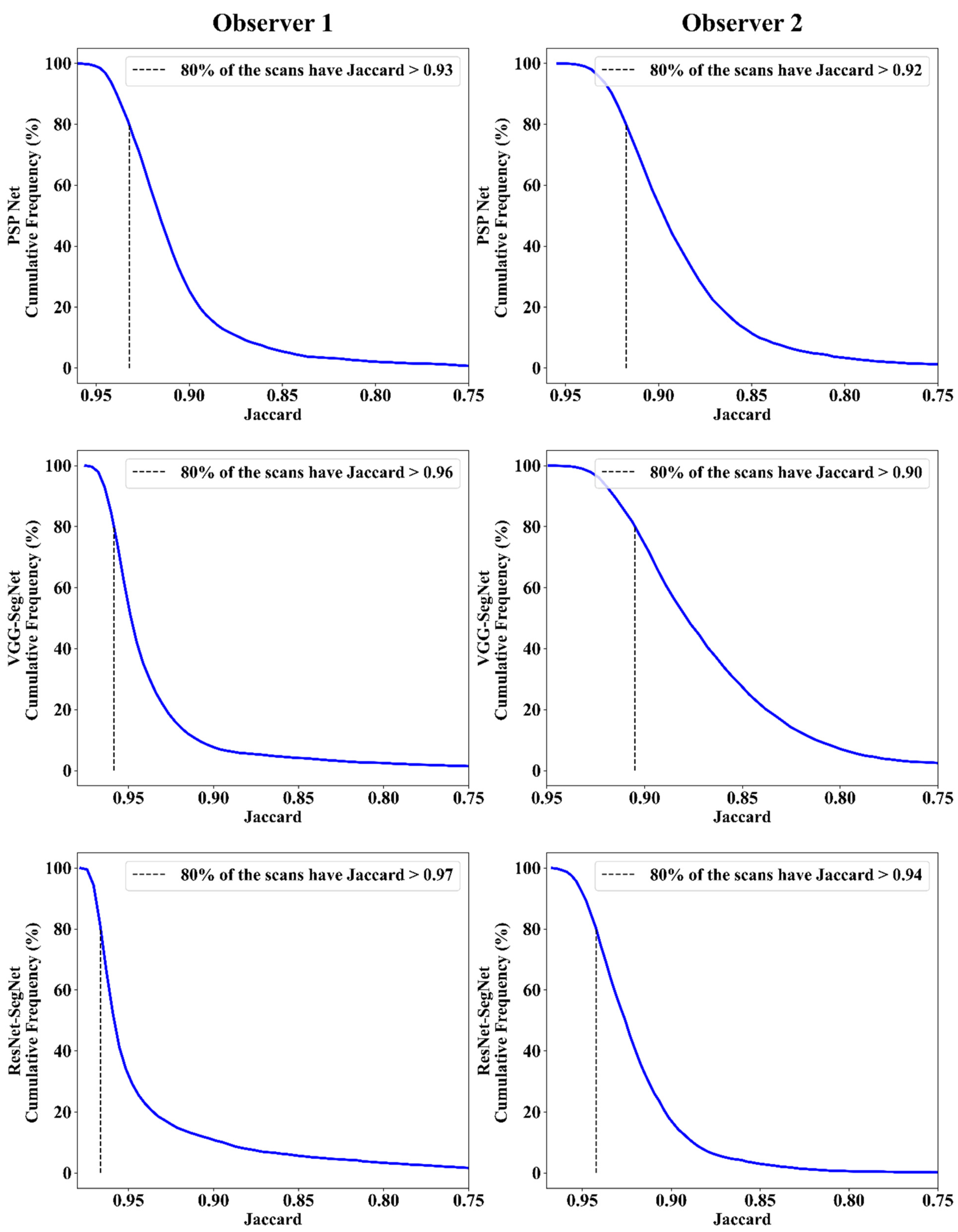
Jaccard Index and Dice Similarity
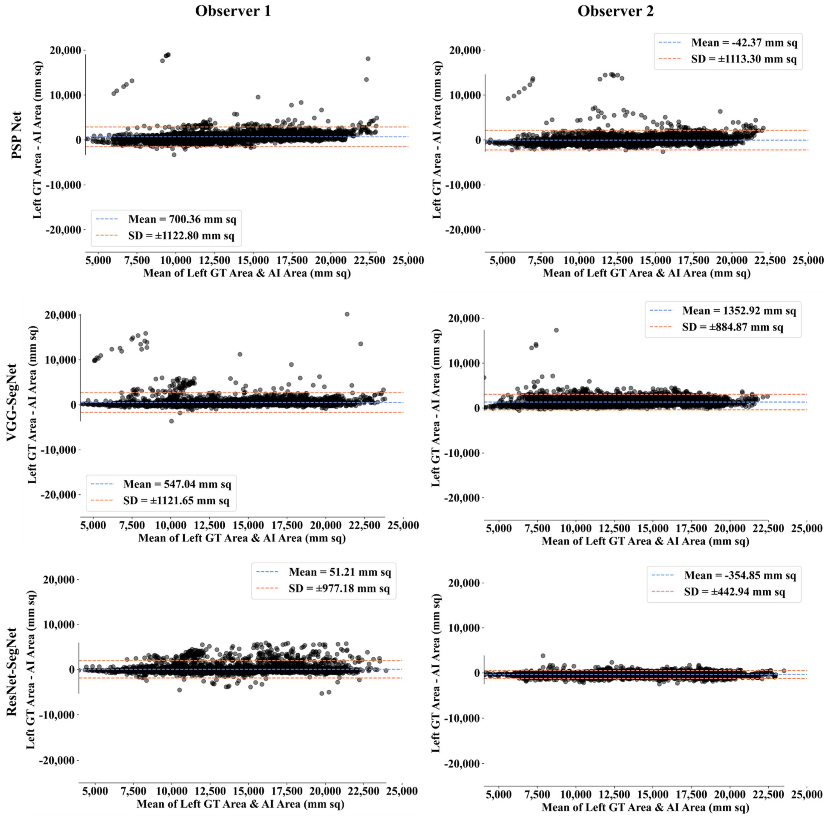
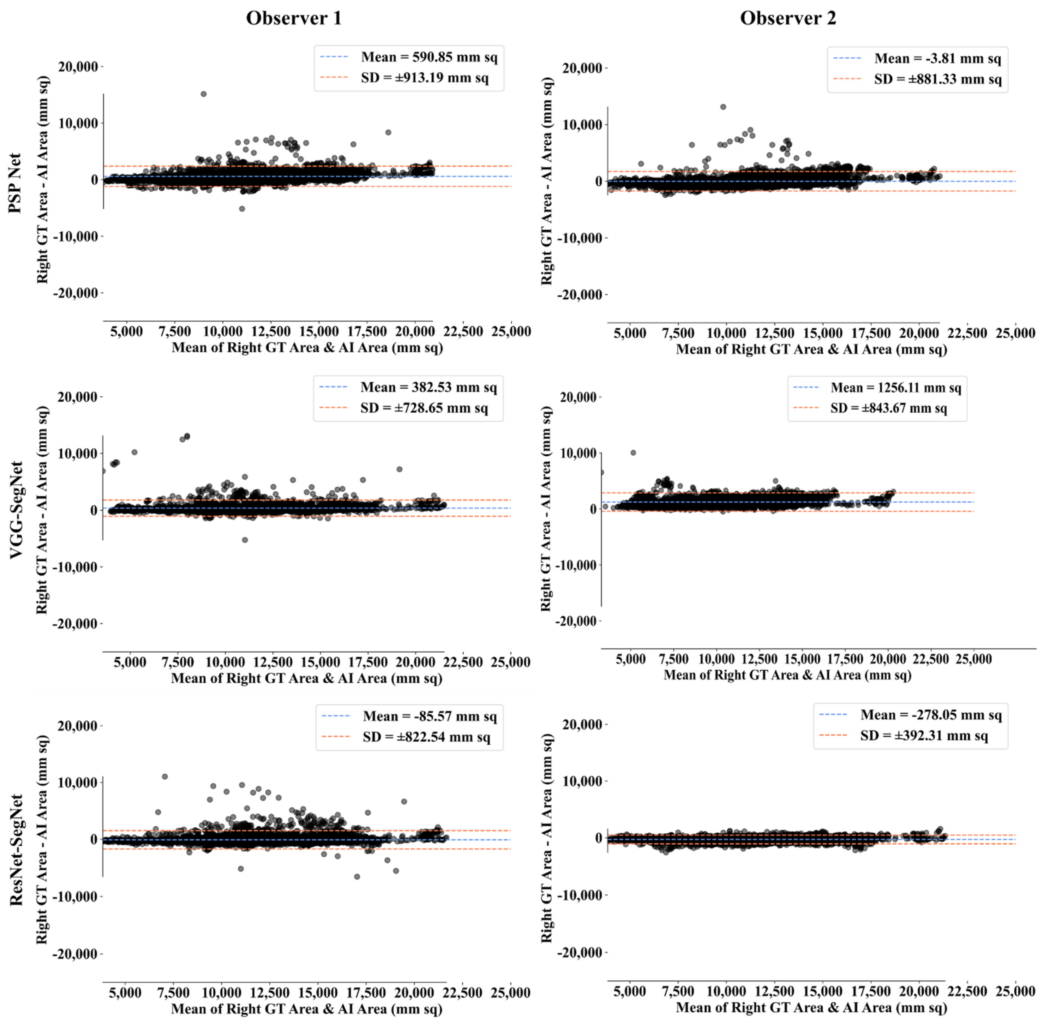
Bland-Altman Plot for Lung Area
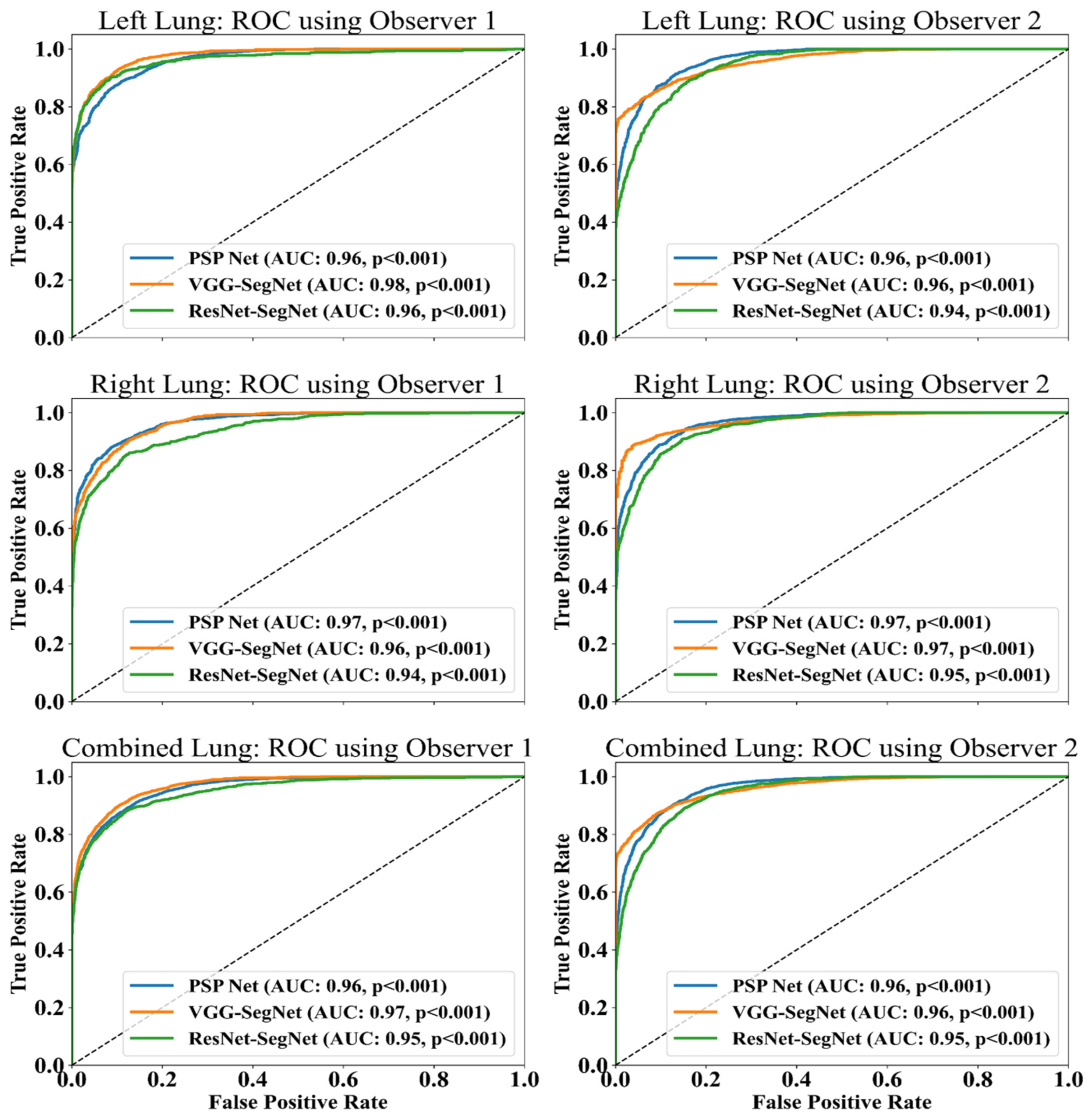
ROC Plots for Lung Area
4.2.3. Performance Evaluation Using Lung Long Axis Error
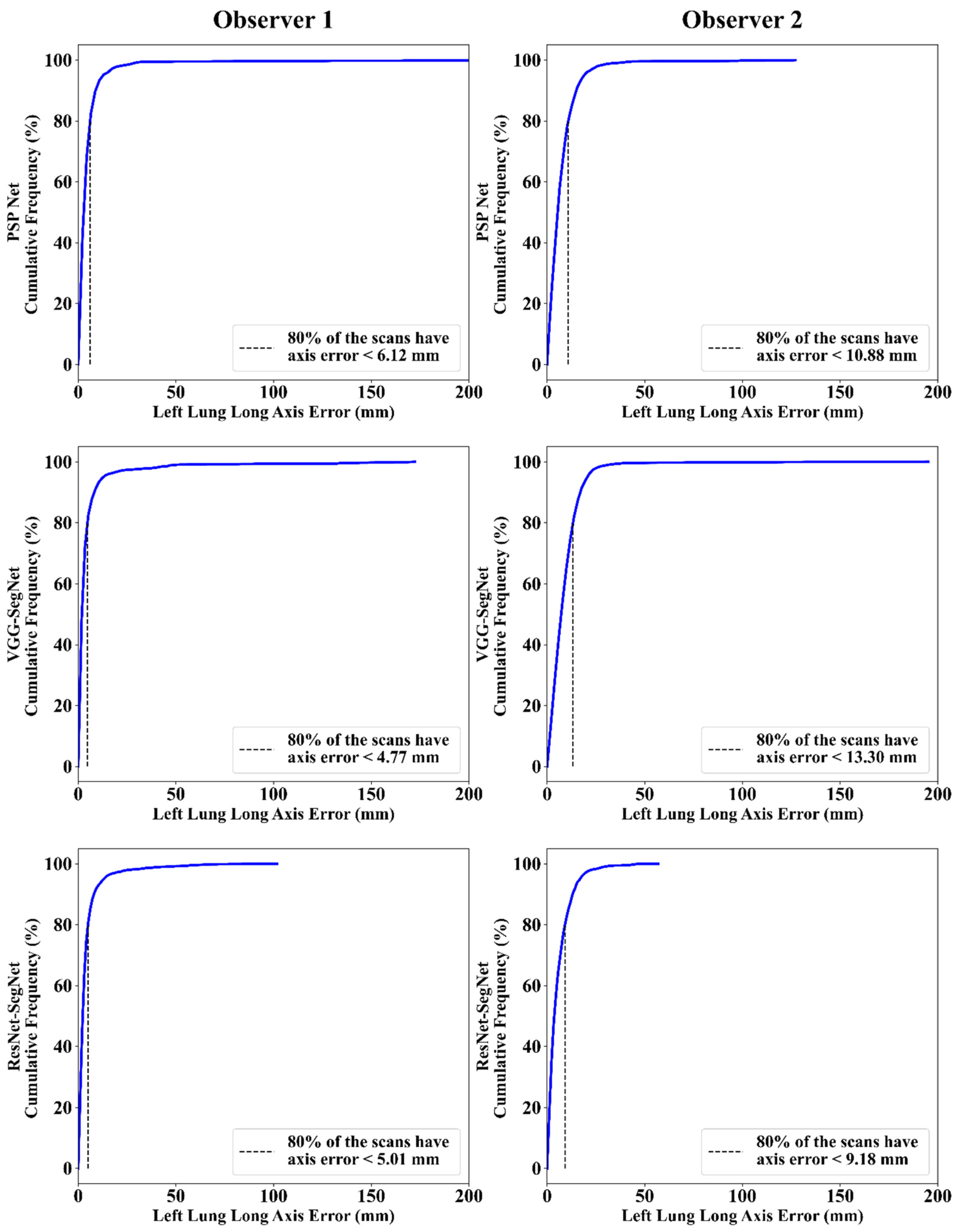
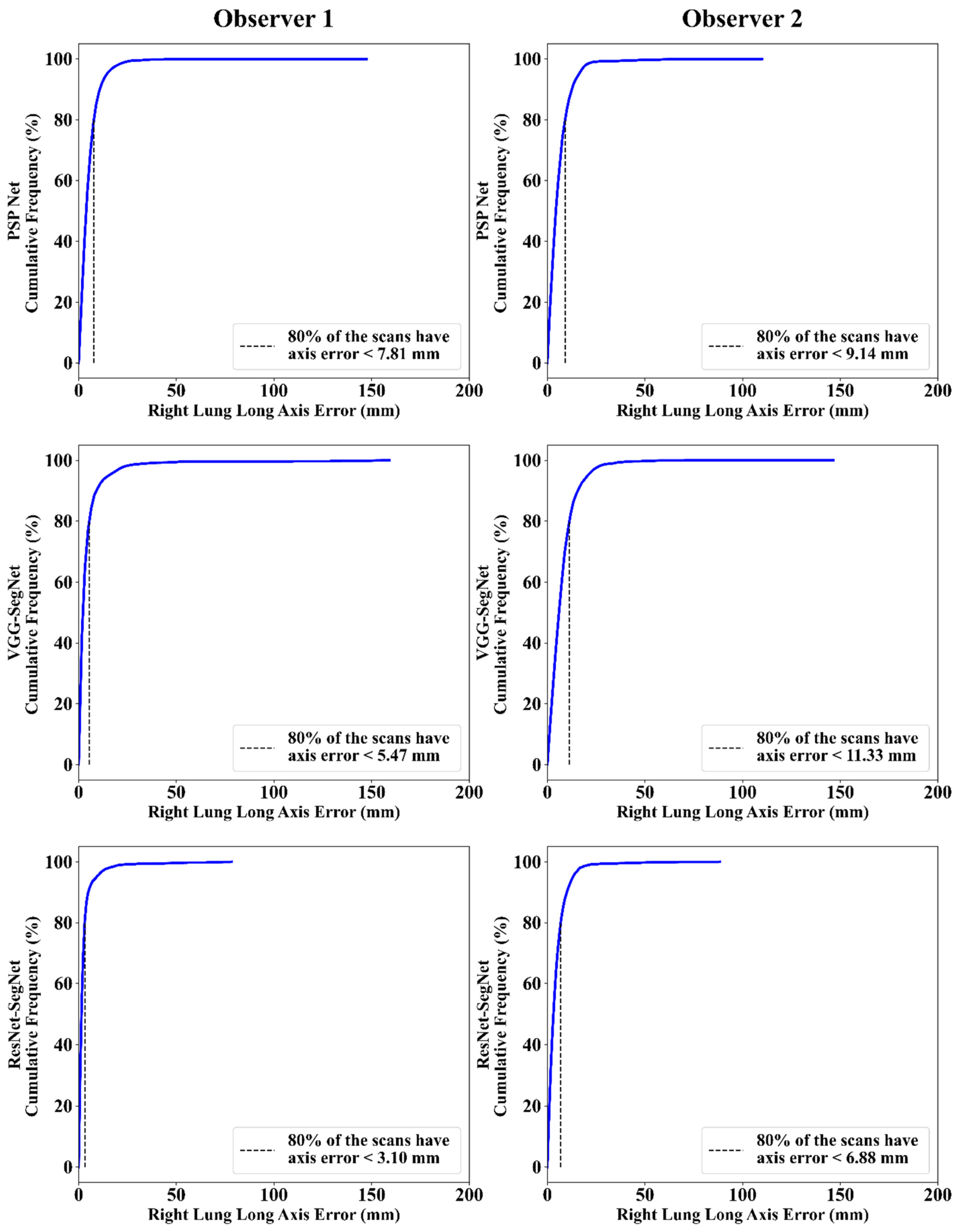
Cumulative Frequency Plot for Lung Long Axis Error
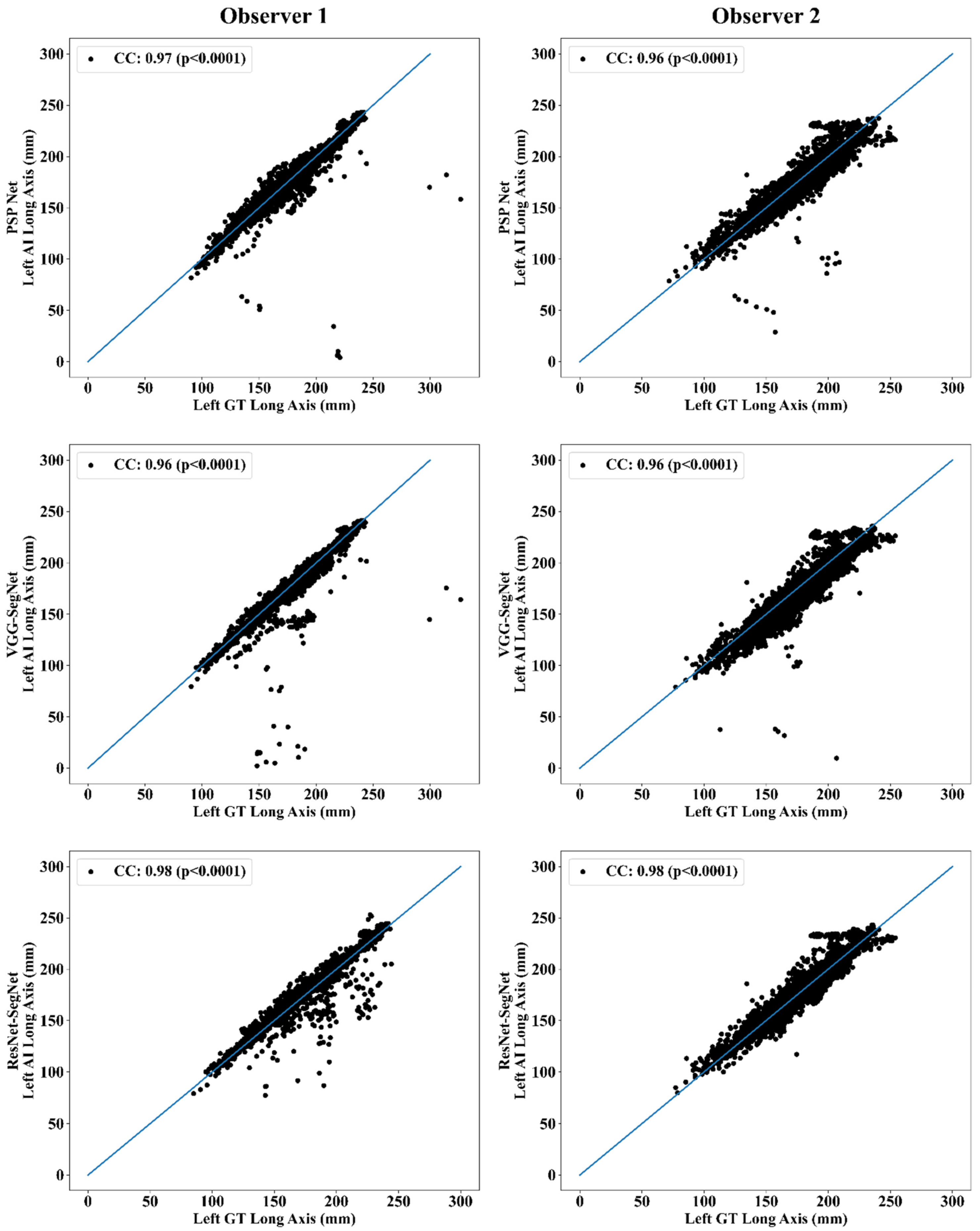
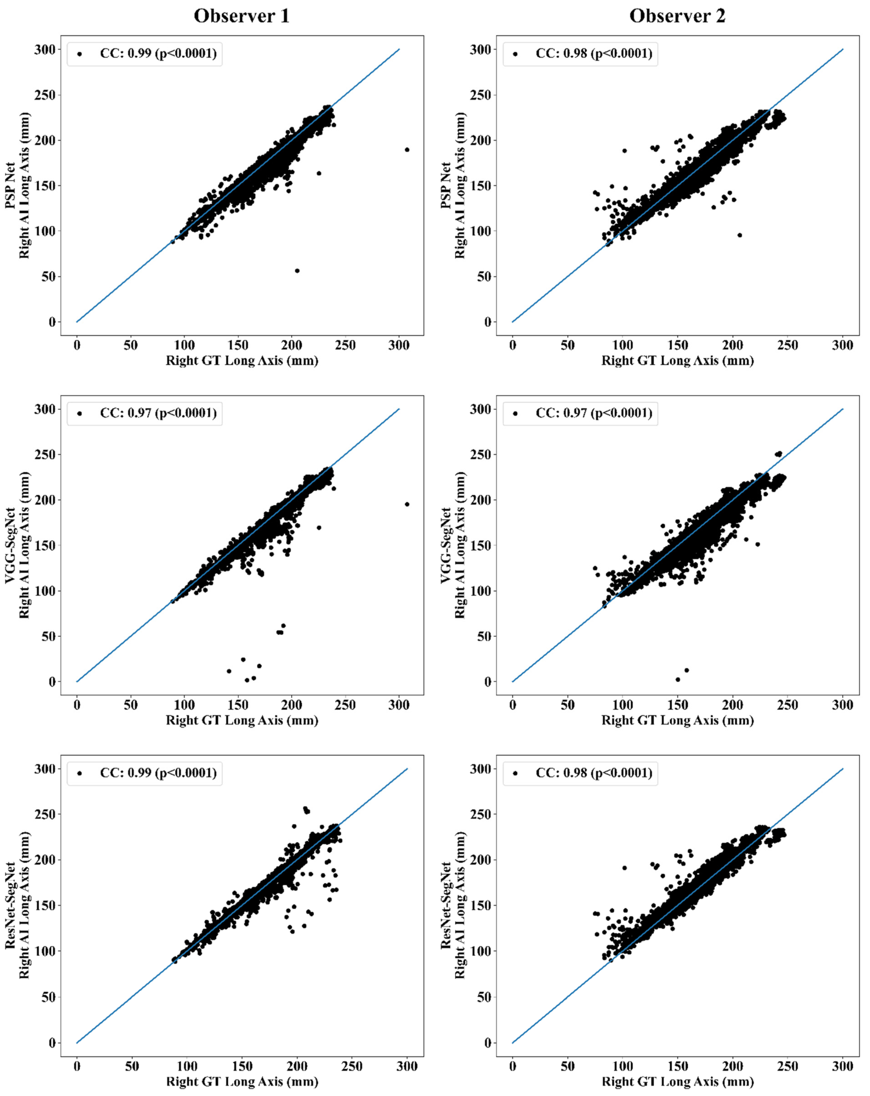
Correlation Plot for Lung Long Axis Error
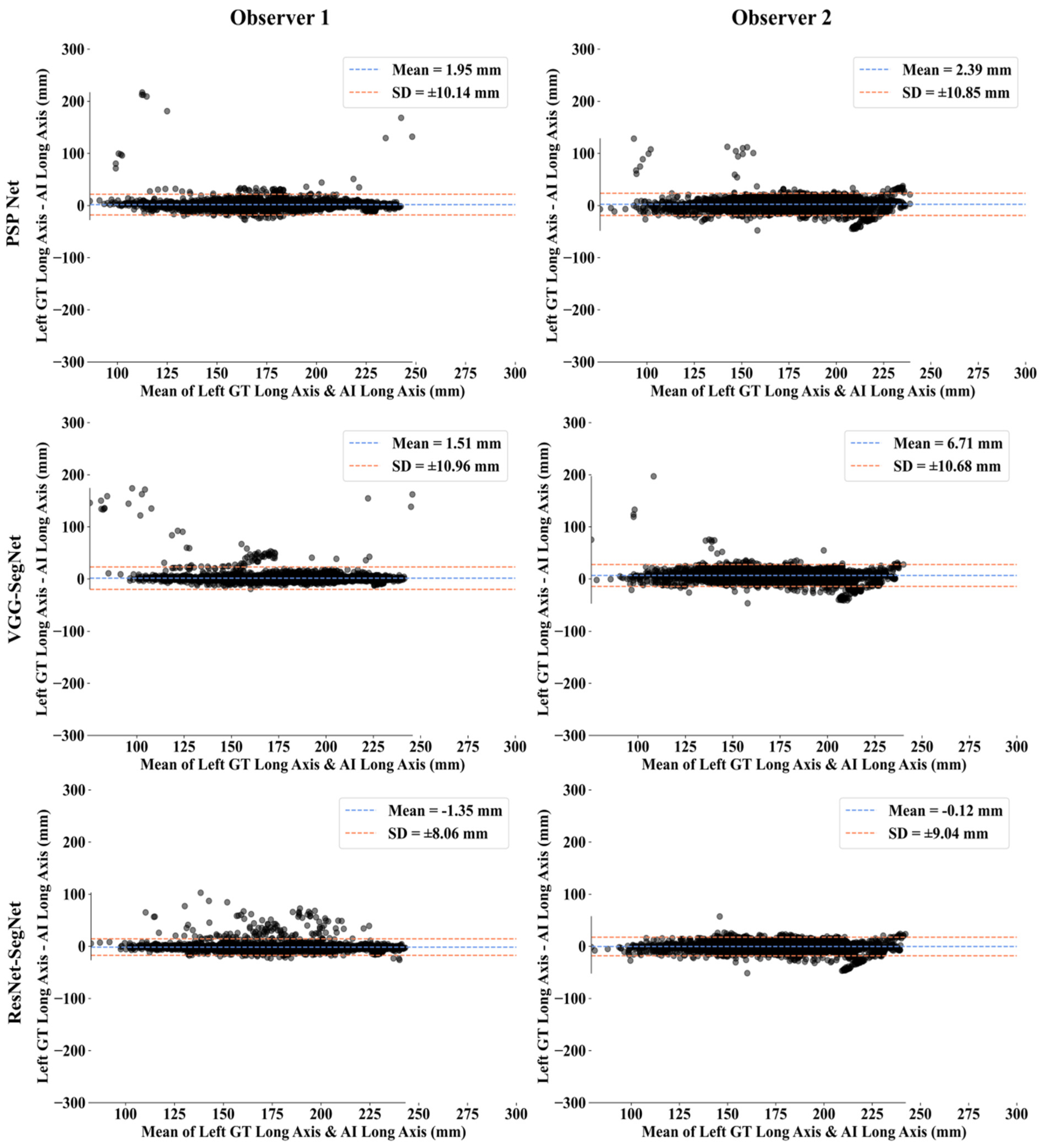
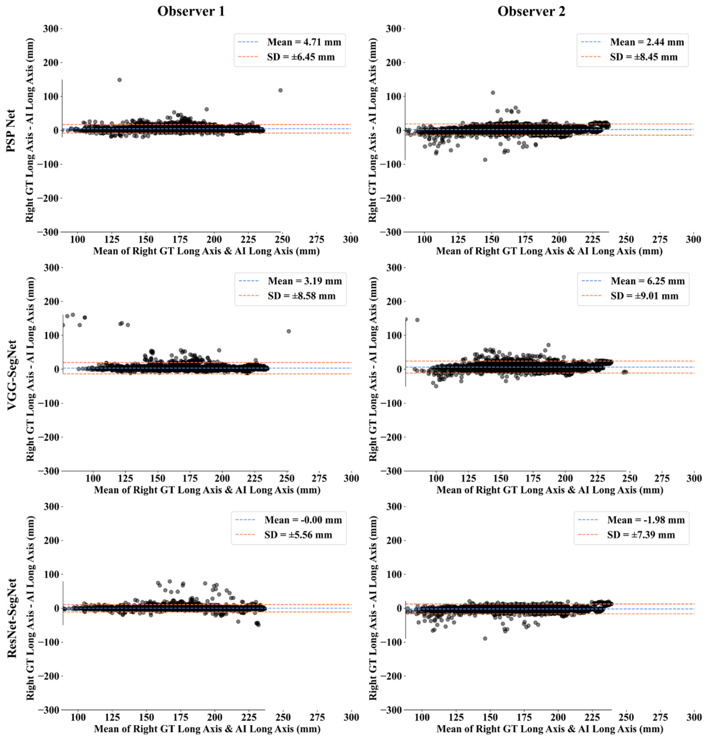
Bland-Altman Plots for Lung Long Axis Error
Statistical Tests
Figure of Merit
5. Discussion
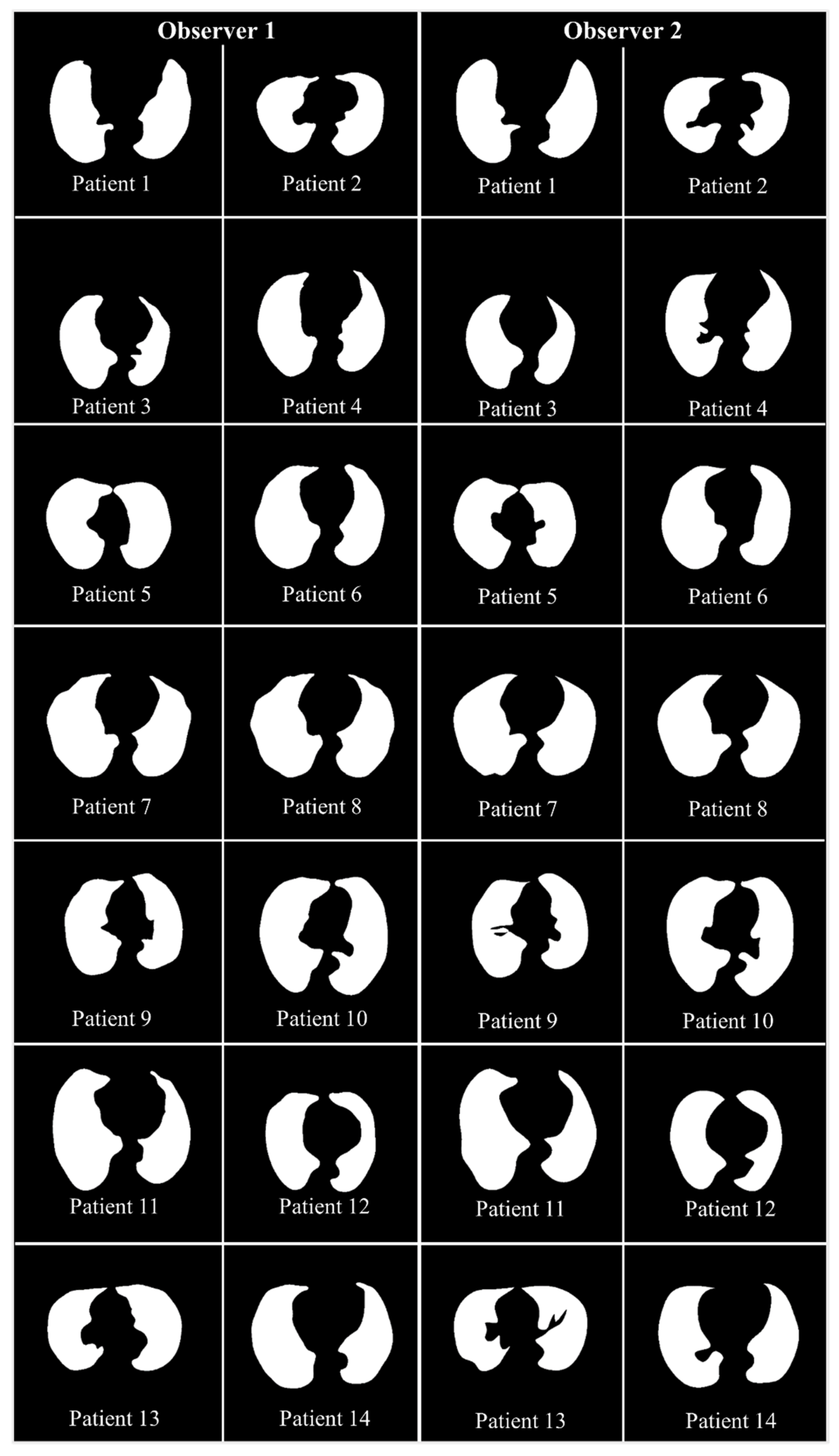
5.1. A Special Note on Three Model Behaviors with Respect to the Two OBSERVERS
5.2. Benchmarking
5.3. Strengths, Weakness, and Extensions
6. Conclusions
Author Contributions
Funding
Institutional Review Board Statement
Informed Consent Statement
Data Availability Statement
Conflicts of Interest
Abbreviations
| SN | Symbol | Description of the Symbols |
| 1 | ACC (ai) | Accuracy |
| 2 | AE | Area Error |
| 3 | AI | Artificial Intelligence |
| 4 | ARDS | Acute Respiratory Distress Syndrome |
| 5 | AUC | Area Under the Curve |
| 6 | BA | Bland-Altman |
| 7 | BE | Boundary Error |
| 8 | CC | Correlation coefficient |
| 9 | CE | Cross Entropy |
| 10 | COVID | Coronavirus disease |
| 11 | COVLIAS | COVID Lung Image Analysis System |
| 12 | CT | Computed Tomography |
| 13 | DL | Deep Learning |
| 14 | DS | Dice Similarity |
| 15 | FoM | Figure of merit |
| 16 | GT | Ground Truth |
| 17 | HDL | Hybrid Deep Learning |
| 18 | IS | Image Size |
| 19 | JI | Jaccard Index |
| 20 | LAE | Lung Area Error |
| 21 | LLAE | Lung Long Axis Error |
| 22 | NIH | National Institute of Health |
| 23 | PC | Pixel Counting |
| 24 | RF | Resolution Factor |
| 25 | ROC | Receiver operating characteristic |
| 26 | SDL | Solo Deep Learning |
| 27 | VGG | Visual Geometric Group |
| 28 | VS | Variability studies |
| 29 | WHO | World Health Organization |
Symbols
| SN | Symbol | Description of the Symbols |
| 1 | Cross Entropy-loss | |
| 2 | m | Model used for segmentation in the total number of models M |
| 3 | n | Image scan number in total number N |
| 4 | Mean estimated lung area for all images using AI model ‘m’ | |
| 5 | Estimated Lung Area using AI model ‘m’ and image ‘n’ | |
| 6 | GT lung area for image ‘n’ | |
| 7 | Mean ground truth area for all images N in the database | |
| 8 | Mean estimated lung long axis for all images using AI model ‘m’ | |
| 9 | Estimated lung long axis using AI model ‘m’ and image ‘n’ | |
| 10 | GT lung long axis for image ‘n’ | |
| 11 | Mean ground truth long axis for all images N in the database | |
| 12 | Figure-of-Merit for segmentation model ‘m’ | |
| 14 | Figure-of-Merit for long axis for model ‘m’ | |
| 15 | JI | Jaccard Index for a specific segmentation model |
| 16 | DSC | Dice Similarity Coefficient for a specific segmentation model |
| 17 | TP, TN | True Positive and True Negative |
| 18 | FP, FN | False Positive and False Negative |
| 19 | xi | GT label |
| 20 | pi | SoftMax classifier probability |
| 21 | Yp | Ground truth image |
| 22 | Estimated image | |
| 23 | P | Total no of pixels in an image in x, y-direction |
| 24 | K5 | Cross-validation protocol with 80% training and 20% testing (5 folds) |
| Deep Learning Segmentation Architectures | ||
| 25 | PSP Net | SDL model for lung segmentation with pyramidal feature extraction |
| 26 | VGG-SegNet | HDL model designed by fusion of VGG-19 and SegNet architecture |
| 27 | ResNet-SegNet | HDL model designed by fusion of ResNet-50 and SegNet architecture |
References
- Agarwal, M.; Saba, L.; Gupta, S.K.; Johri, A.M.; Khanna, N.N.; Mavrogeni, S.; Laird, J.R.; Pareek, G.; Miner, M.; Sfikakis, P.P. Wilson disease tissue classification and characterization using seven artificial intelligence models embedded with 3D optimization paradigm on a weak training brain magnetic resonance imaging datasets: A supercomputer application. Med. Biol. Eng. Comput. 2021, 59, 511–533. [Google Scholar] [CrossRef]
- Cau, R.; Pacielli, A.; Fatemeh, H.; Vaudano, P.; Arru, C.; Crivelli, P.; Stranieri, G.; Suri, J.S.; Mannelli, L.; Conti, M.; et al. Complications in COVID-19 patients: Characteristics of pulmonary embolism. Clin. Imaging 2021, 77, 244–249. [Google Scholar] [CrossRef] [PubMed]
- Saba, L.; Gerosa, C.; Fanni, D.; Marongiu, F.; La Nasa, G.; Caocci, G.; Barcellona, D.; Balestrieri, A.; Coghe, F.; Orru, G.; et al. Molecular pathways triggered by COVID-19 in different organs: ACE2 receptor-expressing cells under attack? A review. Eur. Rev. Med. Pharmacol. Sci. 2020, 24, 12609–12622. [Google Scholar]
- Cau, R.; Bassareo, P.P.; Mannelli, L.; Suri, J.S.; Saba, L. Imaging in COVID-19-related myocardial injury. Int. J. Cardiovasc. Imaging 2021, 37, 1349–1360. [Google Scholar] [CrossRef] [PubMed]
- Viswanathan, V.; Viswanathan, V.; Puvvula, A.; Jamthikar, A.D.; Saba, L.; Johri, A.M.; Kotsis, V.; Khanna, N.N.; Dhanjil, S.K.; Majhail, M.; et al. Bidirectional link between diabetes mellitus and coronavirus disease 2019 leading to cardiovascular disease: A narrative review. World J. Diabetes 2021, 12, 215–237. [Google Scholar] [CrossRef]
- Suri, J.S.; Agarwal, S.; Gupta, S.K.; Puvvula, A.; Biswas, M.; Saba, L.; Bit, A.; Tandel, G.S.; Agarwal, M.; Patrick, A.; et al. A narrative review on characterization of acute respiratory distress syndrome in COVID-19-infected lungs using artificial intelligence. Comput. Biol. Med. 2021, 130, 104210. [Google Scholar] [CrossRef]
- Cau, R.; Falaschi, Z.; Paschè, A.; Danna, P.; Arioli, R.; Arru, C.D.; Zagaria, D.; Tricca, S.; Suri, J.S.; Karla, M.K.; et al. Computed tomography findings of COVID-19 pneumonia in Intensive Care Unit-patients. J. Public Health Res. 2021, 10, 2270. [Google Scholar] [CrossRef]
- Emery, S.L.; Erdman, D.D.; Bowen, M.D.; Newton, B.R.; Winchell, J.M.; Meyer, R.F.; Tong, S.; Cook, B.T.; Holloway, B.P.; McCaustland, K.A.; et al. Real-time reverse transcription–polymerase chain reaction assay for SARS-associated coronavirus. Emerg. Infect. Dis. 2004, 10, 311–316. [Google Scholar] [CrossRef] [PubMed]
- Wu, X.; Hui, H.; Niu, M.; Li, L.; Wang, L.; He, B.; Yang, X.; Li, L.; Li, H.; Tian, J.; et al. Deep learning-based multi-view fusion model for screening 2019 novel coronavirus pneumonia: A multicentre study. Eur. J. Radiol. 2020, 128, 109041. [Google Scholar] [CrossRef] [PubMed]
- Pathak, Y.; Shukla, P.K.; Tiwari, A.; Stalin, S.; Singh, S. Deep transfer learning based classification model for COVID-19 disease. IRBM 2020, in press. [Google Scholar] [CrossRef]
- Saba, L.; Suri, J.S. Multi-Detector CT Imaging: Principles, Head, Neck, and Vascular Systems; CRC Press: Boca Raton, FL, USA, 2013; Volume 1. [Google Scholar]
- Gozes, O.; Frid-Adar, M.; Greenspan, H.; Browning, P.D.; Zhang, H.; Ji, W.; Bernheim, A.; Siegel, E. Rapid ai development cycle for the coronavirus (COVID-19) pandemic: Initial results for automated detection & patient monitoring using deep learning ct image analysis. arXiv 2020, arXiv:05037. [Google Scholar]
- Shalbaf, A.; Vafaeezadeh, M. Automated detection of COVID-19 using ensemble of transfer learning with deep convolutional neural network based on CT scans. Int. J. Comput. Assist. Radiol. Surg. 2021, 16, 115–123. [Google Scholar]
- Yang, X.; He, X.; Zhao, J.; Zhang, Y.; Zhang, S.; Xie, P. COVID-CT-dataset: A CT scan dataset about COVID-19. arXiv 2020, arXiv:13865. [Google Scholar]
- Alqudah, A.M.; Qazan, S.; Alquran, H.; Qasmieh, I.A.; Alqudah, A. COVID-2019 Detection Using X-ray Images and Artificial Intelligence Hybrid Systems. Phys. Sci. 2020, 2, 1. [Google Scholar]
- Aslan, M.F.; Unlersen, M.F.; Sabanci, K.; Durdu, A. CNN-based transfer learning–BiLSTM network: A novel approach for COVID-19 infection detection. Appl. Soft Comput. 2021, 98, 10691. [Google Scholar] [CrossRef]
- Wu, Y.H.; Gao, S.H.; Mei, J.; Xu, J.; Fan, D.P.; Zhang, R.G.; Cheng, M.M. Jcs: An explainable COVID-19 diagnosis system by joint classification and segmentation. IEEE Trans. Image Process. 2021, 30, 3113–3126. [Google Scholar] [CrossRef] [PubMed]
- Xu, X.; Jiang, X.; Ma, C.; Du, P.; Li, X.; Lv, S.; Yu, L.; Ni, Q.; Chen, Y.; Su, J.; et al. A deep learning system to screen novel coronavirus disease 2019 pneumonia. Engineering 2020, 6, 1122–1129. [Google Scholar] [CrossRef] [PubMed]
- El-Baz, A.; Suri, J. Machine Learning in Medicine; CRC Press: Boca Raton, FL, USA, 2021; ISBN 9781138106901. [Google Scholar]
- Suri, J.S.; Rangayyan, R.M. Recent Advances in Breast Imaging, Mammography, and Computer-Aided Diagnosis of Breast Cancer; SPIE Publications: Bellingham, WA, USA, 2006. [Google Scholar]
- Biswas, M.; Kuppili, V.; Edla, D.R.; Suri, H.S.; Saba, L.; Marinhoe, R.T.; Sanches, J.M.; Suri, J.S. Symtosis: A liver ultrasound tissue characterization and risk stratification in optimized deep learning paradigm. Comput. Methods Programs Biomed. 2018, 155, 165–177. [Google Scholar] [CrossRef] [PubMed]
- Acharya, U.R.; Sree, S.V.; Ribeiro, R.; Krishnamurthi, G.; Marinho, R.T.; Sanches, J.; Suri, J.S. Data mining framework for fatty liver disease classification in ultrasound: A hybrid feature extraction paradigm. Med. Phys. 2012, 39, 4255–4264. [Google Scholar] [CrossRef] [PubMed] [Green Version]
- Acharya, U.R.; Sree, S.V.; Krishnan, M.M.R.; Molinari, F.; Garberoglio, R.; Suri, J.S. Non-invasive automated 3D thyroid lesion classification in ultrasound: A class of ThyroScan™ systems. Ultrasonics 2012, 52, 508–520. [Google Scholar] [CrossRef]
- Acharya, U.R.; Swapna, G.; Sree, S.V.; Molinari, F.; Gupta, S.; Bardales, R.H.; Witkowska, A.; Suri, J.S. A review on ultrasound-based thyroid cancer tissue characterization and automated classification. Technol. Cancer Res. Treat. 2014, 13, 289–301. [Google Scholar] [CrossRef] [Green Version]
- Molinari, F.; Mantovani, A.; Deandrea, M.; Limone, P.; Garberoglio, R.; Suri, J.S. Characterization of single thyroid nodules by contrast-enhanced 3-D ultrasound. Ultrasound Med. Biol. 2010, 36, 1616–1625. [Google Scholar] [CrossRef] [Green Version]
- Shrivastava, V.K.; Londhe, N.D.; Sonawane, R.S.; Suri, J.S. Computer-aided diagnosis of psoriasis skin images with HOS, texture and color features: A first comparative study of its kind. Comput. Methods Programs Biomed. 2016, 126, 98–109. [Google Scholar] [CrossRef] [PubMed]
- Shrivastava, V.K.; Londhe, N.D.; Sonawane, R.S.; Suri, J.S. Reliable and accurate psoriasis disease classification in dermatology images using comprehensive feature space in machine learning paradigm. Expert Syst. Appl. 2015, 42, 6184–6195. [Google Scholar] [CrossRef]
- Pareek, G.; Acharya, U.R.; Sree, S.V.; Swapna, G.; Yantri, R.; Martis, R.J.; Saba, L.; Krishnamurthi, G.; Mallarini, G.; El-Baz, A.; et al. Prostate tissue characterization/classification in 144 patient population using wavelet and higher order spectra features from transrectal ultrasound images. Technol. Cancer Res. Treat. 2013, 12, 545–557. [Google Scholar] [CrossRef]
- McClure, P.; Elnakib, A.; El-Ghar, M.A.; Khalifa, F.; Soliman, A.; El-Diasty, T.; Suri, J.S.; Elmaghraby, A.; El-Baz, A. In-vitro and in-vivo diagnostic techniques for prostate cancer: A review. J. Biomed. Nanotechnol. 2014, 10, 2747–2777. [Google Scholar] [CrossRef] [PubMed]
- Mookiah, M.R.K.; Acharya, U.R.; Martis, R.J.; Chua, C.K.; Lim, C.M.; Ng, E.Y.K.; Laude, A. Evolutionary algorithm based classifier parameter tuning for automatic diabetic retinopathy grading: A hybrid feature extraction approach. Knowl.-Based Syst. 2013, 39, 9–22. [Google Scholar] [CrossRef]
- Than, J.C.; Saba, L.; Noor, N.M.; Rijal, O.M.; Kassim, R.M.; Yunus, A.; Suri, H.S.; Porcu, M.; Suri, J.S. Lung disease stratification using amalgamation of Riesz and Gabor transforms in machine learning framework. Comput. Biol. Med. 2017, 89, 197–211. [Google Scholar] [CrossRef] [PubMed]
- El-Baz, A.; Jiang, X.; Suri, J.S. Biomedical Image Segmentation: Advances and Trends; CRC Press: Boca Raton, FL, USA, 2016. [Google Scholar]
- Than, J.C.; Saba, L.; Noor, N.M.; Rijal, O.M.; Kassim, R.M.; Yunus, A.; Suri, H.S.; Porcu, M.; Suri, J.S. Shape recovery algorithms using level sets in 2-D/3-D medical imagery: A state-of-the-art review. IEEE Trans. Inf. Technol. Biomed. 2002, 6, 8–28. [Google Scholar]
- El-Baz, A.S.; Acharya, R.; Mirmehdi, M.; Suri, J.S. Multi Modality State-of-the-Art Medical Image Segmentation and Registration Methodologies; Springer Science & Business Media: Berlin, Germany, 2011; Volume 2. [Google Scholar]
- El-Baz, A.; Suri, J.S. Level Set Method in Medical Imaging Segmentation; CRC Press: Boca Raton, FL, USA, 2019. [Google Scholar]
- Saba, L.; Sanagala, S.S.; Gupta, S.K.; Koppula, V.K.; Johri, A.M.; Khanna, N.N.; Mavrogeni, S.; Laird, J.R.; Pareek, G.; Miner, M.; et al. Multimodality carotid plaque tissue characterization and classification in the artificial intelligence paradigm: A narrative review for stroke application. Ann. Transl. Med. 2021, 9, 1206. [Google Scholar] [CrossRef] [PubMed]
- Acharya, U.R.; Sree, S.V.; Krishnan, M.M.R.; Krishnananda, N.; Ranjan, S.; Umesh, P.; Suri, J.S. Automated classification of patients with coronary artery disease using grayscale features from left ventricle echocardiographic images. Comput. Methods Programs Biomed. 2013, 112, 624–632. [Google Scholar] [CrossRef]
- Agarwal, M.; Saba, L.; Gupta, S.K.; Carriero, A.; Falaschi, Z.; Paschè, A.; Danna, P.; El-Baz, A.; Naidu, S.; Suri, J.S. A novel block imaging technique using nine artificial intelligence models for COVID-19 disease classification, characterization and severity measurement in lung computed tomography scans on an Italian cohort. J. Med. Syst. 2021, 45, 1–30. [Google Scholar] [CrossRef]
- Saba, L.; Agarwal, M.; Patrick, A.; Puvvula, A.; Gupta, S.K.; Carriero, A.; Laird, J.R.; Kitas, G.D.; Johri, A.M.; Balestrieri, A.; et al. Six artificial intelligence paradigms for tissue characterisation and classification of non-COVID-19 pneumonia against COVID-19 pneumonia in computed tomography lungs. Int. J. Comput. Assist. Radiol. Surg. 2021, 16, 423–434. [Google Scholar] [CrossRef]
- Skandha, S.S.; Gupta, S.K.; Saba, L.; Koppula, V.K.; Johri, A.M.; Khanna, N.N.; Mavrogeni, S.; Laird, J.R.; Pareek, G.; Miner, M.; et al. 3-D optimized classification and characterization artificial intelligence paradigm for cardiovascular/stroke risk stratification using carotid ultrasound-based delineated plaque: Atheromatic™ 2.0. Comput. Biol. Med. 2020, 125, 103958. [Google Scholar] [CrossRef]
- Tandel, G.S.; Balestrieri, A.; Jujaray, T.; Khanna, N.N.; Saba, L.; Suri, J.S. Multiclass magnetic resonance imaging brain tumor classification using artificial intelligence paradigm. Comput. Biol. Med. 2020, 122, 103804. [Google Scholar] [CrossRef] [PubMed]
- Sarker, M.M.K.; Makhlouf, Y.; Banu, S.F.; Chambon, S.; Radeva, P.; Puig, D. Web-based efficient dual attention networks to detect COVID-19 from X-ray images. Electron. Lett. 2020, 56, 1298–1301. [Google Scholar] [CrossRef]
- Sarker, M.M.K.; Makhlouf, Y.; Craig, S.G.; Humphries, M.P.; Loughrey, M.; James, J.A.; Salto-Tellez, M.; O’Reilly, P.; Maxwell, P. A Means of Assessing Deep Learning-Based Detection of ICOS Protein Expression in Colon Cancer. Cancers 2021, 13, 3825. [Google Scholar] [CrossRef] [PubMed]
- Jain, P.K.; Sharma, N.; Giannopoulos, A.A.; Saba, L.; Nicolaides, A.; Suri, J.S. Hybrid deep learning segmentation models for atherosclerotic plaque in internal carotid artery B-mode ultrasound. Comput. Biol. Med. 2021, 136, 104721. [Google Scholar] [CrossRef]
- Jena, B.; Saxena, S.; Nayak, G.K.; Saba, L.; Sharma, N.; Suri, J.S. Artificial Intelligence-based Hybrid Deep Learning Models for Image Classification: The First Narrative Review. Comput. Biol. Med. 2021, 137, 104803. [Google Scholar] [CrossRef] [PubMed]
- Suri, J.; Agarwal, S.; Gupta, S.K.; Puvvula, A.; Viskovic, K.; Suri, N.; Alizad, A.; El-Baz, A.; Saba, L.; Fatemi, M.; et al. Systematic Review of Artificial Intelligence in Acute Respiratory Distress Syndrome for COVID-19 Lung Patients: A Biomedical Imaging Perspective. IEEE J. Biomed. Health Inform. 2021, 25. [Google Scholar]
- Saba, L.; Banchhor, S.K.; Araki, T.; Viskovic, K.; Londhe, N.D.; Laird, J.R.; Suri, H.S.; Suri, J.S. Intra- and inter-operator reproducibility of automated cloud-based carotid lumen diameter ultrasound measurement. Indian Heart J. 2018, 70, 649–664. [Google Scholar] [CrossRef] [PubMed]
- Saba, L.; Than, J.C.; Noor, N.M.; Rijal, O.M.; Kassim, R.M.; Yunus, A.; Ng, C.R.; Suri, J.S. Inter-observer Variability Analysis of Automatic Lung Delineation in Normal and Disease Patients. J. Med. Syst. 2016, 40, 142. [Google Scholar] [CrossRef]
- Zhang, S.; Suri, J.S.; Salvado, O.; Chen, Y.; Wacker, F.K.; Wilson, D.L.; Duerk, J.L.; Lewin, J.S. Inter-and Intra-Observer Variability Assessment of in Vivo Carotid Plaque Burden Quantification Using Multi-Contrast Dark Blood MR Images. Stud. Health Technol. Inform. 2005, 113, 384–393. [Google Scholar] [PubMed]
- Aggarwal, D.; Saini, V. Factors limiting the utility of bronchoalveolar lavage in the diagnosis of COVID-19. Eur. Respir. J. 2020, 56, 2003116. [Google Scholar] [CrossRef]
- Saba, L.; Banchhor, S.K.; Suri, H.S.; Londhe, N.D.; Araki, T.; Ikeda, N.; Viskovic, K.; Shafique, S.; Laird, J.R.; Gupta, A.; et al. Accurate cloud-based smart IMT measurement, its validation and stroke risk stratification in carotid ultrasound: A web-based point-of-care tool for multicenter clinical trial. Comput. Biol. Med. 2016, 75, 217–234. [Google Scholar] [CrossRef]
- Zhao, H.; Shi, J.; Qi, X.; Wang, X.; Jia, J. Pyramid scene parsing network. In Proceedings of the IEEE Conference on Computer Vision and Pattern Recognition, Honolulu, HI, USA, 21–26 July 2017; pp. 2881–2890. [Google Scholar]
- Simonyan, K.; Zisserman, A. Very deep convolutional networks for large-scale image recognition. arXiv 2014, arXiv:1409.1556. [Google Scholar]
- Suri, J.S.; Agarwal, S.; Pathak, R.; Ketireddy, V.; Columbu, M.; Saba, L.; Gupta, S.K.; Faa, G.; Singh, I.M.; Turk, M.; et al. COVLIAS 1.0: Lung Segmentation in COVID-19 Computed Tomography Scans Using Hybrid Deep Learning Artificial Intelligence Models. Diagnostics 2021, 11, 1405. [Google Scholar] [CrossRef] [PubMed]
- He, K.; Zhang, X.; Ren, S.; Sun, J. Deep residual learning for image recognition. In Proceedings of the IEEE Conference on Computer Vision and Pattern Recognition, Las Vegas, NV, USA, 27–30 June 2016; IEEE: Piscataway, NJ, USA, 2016; pp. 770–778. [Google Scholar]
- Acharya, U.R.; Faust, O.; Sree, S.V.; Molinari, F.; Saba, L.; Nicolaides, A.; Suri, J.S. An accurate and generalized approach to plaque characterization in 346 carotid ultrasound scans. IEEE Trans. Instrum. Meas. 2012, 61, 1045–1053. [Google Scholar] [CrossRef]
- Acharya, U.R.; Saba, L.; Molinari, F.; Guerriero, S.; Suri, J.S. Ovarian tumor characterization and classification: A class of GyneScan™ systems. In Proceedings of the 2012 Annual International Conference of the IEEE Engineering in Medicine and Biology Society, San Diego, CA, USA, 28 August–1 September 2012; IEEE: Piscataway, NJ, USA, 2012. [Google Scholar]
- Araki, T.; Ikeda, N.; Dey, N.; Acharjee, S.; Molinari, F.; Saba, L.; Godia, E.C.; Nicolaides, A.; Suri, J.S. Shape-based approach for coronary calcium lesion volume measurement on intravascular ultrasound imaging and its association with carotid intima-media thickness. J. Ultrasound Med. 2015, 34, 469–482. [Google Scholar] [CrossRef]
- Barqawi, A.B.; Li, L.; Crawford, E.D.; Fenster, A.; Werahera, P.N.; Kumar, D.; Miller, S.; Suri, J.S. Three different strategies for real-time prostate capsule volume computation from 3-D end-fire transrectal ultrasound. In Proceedings of the 2007 29th Annual International Conference of the IEEE Engineering in Medicine and Biology Society, Lyon, France, 22–26 August 2007; IEEE: Piscataway, NJ, USA, 2007. [Google Scholar]
- Suri, J.S.; Haralick, R.M.; Sheehan, F.H. Left ventricle longitudinal axis fitting and its apex estimation using a robust algorithm and its performance: A parametric apex model. In Proceedings of the International Conference on Image Processing, Santa Barbara, CA, USA, 14–17 July 1997; IEEE: Piscataway, NJ, USA, 1997. [Google Scholar]
- Singh, B.K.; Verma, K.; Thoke, A.S.; Suri, J.S. Risk stratification of 2D ultrasound-based breast lesions using hybrid feature selection in machine learning paradigm. Measurement 2017, 105, 146–157. [Google Scholar] [CrossRef]
- Riffenburgh, R.H.; Gillen, D.L. Contents. In Statistics in Medicine; Academic Press: Cambridge, MA, USA, 2020; pp. ix–xvi. [Google Scholar]
- Acharya, R.U.; Faust, O.; Alvin, A.P.C.; Sree, S.V.; Molinari, F.; Saba, L.; Nicolaides, A.; Suri, J.S. Symptomatic vs. asymptomatic plaque classification in carotid ultrasound. J. Med. Syst. 2012, 36, 1861–1871. [Google Scholar] [CrossRef]
- Acharya, U.R.; Vinitha Sree, S.; Mookiah, M.R.K.; Yantri, R.; Molinari, F.; Zieleźnik, W.; Małyszek-Tumidajewicz, J.; Stępień, B.; Bardales, R.H.; Witkowska, A.; et al. Diagnosis of Hashimoto’s thyroiditis in ultrasound using tissue characterization and pixel classification. Proc. Inst. Mech. Eng. Part H J. Eng. Med. 2013, 227, 788–798. [Google Scholar] [CrossRef]
- Acharya, U.R.; Faust, O.; Alvin, A.P.C.; Krishnamurthi, G.; Seabra, J.C.; Sanches, J.; Suri, J.S. Understanding symptomatology of atherosclerotic plaque by image-based tissue characterization. Comput. Methods Programs Biomed. 2013, 110, 66–75. [Google Scholar] [CrossRef]
- Acharya, U.R.; Faust, O.; Sree, S.V.; Alvin, A.P.C.; Krishnamurthi, G.; Sanches, J.; Suri, J.S. Atheromatic™: Symptomatic vs. asymptomatic classification of carotid ultrasound plaque using a combination of HOS, DWT & texture. In Proceedings of the 2011 Annual International Conference of the IEEE Engineering in Medicine and Biology Society, Boston, MA, USA, 3 August–3 September 2011; IEEE: Piscataway, NJ, USA, 2011. [Google Scholar]
- Acharya, U.R.; Mookiah, M.R.K.; Sree, S.V.; Afonso, D.; Sanches, J.; Shafique, S.; Nicolaides, A.; Pedro, L.M.; e Fernandes, J.F.; Suri, J.S. Atherosclerotic plaque tissue characterization in 2D ultrasound longitudinal carotid scans for automated classification: A paradigm for stroke risk assessment. Med. Biol. Eng. Comput. 2013, 51, 513–523. [Google Scholar] [CrossRef]
- Molinari, F.; Liboni, W.; Pavanelli, E.; Giustetto, P.; Badalamenti, S.; Suri, J.S. Accurate and automatic carotid plaque characterization in contrast enhanced 2-D ultrasound images. In Proceedings of the 29th Annual International Conference of the IEEE Engineering in Medicine and Biology Society, Lyon, France, 22–26 August 2007; IEEE: Piscataway, NJ, USA, 2007. [Google Scholar]
- Saba, L.; Biswas, M.; Suri, H.S.; Viskovic, K.; Laird, J.R.; Cuadrado-Godia, E.; Nicolaides, A.; Khanna, N.N.; Viswanathan, V.; Suri, J.S. Ultrasound-based carotid stenosis measurement and risk stratification in diabetic cohort: A deep learning paradigm. Cardiovasc. Diagn. Ther. 2019, 9, 439–461. [Google Scholar] [CrossRef]
- Biswas, M.; Kuppili, V.; Saba, L.; Edla, D.R.; Suri, H.S.; Sharma, A.; Cuadrado-Godia, E.; Laird, J.R.; Nicolaides, A.; Suri, J.S. Deep learning fully convolution network for lumen characterization in diabetic patients using carotid ultrasound: A tool for stroke risk. Med Biol. Eng. Comput. 2019, 57, 543–564. [Google Scholar] [CrossRef]
- Chaddad, A.; Hassan, L.; Desrosiers, C. Deep CNN models for predicting COVID-19 in CT and x-ray images. J. Med. Imaging 2021, 8 (Suppl. S1), 014502. [Google Scholar] [CrossRef] [PubMed]
- Gunraj, H.; Wang, L.; Wong, A. COVIDNet-CT: A Tailored Deep Convolutional Neural Network Design for Detection of COVID-19 Cases From Chest CT Images. Front. Med. 2020, 7, 608525. [Google Scholar] [CrossRef] [PubMed]
- Iyer, T.J.; Raj, A.N.J.; Ghildiyal, S.; Nersisson, R. Performance analysis of lightweight CNN models to segment infectious lung tissues of COVID-19 cases from tomographic images. PeerJ Comput. Sci. 2021, 7, e368. [Google Scholar] [CrossRef]
- Ranjbarzadeh, R.; Jafarzadeh Ghoushchi, S.; Bendechache, M.; Amirabadi, A.; Ab Rahman, M.N.; Baseri Saadi, S.; Aghamohammadi, A.; Kooshki Forooshani, M. Lung Infection Segmentation for COVID-19 Pneumonia Based on a Cascade Convolutional Network from CT Images. BioMed Res. Int. 2021, 2021, 5544742. [Google Scholar] [CrossRef]
- Erasmus, J.J.; Gladish, G.W.; Broemeling, L.; Sabloff, B.S.; Truong, M.T.; Herbst, R.S.; Munden, R.F. Interobserver and intraobserver variability in measurement of non–small-cell carcinoma lung lesions: Implications for assessment of tumor response. J. Clin. Oncol. 2003, 21, 2574–2582. [Google Scholar] [CrossRef]
- Joskowicz, L.; Cohen, D.; Caplan, N.; Sosna, J. Inter-observer variability of manual contour delineation of structures in CT. Eur. Radiol. 2019, 29, 1391–1399. [Google Scholar] [CrossRef] [PubMed]
- El-Baz, A.; Suri, J. Lung Imaging and CADx; CRC Press: Boca Raton, FL, USA, 2019. [Google Scholar]
- El-Baz, A.; Suri, J.S. Lung Imaging and Computer Aided Diagnosis; CRC Press: Boca Raton, FL, USA, 2011. [Google Scholar]
- Sudeep, P.V.; Palanisamy, P.; Rajan, J.; Baradaran, H.; Saba, L.; Gupta, A.; Suri, J.S. Speckle reduction in medical ultrasound images using an unbiased non-local means method. Biomed. Signal Process. Control. 2016, 28, 1–8. [Google Scholar] [CrossRef]
- Sarker, M.M.K.; Rashwan, H.A.; Akram, F.; Singh, V.K.; Banu, S.F.; Chowdhury, F.U.; Choudhury, K.A.; Chambon, S.; Radeva, P.; Puig, D.; et al. SLSNet: Skin lesion segmentation using a lightweight generative adversarial network. Expert Syst. Appl. 2021, 183, 115433. [Google Scholar] [CrossRef]
- Saba, L.; Agarwal, M.; Sanagala, S.S.; Gupta, S.K.; Sinha, G.R.; Johri, A.M.; Khanna, N.N.; Mavrogeni, S.; Laird, J.R.; Pareek, G.; et al. Brain MRI-based Wilson disease tissue classification: An optimised deep transfer learning approach. Electron. Lett. 2020, 56, 1395–1398. [Google Scholar] [CrossRef]
- El-Baz, A.; Suri, J.S. Big Data in Multimodal Medical Imaging; CRC Press: Boca Raton, FL, USA, 2019. [Google Scholar]


| PSP Net | VGG-SegNet | ResNet-SegNet | |||||||
|---|---|---|---|---|---|---|---|---|---|
| Left | Right | Mean | Left | Right | Mean | Left | Right | Mean | |
| Observer 1 | 0.98 | 0.98 | 0.98 | 0.98 | 0.99 | 0.99 | 0.98 | 0.98 | 0.98 |
| Observer 2 | 0.98 | 0.98 | 0.98 | 0.98 | 0.98 | 0.98 | 1.00 | 1.00 | 1.00 |
| % Difference | 0.00 | 0.00 | 0.00 | 0.00 | 1.01 | 0.51 | 2.04 | 2.04 | 2.04 |
| PSP Net | VGG-SegNet | ResNet-SegNet | |||||||
|---|---|---|---|---|---|---|---|---|---|
| Left | Right | Mean | Left | Right | Mean | Left | Right | Mean | |
| Observer 1 | 0.97 | 0.99 | 0.98 | 0.96 | 0.97 | 0.97 | 0.98 | 0.99 | 0.99 |
| Observer 2 | 0.96 | 0.98 | 0.97 | 0.96 | 0.97 | 0.97 | 0.98 | 0.98 | 0.98 |
| % Difference | 1.03 | 1.01 | 1.02 | 0.00 | 0.00 | 0.00 | 0.00 | 1.01 | 0.51 |
| Lung Area | Lung Long Axis | ||||||||
|---|---|---|---|---|---|---|---|---|---|
| SN | Combinations | Paired t-Test (p-Value) | Wilcoxon (p-Value) | ANOVA (p-Value) | CC [0–1] | Paired t-Test (p-Value) | Wilcoxon (p-Value) | ANOVA (p-Value) | CC [0–1] |
| 1 | P1 vs. V1 | <0.0001 | <0.0001 | <0.001 | 0.9726 | <0.0001 | <0.0001 | <0.001 | 0.9509 |
| 2 | P1 vs. R1 | <0.0001 | <0.0001 | <0.001 | 0.9514 | <0.0001 | <0.0001 | <0.001 | 0.9506 |
| 3 | P1 vs. P2 | <0.0001 | <0.0001 | <0.001 | 0.9703 | <0.0001 | <0.0001 | <0.001 | 0.9686 |
| 4 | P1 vs. V2 | <0.0001 | <0.0001 | <0.001 | 0.9446 | <0.0001 | <0.0001 | <0.001 | 0.9445 |
| 5 | P1 vs. R2 | <0.0001 | <0.0001 | <0.001 | 0.9764 | <0.0001 | <0.0001 | <0.001 | 0.9661 |
| 6 | V1 vs. R1 | <0.0001 | <0.0001 | <0.001 | 0.9663 | <0.0001 | <0.0001 | <0.001 | 0.9561 |
| 7 | V1 vs. P2 | <0.0001 | <0.0001 | <0.001 | 0.9726 | <0.0001 | <0.0001 | <0.001 | 0.9671 |
| 8 | V1 vs. V2 | <0.0001 | <0.0001 | <0.001 | 0.9766 | <0.0001 | <0.0001 | <0.001 | 0.9638 |
| 9 | V1 vs. R2 | <0.0001 | <0.0001 | <0.001 | 0.9943 | <0.0001 | <0.0001 | <0.001 | 0.9796 |
| 10 | R1 vs. P2 | <0.0001 | <0.0001 | <0.001 | 0.9549 | <0.0001 | <0.0001 | <0.001 | 0.9617 |
| 11 | R1 vs. V2 | <0.0001 | <0.0001 | <0.001 | 0.9513 | <0.0001 | <0.0001 | <0.001 | 0.9499 |
| 12 | R1 vs. R2 | <0.0001 | <0.0001 | <0.001 | 0.9690 | <0.0001 | <0.0001 | <0.001 | 0.9726 |
| Observer 1 | Observer 2 | % Difference | Hypothesis (<5%) | |||||||||
|---|---|---|---|---|---|---|---|---|---|---|---|---|
| Left | Right | Mean | Left | Right | Mean | Left | Right | Mean | Left | Right | Mean | |
| PSP Net | 95.07 | 95.11 | 95.09 | 97.37 | 97.49 | 97.43 | 2% | 3% | 2% | ✓ | ✓ | ✓ |
| VGG-SegNet | 96.73 | 97.40 | 97.04 | 97.74 | 97.27 | 97.52 | 1% | 0% | 0% | ✓ | ✓ | ✓ |
| ResNet-SegNet | 98.33 | 99.98 | 99.11 | 97.88 | 99.20 | 98.50 | 0% | 1% | 1% | ✓ | ✓ | ✓ |
| Observer 1 | Observer 2 | % Difference | Hypothesis (<5%) | |||||||||
|---|---|---|---|---|---|---|---|---|---|---|---|---|
| Left | Right | Mean | Left | Right | Mean | Left | Right | Mean | Left | Right | Mean | |
| PSP Net | 98.91 | 97.34 | 98.13 | 98.65 | 98.60 | 98.62 | 0% | 1% | 1% | ✓ | ✓ | ✓ |
| VGG-SegNet | 99.41 | 98.50 | 98.95 | 97.07 | 97.27 | 97.17 | 2% | 1% | 2% | ✓ | ✓ | ✓ |
| ResNet-SegNet | 99.73 | 99.37 | 99.83 | 99.51 | 98.75 | 99.13 | 0% | 1% | 1% | ✓ | ✓ | ✓ |
| Observer 1 | Observer 2 | Mean Obs. 1 & Obs. 2 | |||||||
|---|---|---|---|---|---|---|---|---|---|
| Attributes | PSP Net | VGG-SegNet | ResNet-SegNet | PSP Net | VGG-SegNet | ResNet-SegNet | PSP Net | VGG-SegNet | ResNet-SegNet |
| DS | 0.96 | 0.98 | 0.98 | 0.96 | 0.95 | 0.97 | 0.96 | 0.97 | 0.98 |
| JI | 0.93 | 0.96 | 0.97 | 0.92 | 0.9 | 0.94 | 0.93 | 0.93 | 0.96 |
| CC Left LA | 0.98 | 0.98 | 0.98 | 0.98 | 0.98 | 1 | 0.98 | 0.98 | 0.99 |
| CC Right LA | 0.98 | 0.99 | 0.98 | 0.98 | 0.98 | 1 | 0.98 | 0.99 | 0.99 |
| CC Left LLA | 0.97 | 0.96 | 0.98 | 0.96 | 0.96 | 0.98 | 0.97 | 0.96 | 0.98 |
| CC Right LLA | 0.99 | 0.97 | 0.99 | 0.98 | 0.97 | 0.98 | 0.99 | 0.97 | 0.99 |
| CF Left LA < 10% | 0.83 | 0.85 | 0.90 | 0.81 | 0.75 | 0.89 | 0.82 | 0.80 | 0.89 |
| CF Right LA < 10% | 0.78 | 0.85 | 0.90 | 0.80 | 0.75 | 0.88 | 0.79 | 0.80 | 0.89 |
| Aggregate Score | 7.42 | 7.54 | 7.67 | 7.39 | 7.24 | 7.64 | 7.40 | 7.39 | 7.66 |
| Attributes/Author | Saba et al. [49] | Jeremy et al. [77] | Joskowicz et al. [78] | Suri et al. (Proposed) |
|---|---|---|---|---|
| # of patients | 96 | 33 | 18 | 72 |
| # of Images | NA | NA | 490 | 5000 |
| # of Observers | 3 | 5 | 11 | 2 |
| Dataset | Non-COVID | Non-COVID | Non-COVID | COVID |
| Image Size | 512 | NA | 512 | 768 |
| # of tests/PE | 5 | 0 | 2 | 13 |
| CC | 0.98 | NA | NA | 0.98 |
| Boundary estimation | Manual | Manual | Manual | Manual & automatic |
| AI Models | NA | NA | NA | 3 |
| Modality | CT | CT | CT | CT |
| Area Error | ✓ | ✓ | ✗ | ✓ |
| Boundary Error | ✓ | ✗ | ✗ | ✓ |
| ROC | ✗ | ✗ | ✗ | ✓ |
| JI | ✓ | ✗ | ✗ | ✓ |
| DS | ✓ | ✗ | ✗ | ✓ |
Publisher’s Note: MDPI stays neutral with regard to jurisdictional claims in published maps and institutional affiliations. |
© 2021 by the authors. Licensee MDPI, Basel, Switzerland. This article is an open access article distributed under the terms and conditions of the Creative Commons Attribution (CC BY) license (https://creativecommons.org/licenses/by/4.0/).
Share and Cite
Suri, J.S.; Agarwal, S.; Elavarthi, P.; Pathak, R.; Ketireddy, V.; Columbu, M.; Saba, L.; Gupta, S.K.; Faa, G.; Singh, I.M.; et al. Inter-Variability Study of COVLIAS 1.0: Hybrid Deep Learning Models for COVID-19 Lung Segmentation in Computed Tomography. Diagnostics 2021, 11, 2025. https://doi.org/10.3390/diagnostics11112025
Suri JS, Agarwal S, Elavarthi P, Pathak R, Ketireddy V, Columbu M, Saba L, Gupta SK, Faa G, Singh IM, et al. Inter-Variability Study of COVLIAS 1.0: Hybrid Deep Learning Models for COVID-19 Lung Segmentation in Computed Tomography. Diagnostics. 2021; 11(11):2025. https://doi.org/10.3390/diagnostics11112025
Chicago/Turabian StyleSuri, Jasjit S., Sushant Agarwal, Pranav Elavarthi, Rajesh Pathak, Vedmanvitha Ketireddy, Marta Columbu, Luca Saba, Suneet K. Gupta, Gavino Faa, Inder M. Singh, and et al. 2021. "Inter-Variability Study of COVLIAS 1.0: Hybrid Deep Learning Models for COVID-19 Lung Segmentation in Computed Tomography" Diagnostics 11, no. 11: 2025. https://doi.org/10.3390/diagnostics11112025
APA StyleSuri, J. S., Agarwal, S., Elavarthi, P., Pathak, R., Ketireddy, V., Columbu, M., Saba, L., Gupta, S. K., Faa, G., Singh, I. M., Turk, M., Chadha, P. S., Johri, A. M., Khanna, N. N., Viskovic, K., Mavrogeni, S., Laird, J. R., Pareek, G., Miner, M., ... Kalra, M. K. (2021). Inter-Variability Study of COVLIAS 1.0: Hybrid Deep Learning Models for COVID-19 Lung Segmentation in Computed Tomography. Diagnostics, 11(11), 2025. https://doi.org/10.3390/diagnostics11112025