Author Contributions
Conceptualization, O.A.-C., D.E.-F., I.C., A.T.-E., J.P.-N., F.V.-M. and D.A.-G.; Methodology, O.A.-C., D.E.-F., I.C., A.T.-E., J.P.-N., F.V.-M. and D.A.-G.; Software, O.A.-C., D.E.-F., I.C., A.T.-E., F.V.-M. and D.A.-G.; Validation, O.A.-C., D.E.-F., I.C., A.T.-E., J.P.-N., F.V.-M. and D.A.-G.; Formal analysis, O.A.-C., D.E.-F., I.C., A.T.-E., J.P.-N., F.V.-M. and D.A.-G.; Investigation, O.A.-C., D.E.-F., I.C., A.T.-E., J.P.-N., F.V.-M. and D.A.-G.; Resources, O.A.-C., D.E.-F., I.C., A.T.-E., J.P.-N., F.V.-M. and D.A.-G.; Data curation, O.A.-C., D.E.-F., I.C., A.T.-E., F.V.-M. and D.A.-G.; Writing—original draft, O.A.-C., D.E.-F., I.C., A.T.-E., J.P.-N., F.V.-M. and D.A.-G.; Writing—review & editing, O.A.-C., D.E.-F., I.C., A.T.-E., J.P.-N., F.V.-M. and D.A.-G.; Visualization, O.A.-C., D.E.-F., I.C., A.T.-E., J.P.-N., F.V.-M. and D.A.-G.; Supervision, O.A.-C. and D.A.-G.; Project administration, O.A.-C. and D.A.-G.; Funding acquisition, O.A.-C. and D.A.-G. All authors have read and agreed to the published version of the manuscript.
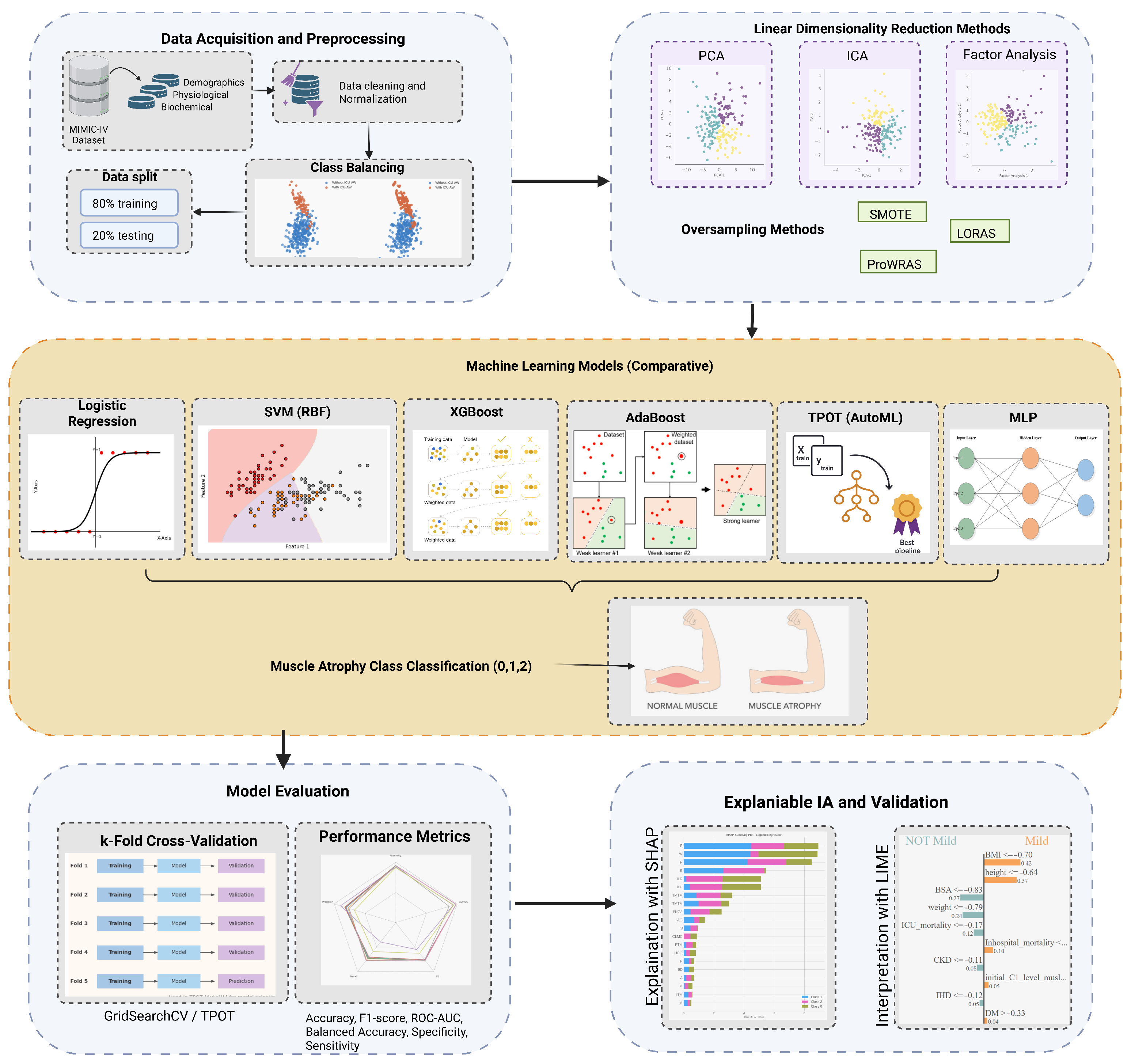
Figure 1.
Abstract Methodology.
Figure 1.
Abstract Methodology.
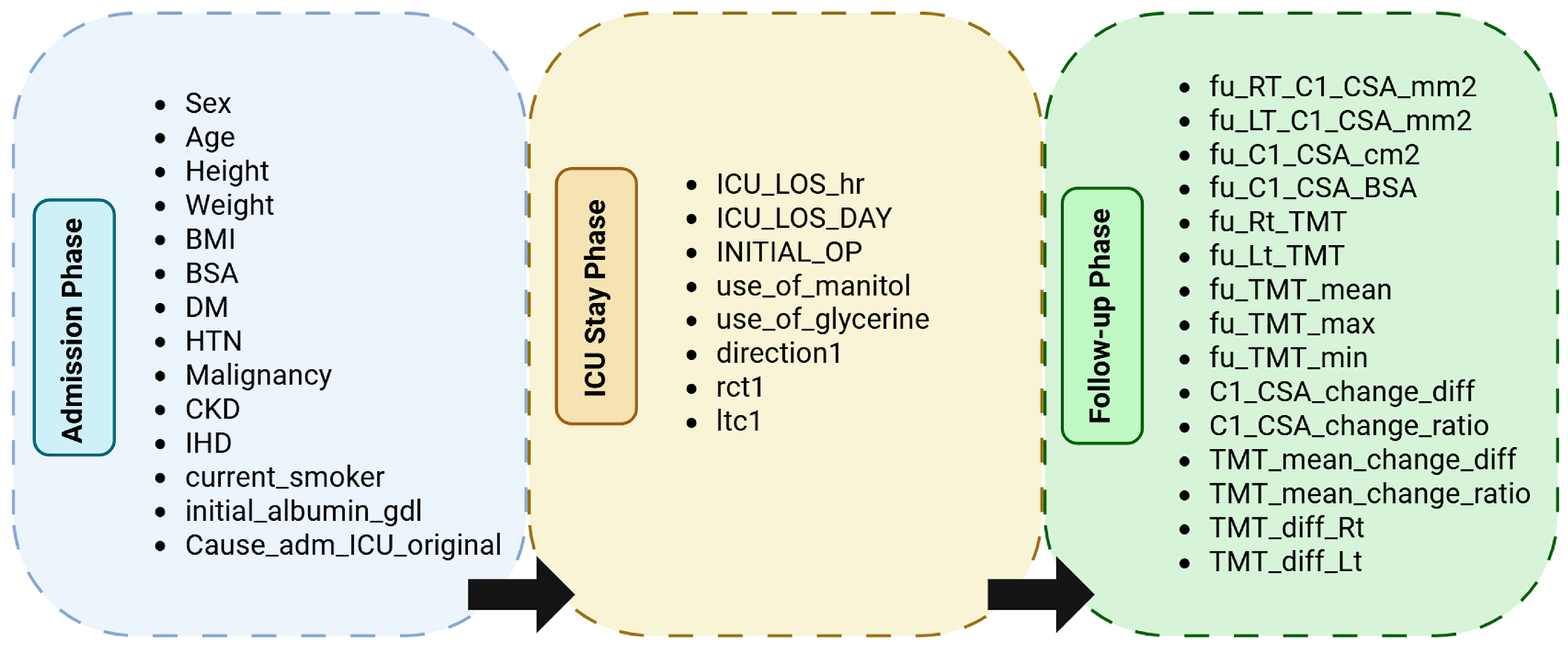
Figure 2.
Hierarchical grouping of variables by temporal phase in the dataset. Each phase corresponds to the clinical context of data acquisition: Admission (demographic and baseline measures), ICU Stay (therapeutic and monitoring data), and Follow-up (post-ICU morphometric and outcome variables).
Figure 2.
Hierarchical grouping of variables by temporal phase in the dataset. Each phase corresponds to the clinical context of data acquisition: Admission (demographic and baseline measures), ICU Stay (therapeutic and monitoring data), and Follow-up (post-ICU morphometric and outcome variables).
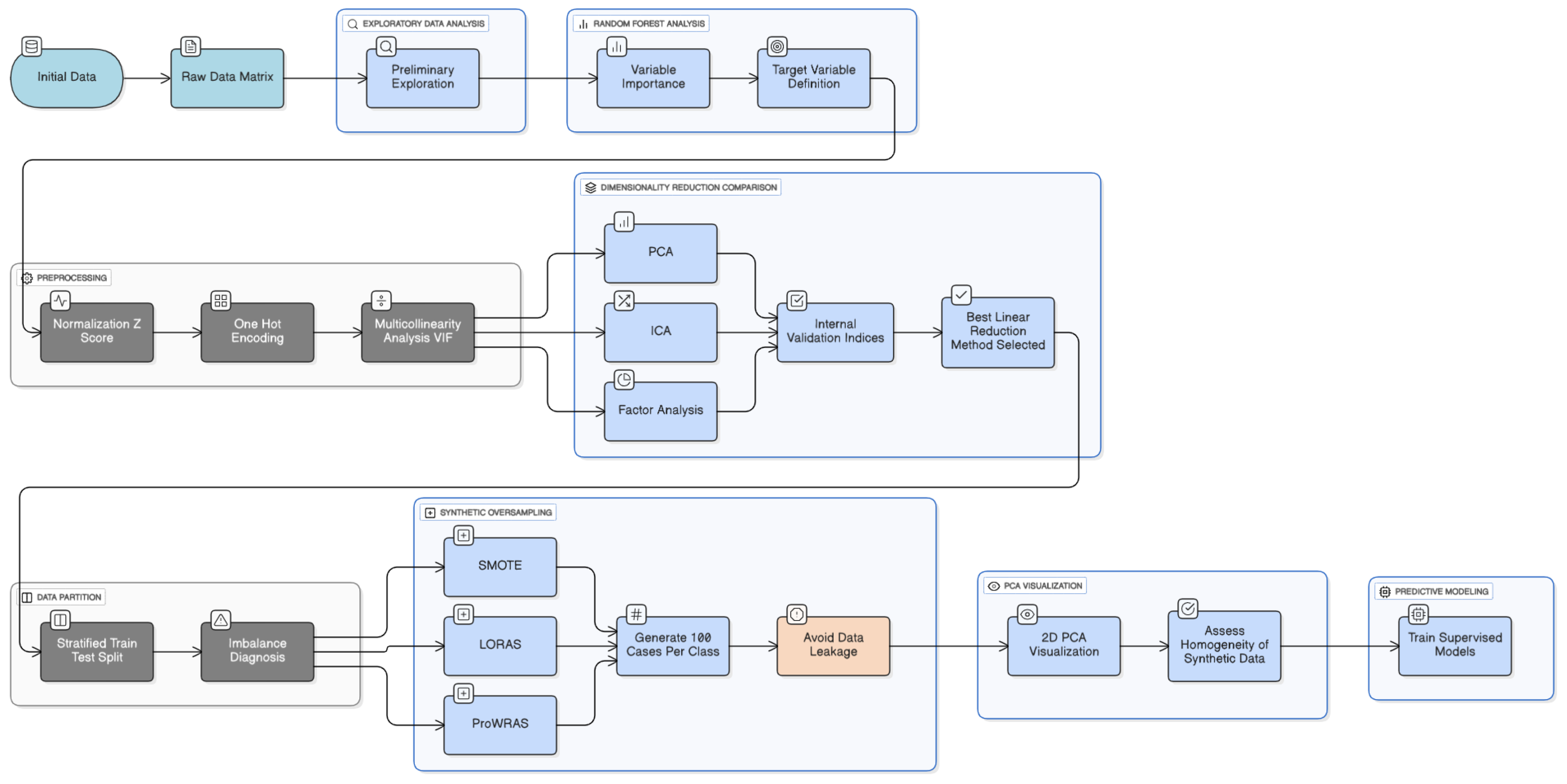
Figure 3.
Methodology of preprocessing data.
Figure 3.
Methodology of preprocessing data.
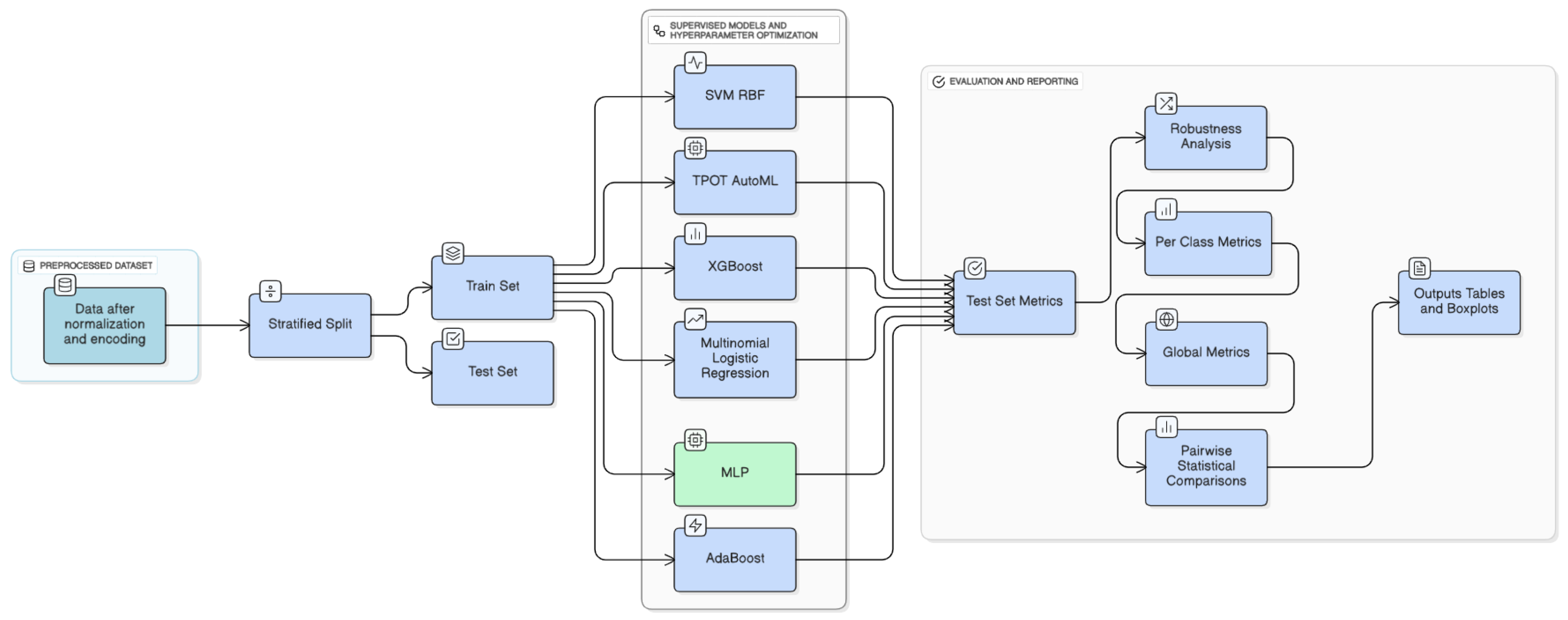
Figure 4.
Methodology of machine learning models implemented.
Figure 4.
Methodology of machine learning models implemented.
Figure 5.
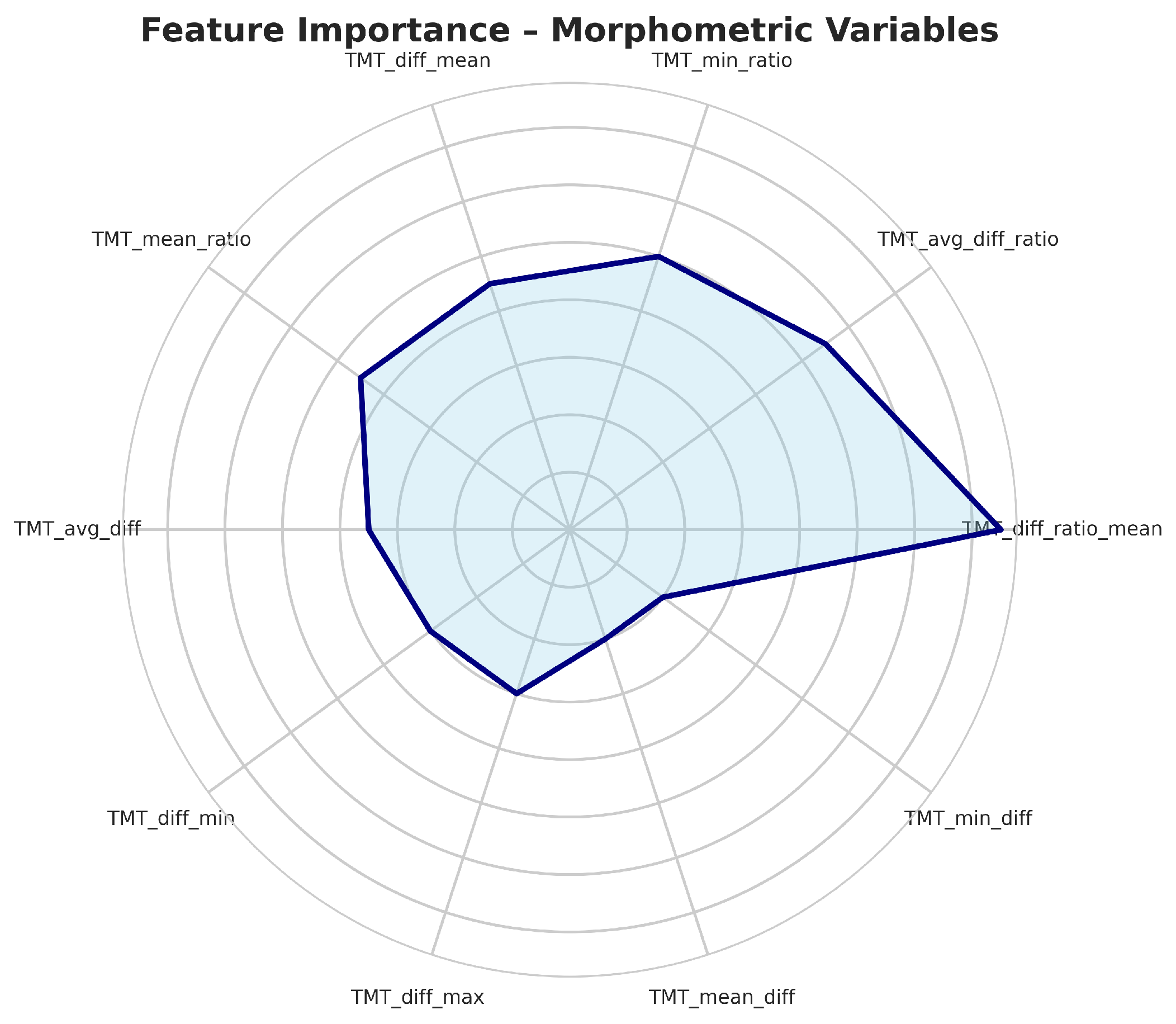
Top most important variables in data set.
Figure 5.
Top most important variables in data set.
Figure 6.
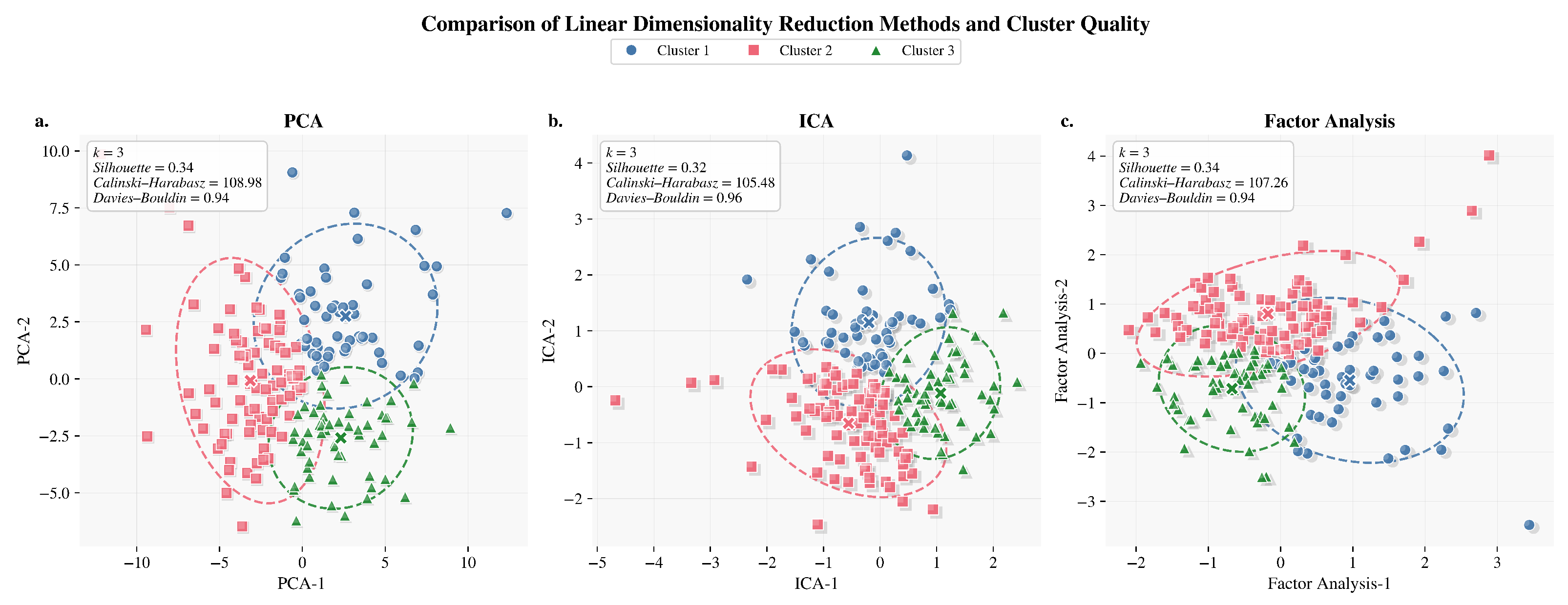
Linear dimensionality reduction comparison methods. (a) PCA: projection of three clusters in two principal components. (b) ICA: cluster separation in independent component space. (c) Factor Analysis: representation of linear separability across factors.
Figure 6.
Linear dimensionality reduction comparison methods. (a) PCA: projection of three clusters in two principal components. (b) ICA: cluster separation in independent component space. (c) Factor Analysis: representation of linear separability across factors.
Figure 7.
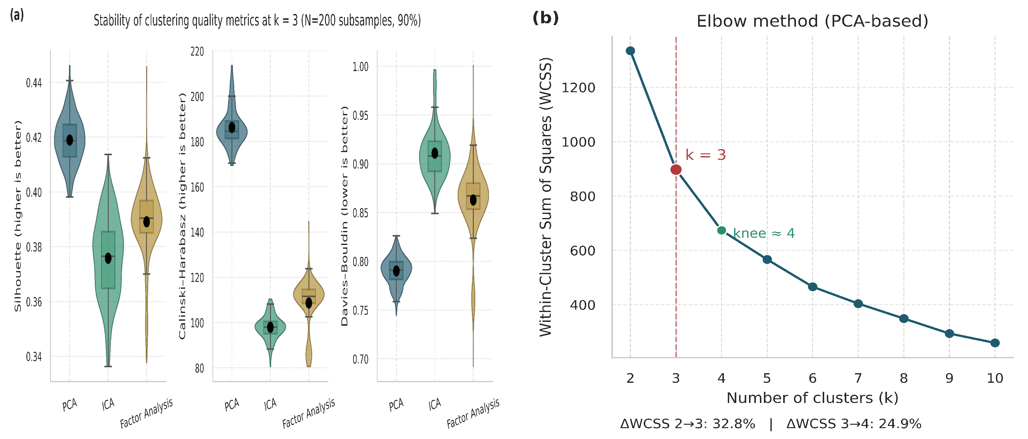
Validation and justification of the selected number of clusters (). (a) Violin and boxplot distributions representing the stability and dispersion of clustering metrics across multiple iterations. (b) Elbow plot based on PCA embeddings.
Figure 7.
Validation and justification of the selected number of clusters (). (a) Violin and boxplot distributions representing the stability and dispersion of clustering metrics across multiple iterations. (b) Elbow plot based on PCA embeddings.
Figure 8.
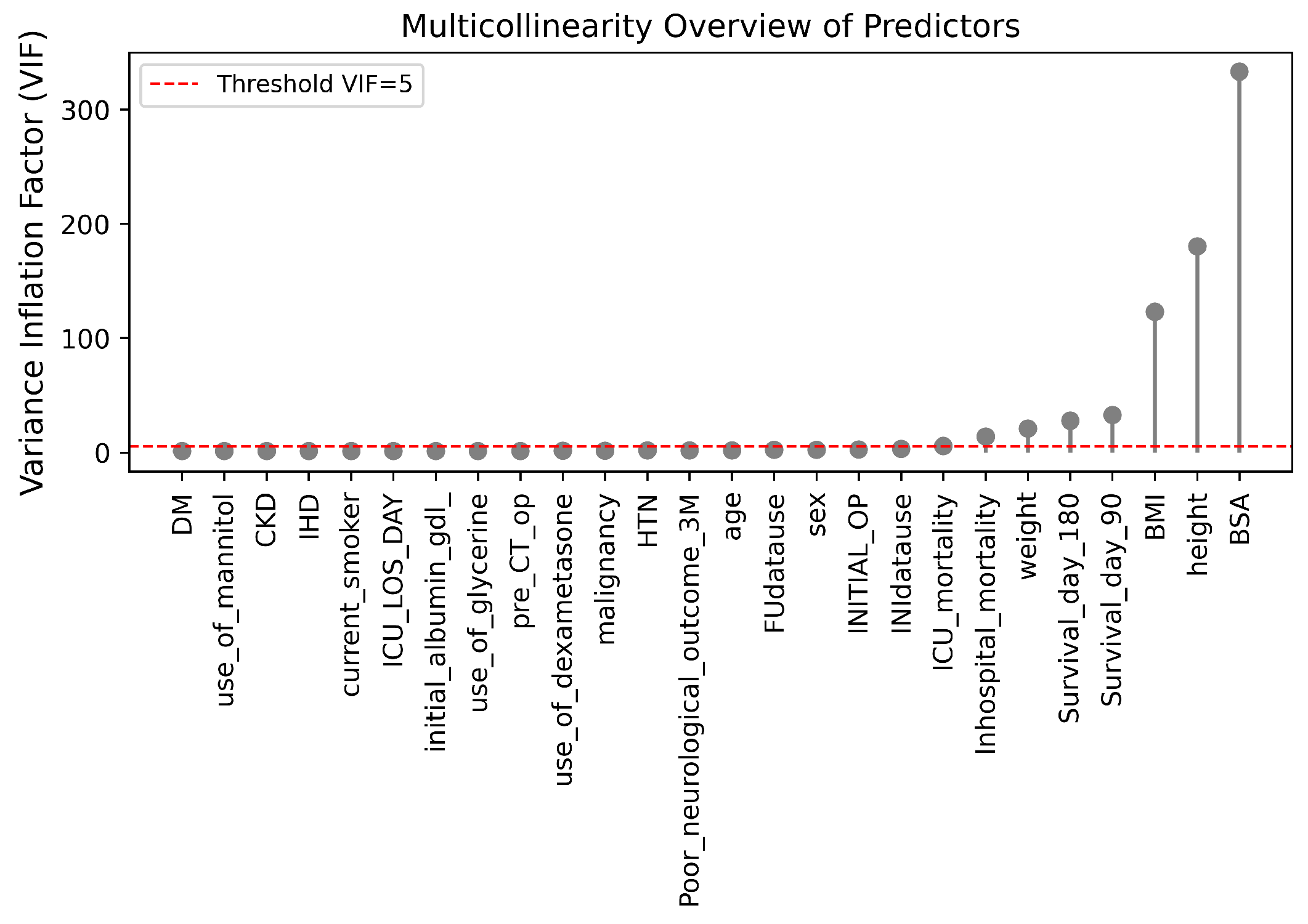
VIF of multicollinearity among predictors.
Figure 8.
VIF of multicollinearity among predictors.
Figure 9.
Oversampling methods comparison in PCA space. (a) Real vs SMOTE samples visualized in PCA space, showing synthetic data distribution around real instances. (b) Real vs LORAS samples demonstrating better boundary diversity and reduced overlap. (c) Real vs ProWRAS samples depicting improved class representation and structural preservation.
Figure 10.
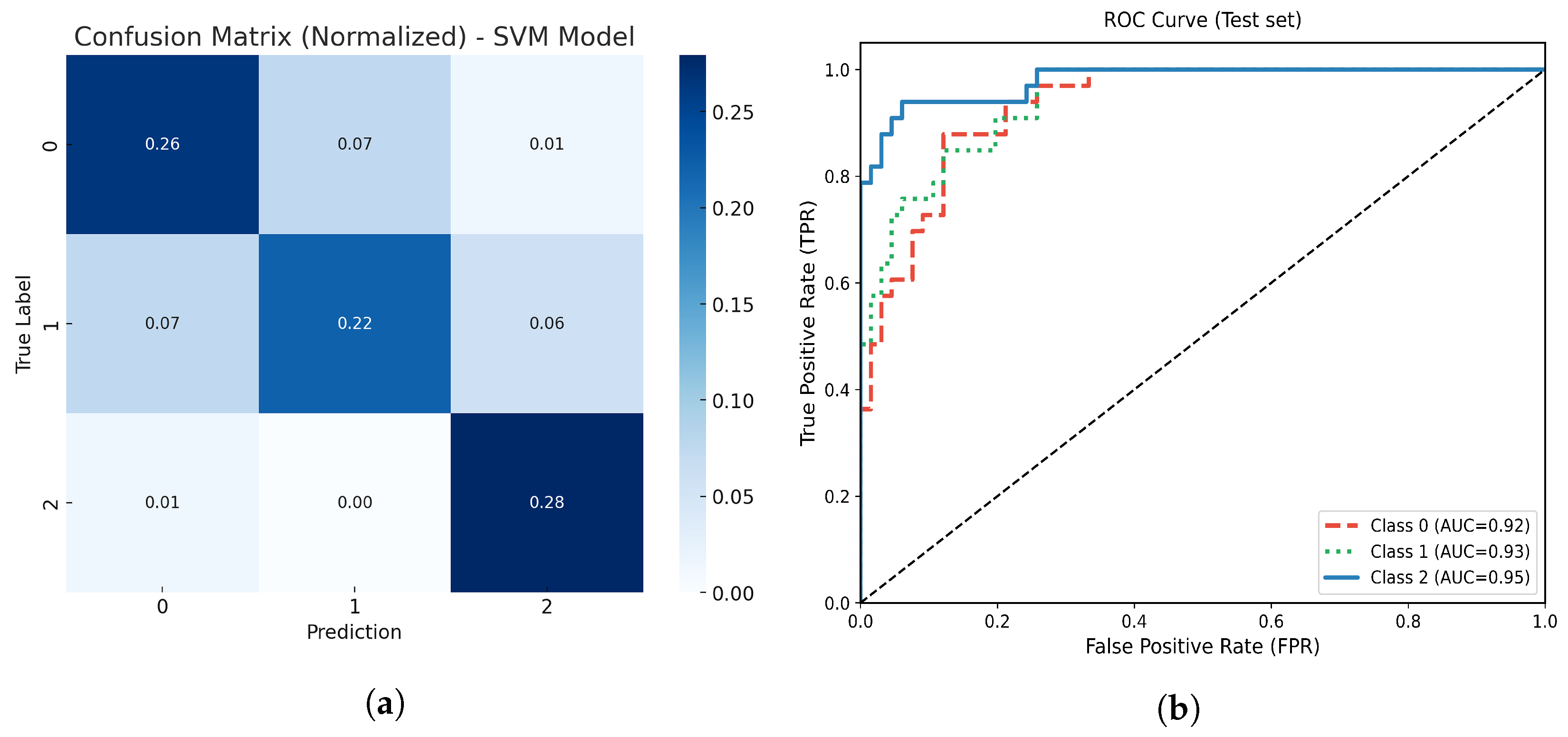
(a) Normalized confusion matrix for the optimized SVM model. (b) Multiclass ROC-AUC curves for each atrophy class.
Figure 10.
(a) Normalized confusion matrix for the optimized SVM model. (b) Multiclass ROC-AUC curves for each atrophy class.
Figure 11.
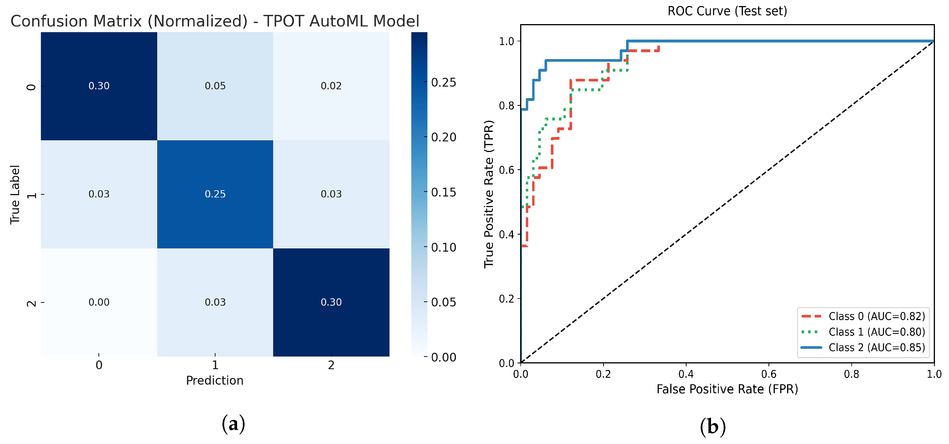
(a) Normalized confusion matrix for the optimized TPOT AutoML model. (b) Multiclass ROC-AUC curves for each atrophy class.
Figure 11.
(a) Normalized confusion matrix for the optimized TPOT AutoML model. (b) Multiclass ROC-AUC curves for each atrophy class.
Figure 12.
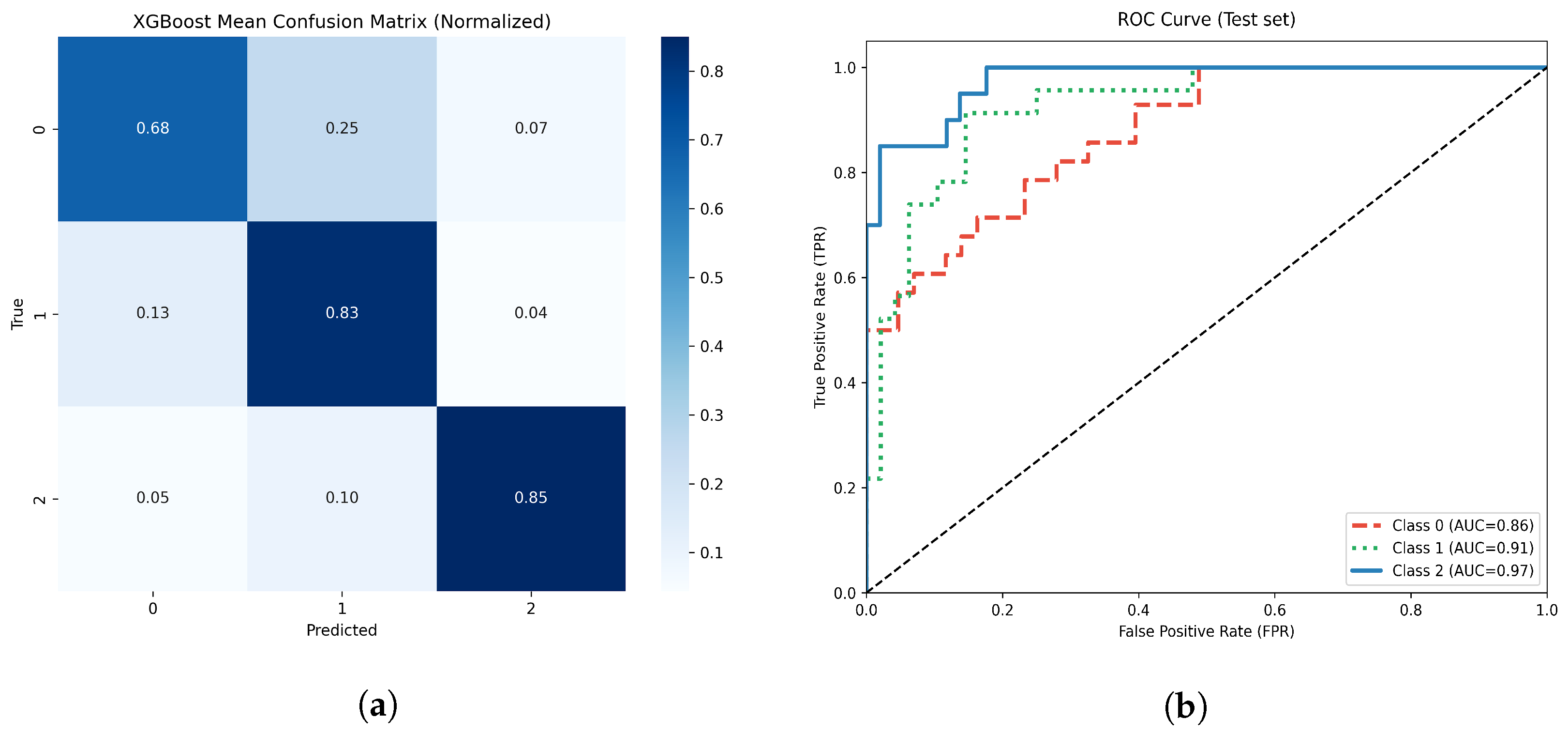
(a) Normalized confusion matrix for the optimized XGBoost model. (b) Multiclass ROC-AUC curves for each atrophy class.
Figure 12.
(a) Normalized confusion matrix for the optimized XGBoost model. (b) Multiclass ROC-AUC curves for each atrophy class.
Figure 13.
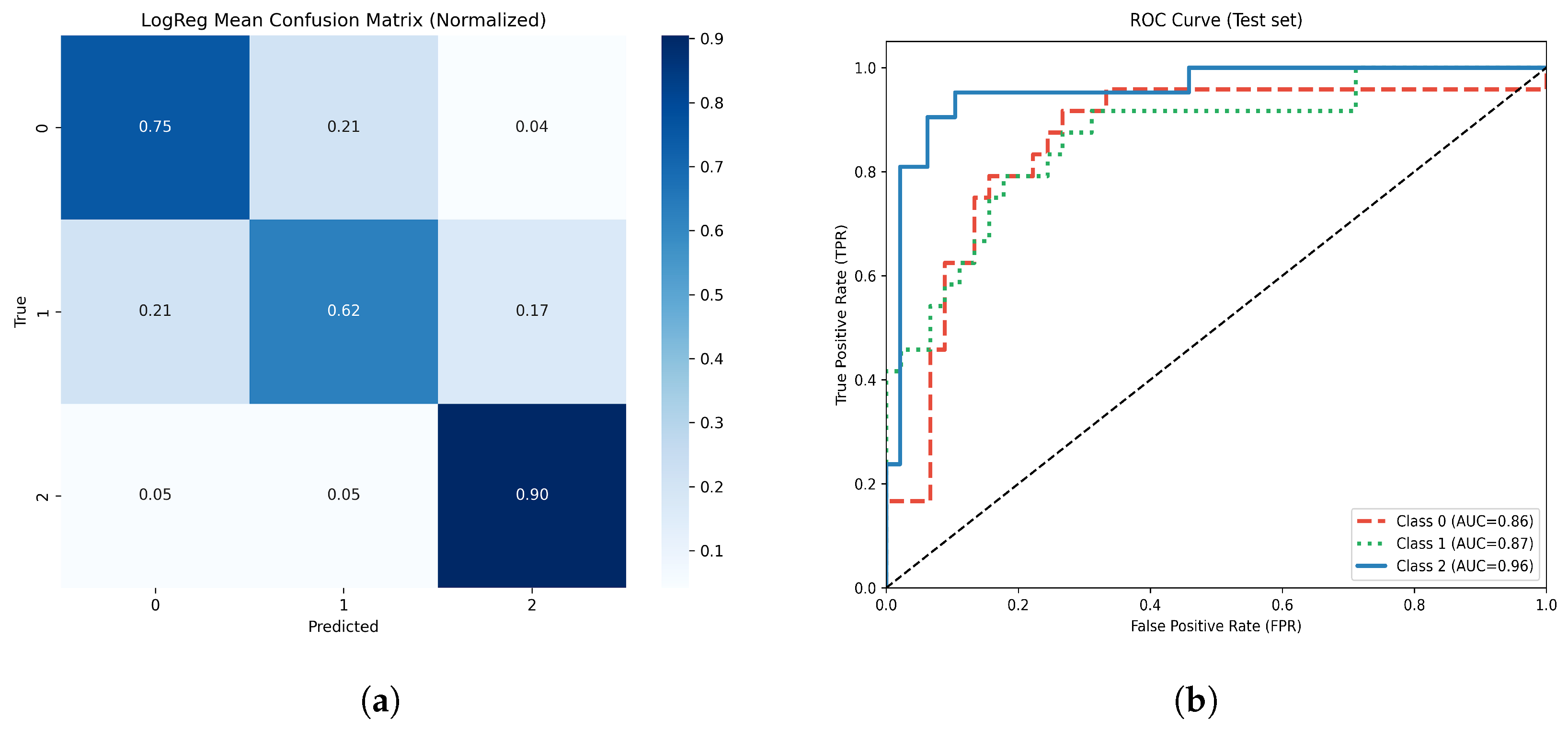
(a) Normalized confusion matrix for the optimized Logistic Regression model. (b) Multiclass ROC-AUC curves for each atrophy class.
Figure 13.
(a) Normalized confusion matrix for the optimized Logistic Regression model. (b) Multiclass ROC-AUC curves for each atrophy class.
Figure 14.
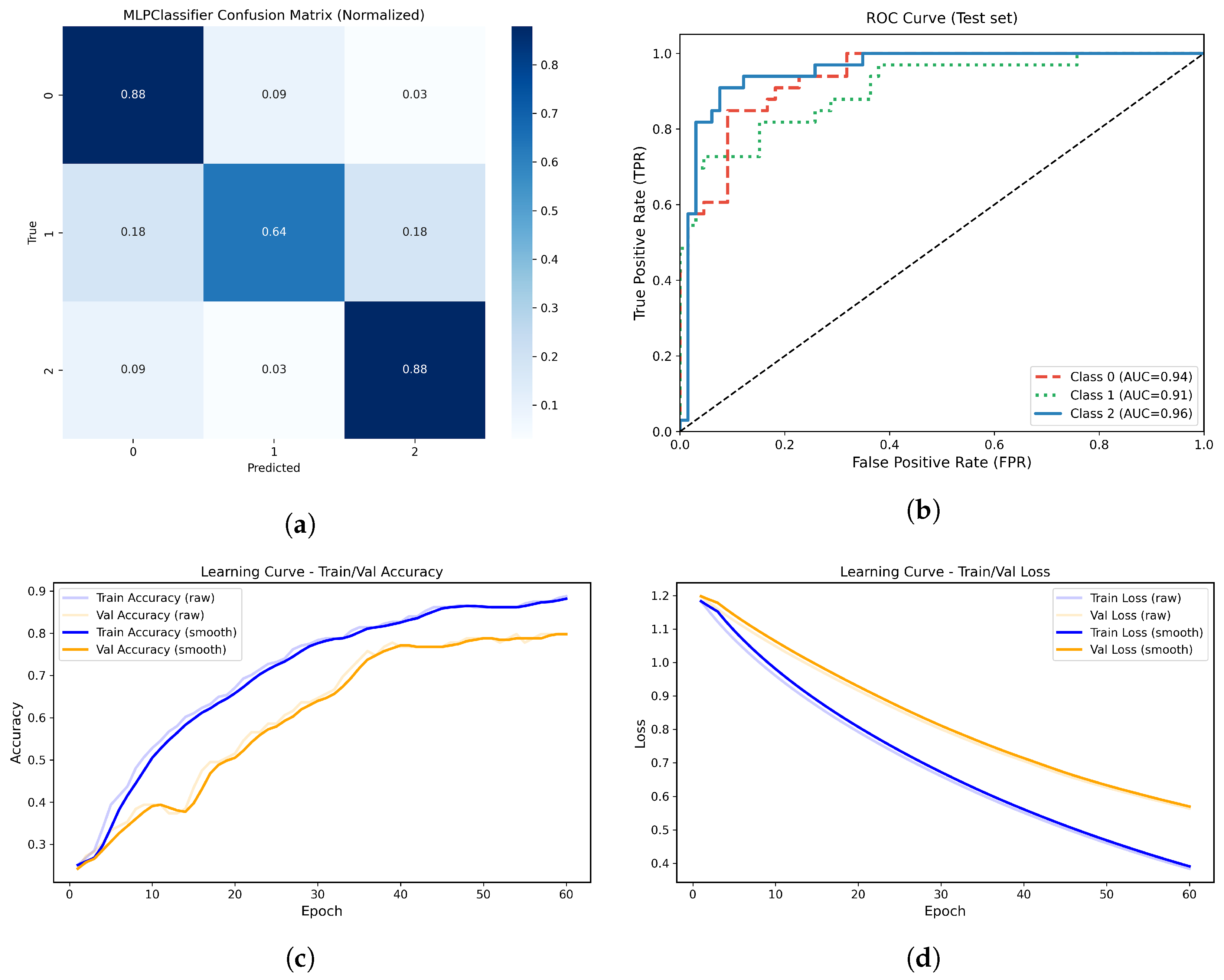
(a) Normalized confusion matrix for the MLPClassifier model. (b) Multiclass ROC-AUC curves for each atrophy class. (c) Learning curve showing training and validation accuracy across epochs. (d) Learning curve showing the progressive decrease in training and validation loss across epochs.
Figure 14.
(a) Normalized confusion matrix for the MLPClassifier model. (b) Multiclass ROC-AUC curves for each atrophy class. (c) Learning curve showing training and validation accuracy across epochs. (d) Learning curve showing the progressive decrease in training and validation loss across epochs.
Figure 15.
(a) Normalized confusion matrix for the optimized AdaBoost model. (b) Multiclass ROC-AUC curves for each atrophy class.
Figure 15.
(a) Normalized confusion matrix for the optimized AdaBoost model. (b) Multiclass ROC-AUC curves for each atrophy class.
Figure 16.
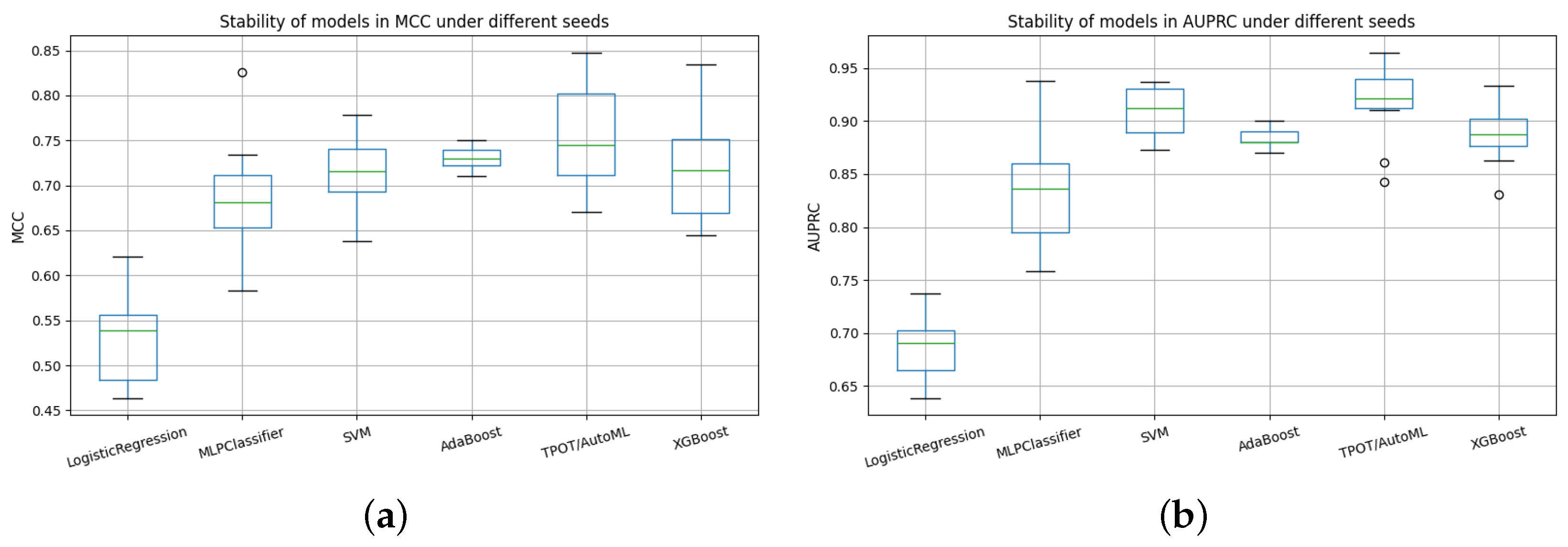
Comparative stability of models across random seeds using AUPRC and MCC metrics. (a) Stability of models in AUPRC under different seeds. (b) Stability of models in MCC under different seeds.
Figure 16.
Comparative stability of models across random seeds using AUPRC and MCC metrics. (a) Stability of models in AUPRC under different seeds. (b) Stability of models in MCC under different seeds.
Figure 17.
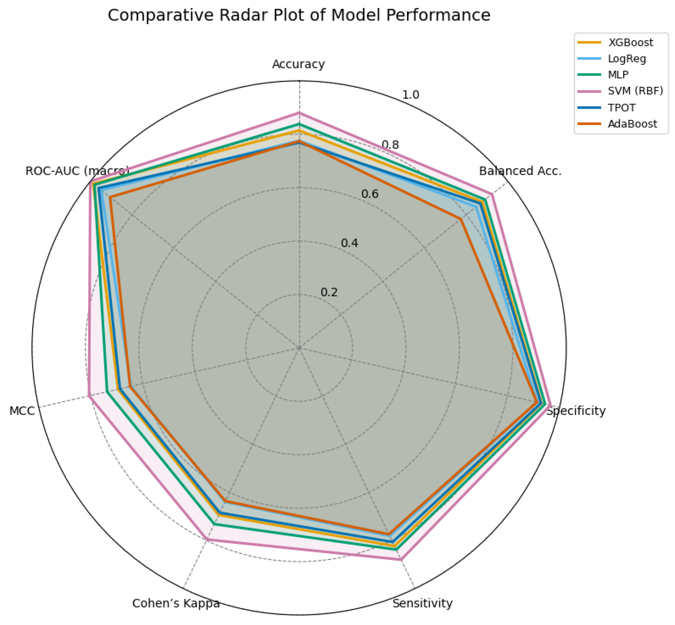
Radar comparison of extended evaluation metrics across all models. A larger enclosed area indicates a more balanced and stable performance. The SVM (RBF) model demonstrates superior overall consistency, followed by the MLP and XGBoost models.
Figure 17.
Radar comparison of extended evaluation metrics across all models. A larger enclosed area indicates a more balanced and stable performance. The SVM (RBF) model demonstrates superior overall consistency, followed by the MLP and XGBoost models.
Figure 18.
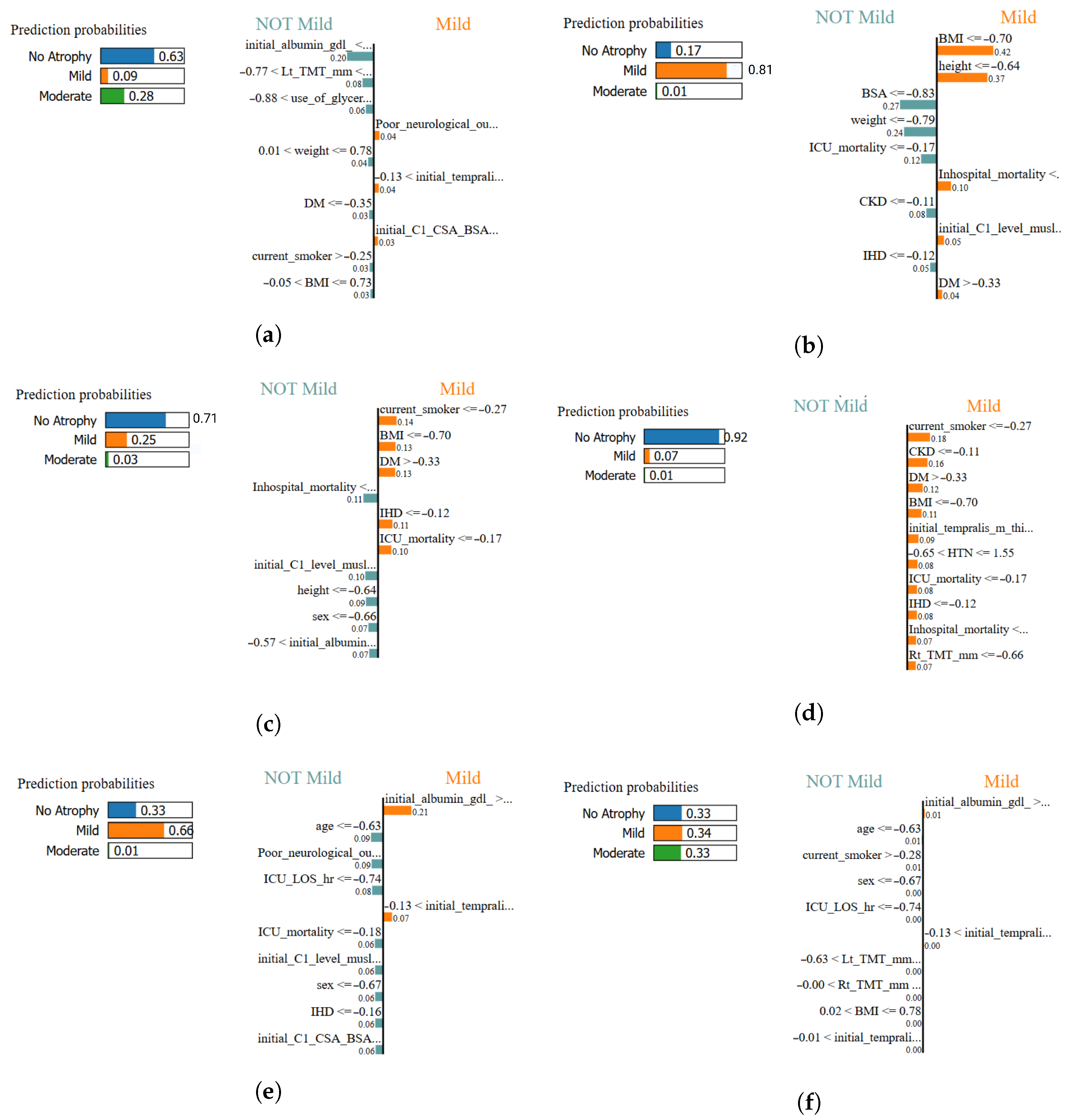
Local interpretability comparison using LIME across all classifiers. Each panel illustrates the most influential features contributing positively or negatively to the classification of muscle atrophy class for a representative test sample: (a) XGBoost–LIME explanation, (b) Logistic Regression–LIME explanation, (c) MLPClassifier–LIME explanation, (d) SVM (RBF)–LIME explanation, (e) TPOT AutoML–LIME explanation, and (f) AdaBoost–LIME explanation. In this study, the most influential features highlighted by LIME are primarily associated with anthropometric measures and clinical variables.
Table 1.
Summary of selected research articles on the application of machine learning in intensive care and neuromuscular rehabilitation.
Table 1.
Summary of selected research articles on the application of machine learning in intensive care and neuromuscular rehabilitation.
| Ref | Description | Type of Study | Use ML/AI | Data Modality |
|---|
| [9] | Combined ultrasound and inflammatory biomarkers for early ICU-AW detection. | Experimental | Yes | Bimodal (Ultrasound + Biomarkers) |
| [12] | Used supervised ML to predict ICU-AW from clinical and biochemical data. | Retrospective cohort | Yes | Unimodal (Clinical) |
| [22] | Compared multiple circulating biomarkers for ICU-AW diagnosis. | Systematic review | Partial | Unimodal (Biochemical) |
| [23] | Applied CNNs on electrophysiological data to assess neuromuscular activity. | Experimental | Yes | Unimodal (Electrophysiology) |
| [2] | Evaluated clinical predictors of ICU-AW without ML integration. | Observational | No | Clinical data |
| [24] | Reviewed AI applications in neuromuscular disorder diagnosis and therapy. | Literature review | Yes | Neuromuscular datasets |
| [25] | Described AI and robotics in physiotherapy and neurorehabilitation. | Review | Yes | Physiotherapy data |
| This study | Integrates multimodal clinical, biochemical, and morphometric data for ICU-AW severity classification. | Cross-sectional classification | Yes | Multimodal (Clinical + Biochemical + Morphometric) |
Table 2.
Main demographic and clinical characteristics of the cohort (n = 198).
Table 2.
Main demographic and clinical characteristics of the cohort (n = 198).
| Variable | Mean ± SD/n (%) |
|---|
| Age (years) | 58.3 ± 14.6 |
| Male sex | 103 (52%) |
| ICU length of stay (days) | 17.9 ± 6.4 |
| Mechanical ventilation | 142 (71.7%) |
| Hypertension | 95 (48%) |
| Diabetes mellitus | 64 (32%) |
| Serum albumin (g/dL) | 3.1 ± 0.6 |
| Body surface area (m2) | 1.78 ± 0.23 |
Table 3.
Continuous variables included in the analysis (n = 198).
Table 3.
Continuous variables included in the analysis (n = 198).
| Variable | Description | Unit |
|---|
| age | Age at ICU admission | years |
| height | Patient height | cm |
| weight | Patient weight | kg |
| BMI | Body Mass Index | kg/m2 |
| BSA | Body Surface Area | m2 |
| initial_albumin_gdl_ | Initial serum albumin | g/dL |
| initial_C1_level_muslce_CSA | Initial C1 muscle cross-sectional area | mm2 |
| initial_C1_CSA_BSA | Initial C1 CSA normalized by BSA | mm2/m2 |
| Rt_TMT_mm | Right temporalis muscle thickness | mm |
| Lt_TMT_mm | Left temporalis muscle thickness | mm |
| initial_tempralis_m_thickness_mean | Initial temporalis mean thickness | mm |
| initial_tempralis_m_thickness_max | Initial temporalis maximum thickness | mm |
| initial_tempralis_m_thickness_min | Initial temporalis minimum thickness | mm |
| fu_Rt_TMT | Follow-up right TMT | mm |
| fu_Lt_TMT | Follow-up left TMT | mm |
| fu_TMT_mean | Follow-up mean TMT | mm |
| fu_TMT_max | Follow-up maximum TMT | mm |
| fu_TMT_min | Follow-up minimum TMT | mm |
| fu_C1_CSA_BSA | Follow-up C1 CSA normalized by BSA | cm2/m2 |
| C1_CSA_change_diff | Absolute change in C1 CSA | mm2 |
| C1_CSA_BSA_change_ratio | Relative change in C1 CSA/BSA | ratio |
| TMT_max_change_diff | Absolute change in TMT (max) | mm |
| TMT_mean_change_diff | Mean TMT change difference | mm |
| TMT_min_change_diff | Minimum TMT change difference | mm |
| TMT_diff_Rt | Right TMT difference | mm |
| TMT_diff_Lt | Left TMT difference | mm |
| TMT_diff_mean | Mean TMT difference | mm |
| TMT_diff_ratio_mean | Mean TMT ratio difference | ratio |
| TMT_diff_ratio_max | Maximum TMT ratio difference | ratio |
| TMT_diff_ratio_min | Minimum TMT ratio difference | ratio |
| TMT_mean_change_ratio | Average change ratio in TMT | ratio |
| TMT_min_change_ratio | Minimum change ratio in TMT | ratio |
| TMT_average_change_diff | Average absolute TMT change | mm |
| TMT_average_change_diff_ratio | Average relative TMT change ratio | ratio |
| ICU_LOS_DAY | ICU length of stay | days |
| Survival_day_90 | Survival time at 90 days | days |
| Survival_day_180 | Survival time at 180 days | days |
Table 4.
Categorical and binary variables included in the analysis (n = 198).
Table 4.
Categorical and binary variables included in the analysis (n = 198).
| Variable | Description | Unit |
|---|
| sex | Biological sex (0 = Female, 1 = Male) | - |
| DM | Diabetes mellitus (0 = No, 1 = Yes) | - |
| HTN | Hypertension (0 = No, 1 = Yes) | - |
| malignancy | Any malignancy (0 = No, 1 = Yes) | - |
| CKD | Chronic kidney disease (0 = No, 1 = Yes) | - |
| IHD | Ischemic heart disease (0 = No, 1 = Yes) | - |
| current_smoker | Current smoker (0 = No, 1 = Yes) | - |
| INITIAL_OP | Initial operative management (0/1) | - |
| pre_CT_op | Pre-CT operation (0/1) | - |
| ICU_mortality | ICU mortality (0/1) | - |
| Inhospital_mortality | In-hospital mortality (0/1) | - |
| GOS_3M | Glasgow Outcome Scale at 3 months (ordinal 1–5) | ordinal |
| Poor_neurological_outcome_3M | Poor neurological outcome (GOS ≤ 3) | - |
| use_of_mannitol | Use of mannitol (0/1) | - |
| use_of_glycerine | Use of glycerine (0/1) | - |
| use_of_dexametasone | Use of dexamethasone (0/1) | - |
Table 5.
Comparative landscape of public ICU datasets for ML on neuromuscular outcomes.
Table 5.
Comparative landscape of public ICU datasets for ML on neuromuscular outcomes.
| Dataset | Size | EHR/Labs | High-Res Vitals | Imaging | Neurom. Data | Functional Outcomes | Ref. |
|---|
| Harvard DVN (this study) | n = 198, Neuro-ICU | Yes | – | Yes (US-based) | Yes (TMT/CSA, MRC) | Yes (3-months) | [26] |
| MIMIC-III | ∼60k ICU stays | Yes | Yes | – | – | – | [28] |
| eICU-CRD | Multi-center US | Yes | Yes | – | – | – | [29] |
| HiRID | Single-center, high-res | Yes | Yes (1-min) | – | – | – | [30] |
| UMCdb | Multi-center EU | Yes | Yes | – | – | – | [31] |
Table 6.
Configuration and optimization summary of supervised machine learning models for muscle atrophy classification.
Table 6.
Configuration and optimization summary of supervised machine learning models for muscle atrophy classification.
| Model (Library) | Configuration and Hyperparameters | Optimization Strategy |
|---|
| SVM (scikit-learn) | RBF kernel (, ); suitable for moderate-sized, high-dimensional data with non-linear relationships. | GridSearchCV (5-fold cross-validation). |
| TPOT AutoML (tpot) | Genetic programming-based AutoML; population = 100, generations = 15; automatic pipeline exploration and early stopping. | Evolutionary optimization with internal cross-validation. |
| XGBoost (xgboost) | Gradient-boosted decision trees; tuned parameters: max_depth, learning_rate, n_estimators, subsample, colsample_bytree, reg_alpha, reg_lambda. | RandomizedSearchCV (15 iterations, 4-fold CV). |
| Multinomial Logistic Regression (scikit-learn) | Baseline linear model with L2 regularization; solvers: lbfgs, saga, newton-cg; maximum 500 iterations. | GridSearchCV (4-fold CV) to optimize C and ensure convergence. |
| MLP (scikit-learn) | Single hidden layer (60 neurons), ReLU activation, Adam optimizer, learning rate = 0.001, L2 regularization (); trained for 60 epochs. | Learning curves monitored for training and validation accuracy/loss. |
| AdaBoost (scikit-learn) | Base estimator: DecisionTreeClassifier (max_depth = 2); 120 estimators, learning rate = 0.8, random state = 42. | Direct evaluation with consistent preprocessing across models. |
|
Evaluation Metrics (common to all models) | Global: Accuracy, Macro F1, ROC–AUC, AUPRC, Log Loss, MCC, Cohen’s Kappa.
Per–class: Recall, Precision, Specificity, Balanced Accuracy, F2–Score.
Robustness: 10 random seeds with seed-dependent AUPRC and MCC variability.
Interpretability: SHAP (global) and LIME (local) analyses for explainability. | Applied consistently across all algorithms for performance benchmarking and validation stability. |
Table 7.
Comparative clustering quality metrics across linear dimensionality reduction methods.
Table 7.
Comparative clustering quality metrics across linear dimensionality reduction methods.
| Method | Silhouette | Calinski–Harabasz | Davies–Bouldin |
|---|
| PCA | 0.34 | 108.98 | 0.94 |
| ICA | 0.32 | 105.48 | 0.96 |
| Factor Analysis | 0.34 | 107.26 | 0.94 |
Table 8.
Data-driven classification of muscle atrophy levels based on morphometric parameters (TMT and CSA).
Table 8.
Data-driven classification of muscle atrophy levels based on morphometric parameters (TMT and CSA).
| Atrophy Level | Definition Criteria |
|---|
| No atrophy | Patients with preserved temporalis muscle thickness (TMT) and C1 cross-sectional area (CSA) within ±1 standard deviation of the cohort mean. |
| Mild atrophy | Individuals showing moderate reductions in either TMT or CSA between 1–2 standard deviations below the cohort mean. |
| Moderate atrophy | Patients with severe reductions (>2 standard deviations below the mean) in both TMT and CSA, indicating significant muscle wasting. |
Table 9.
Comparative distributional fidelity metrics for oversampling algorithms in PCA-reduced morphometric space. Lower values indicate higher similarity between real and synthetic data distributions.
Table 9.
Comparative distributional fidelity metrics for oversampling algorithms in PCA-reduced morphometric space. Lower values indicate higher similarity between real and synthetic data distributions.
| Method | KLPC1 | WDPC1 | KLPC2 | WDPC2 |
|---|
| SMOTE | 0.0302 | 0.5712 | 0.0227 | 0.0849 |
| LORAS | 0.0667 | 0.6900 | 0.0412 | 0.2007 |
| ProWRAS | 0.0631 | 0.7244 | 0.0551 | 0.2382 |
Table 10.
Comparative performance of six supervised ML models for muscle atrophy classification.
Table 10.
Comparative performance of six supervised ML models for muscle atrophy classification.
| Condition | Metric | SVM (RBF) | TPOT/AutoML | XGBoost | Logistic Reg. | MLPClassifier | AdaBoost |
|---|
| Precision | 0.920 | 0.820 | 0.826 | 0.850 | 0.763 | 0.650 |
| No Atrophy (0) | Recall | 0.910 | 0.790 | 0.679 | 0.762 | 0.879 | 0.788 |
| | F1-score | 0.915 | 0.805 | 0.745 | 0.750 | 0.817 | 0.716 |
| Precision | 0.930 | 0.800 | 0.701 | 0.714 | 0.840 | 0.690 |
| Mild (1) | Recall | 0.920 | 0.780 | 0.826 | 0.625 | 0.736 | 0.545 |
| | F1-score | 0.915 | 0.790 | 0.745 | 0.667 | 0.724 | 0.679 |
| Precision | 0.950 | 0.850 | 0.920 | 0.792 | 0.806 | 0.744 |
| Moderate (2) | Recall | 0.930 | 0.830 | 0.850 | 0.905 | 0.879 | 0.879 |
| | F1-score | 0.940 | 0.840 | 0.894 | 0.844 | 0.841 | 0.806 |
| Mean F1 | 0.928 | 0.810 | 0.795 | 0.754 | 0.794 | 0.732 |
| Overall | Weighted F1 | 0.931 | 0.820 | 0.795 | 0.759 | 0.801 | 0.732 |
| | Accuracy | 0.930 | 0.810 | 0.800 | 0.794 | 0.828 | 0.737 |
Table 11.
AUPRC results by seed for the different classification models.
Table 11.
AUPRC results by seed for the different classification models.
| Seed | Logistic Regression | MLPClassifier | SVM | TPOT/AutoML | XGBoost | AdaBoost |
|---|
| 0 | 0.6821 | 0.8031 | 0.8539 | 0.9070 | 0.9116 | 0.8217 |
| 1 | 0.7458 | 0.8462 | 0.8816 | 0.8941 | 0.8396 | 0.7635 |
| 2 | 0.8187 | 0.9569 | 0.9748 | 0.9809 | 0.8990 | 0.8641 |
| 3 | 0.7112 | 0.8146 | 0.9318 | 0.9105 | 0.8939 | 0.7916 |
| 4 | 0.6929 | 0.8261 | 0.8646 | 0.8876 | 0.8804 | 0.8196 |
| 5 | 0.6828 | 0.8329 | 0.8487 | 0.8959 | 0.8571 | 0.7447 |
| 6 | 0.7251 | 0.8130 | 0.8853 | 0.8952 | 0.8883 | 0.9101 |
| 7 | 0.7690 | 0.8719 | 0.9049 | 0.9118 | 0.8565 | 0.8079 |
| 8 | 0.7475 | 0.8798 | 0.9158 | 0.9165 | 0.9127 | 0.8262 |
| 9 | 0.6768 | 0.8216 | 0.9071 | 0.9384 | 0.8918 | 0.8196 |
Table 12.
MCC results by seed for the different classification models.
Table 12.
MCC results by seed for the different classification models.
| Seed | Logistic Regression | MLPClassifier | SVM | TPOT/AutoML | XGBoost | AdaBoost |
|---|
| 0 | 0.470 | 0.595 | 0.683 | 0.832 | 0.743 | 0.6674 |
| 1 | 0.549 | 0.639 | 0.713 | 0.681 | 0.782 | 0.5477 |
| 2 | 0.625 | 0.865 | 0.835 | 0.879 | 0.911 | 0.7446 |
| 3 | 0.427 | 0.752 | 0.688 | 0.745 | 0.623 | 0.6095 |
| 4 | 0.471 | 0.636 | 0.698 | 0.668 | 0.622 | 0.6086 |
| 5 | 0.364 | 0.668 | 0.648 | 0.780 | 0.668 | 0.5191 |
| 6 | 0.583 | 0.805 | 0.758 | 0.789 | 0.716 | 0.7605 |
| 7 | 0.534 | 0.731 | 0.776 | 0.655 | 0.654 | 0.6522 |
| 8 | 0.501 | 0.743 | 0.691 | 0.758 | 0.728 | 0.6456 |
| 9 | 0.471 | 0.643 | 0.732 | 0.774 | 0.743 | 0.6225 |
Table 13.
Per-class metrics for the different models, including AdaBoost.
Table 13.
Per-class metrics for the different models, including AdaBoost.
| Model | Class | Recall (TPR) | Specificity (TNR) | Precision | Balanced Acc | F2 Score | Support |
|---|
| XGBoost | 0 | 0.73 | 0.86 | 0.73 | 0.80 | 0.73 | 33 |
| | 1 | 0.61 | 0.91 | 0.77 | 0.76 | 0.63 | 33 |
| | 2 | 0.97 | 0.88 | 0.80 | 0.92 | 0.93 | 33 |
| Logistic Regression | 0 | 0.73 | 0.82 | 0.67 | 0.77 | 0.71 | 33 |
| | 1 | 0.48 | 0.83 | 0.59 | 0.66 | 0.50 | 33 |
| | 2 | 0.82 | 0.86 | 0.75 | 0.84 | 0.80 | 33 |
| MLPClassifier | 0 | 0.88 | 0.86 | 0.76 | 0.87 | 0.85 | 33 |
| | 1 | 0.64 | 0.94 | 0.84 | 0.79 | 0.67 | 33 |
| | 2 | 0.88 | 0.89 | 0.81 | 0.89 | 0.86 | 33 |
| SVM (RBF) | 0 | 0.91 | 0.83 | 0.73 | 0.87 | 0.87 | 33 |
| | 1 | 0.67 | 0.98 | 0.96 | 0.83 | 0.71 | 33 |
| | 2 | 0.94 | 0.94 | 0.89 | 0.94 | 0.93 | 33 |
| TPOT/AutoML | 0 | 0.70 | 0.86 | 0.72 | 0.78 | 0.70 | 33 |
| | 1 | 0.70 | 0.92 | 0.82 | 0.81 | 0.72 | 33 |
| | 2 | 0.94 | 0.88 | 0.79 | 0.91 | 0.91 | 33 |
| AdaBoost | 0 | 0.76 | 0.82 | 0.68 | 0.79 | 0.74 | 33 |
| | 1 | 0.70 | 0.89 | 0.77 | 0.80 | 0.71 | 33 |
| | 2 | 0.79 | 0.91 | 0.81 | 0.85 | 0.79 | 33 |
Table 14.
Pairwise statistical comparisons between models (p-values).
Table 14.
Pairwise statistical comparisons between models (p-values).
| Comparison | p-Value | Interpretation |
|---|
| Logistic Regression vs. MLP | 0.436 | Not significant |
| Logistic Regression vs. SVM | 0.002 | Significant (SVM better) |
| Logistic Regression vs. TPOT | <0.001 | Highly significant (TPOT better) |
| Logistic Regression vs. XGB | 0.006 | Significant (XGBoost better) |
| MLP vs. SVM | 0.276 | Not significant |
| MLP vs. TPOT | 0.002 | Significant (TPOT better) |
| MLP vs. XGB | 0.436 | Not significant |
| SVM vs. TPOT | 0.436 | Not significant |
| SVM vs. XGB | ≈0.999 | Not significant |
| TPOT vs. XGB | 0.276 | Not significant |
Table 15.
Performance metrics of the evaluated machine learning models, including AdaBoost.
Table 15.
Performance metrics of the evaluated machine learning models, including AdaBoost.
| (a) Core Performance Metrics |
|---|
|
Model
|
Accuracy
|
Balanced Acc.
|
Specificity
|
Sensitivity
|
|---|
| XGBoost | 0.80 | 0.835 | 0.886 | 0.784 |
| LogReg | 0.794 | 0.807 | 0.870 | 0.744 |
| MLP | 0.828 | 0.848 | 0.899 | 0.798 |
| SVM (RBF) | 0.93 | 0.879 | 0.919 | 0.838 |
| TPOT | 0.81 | 0.826 | 0.884 | 0.768 |
| AdaBoost | 0.737 | 0.737 | 0.869 | 0.737 |
| (b) Extended Evaluation Metrics |
| Model | Cohen’s | MCC | ROC-AUC (Macro) | ROC-AUC (Micro) |
| XGBoost | 0.661 | 0.662 | 0.939 | 0.939 |
| LogReg | 0.609 | 0.615 | 0.902 | 0.904 |
| MLP | 0.697 | 0.702 | 0.933 | 0.931 |
| SVM (RBF) | 0.758 | 0.768 | 0.952 | 0.951 |
| TPOT | 0.652 | 0.655 | 0.914 | 0.914 |
| AdaBoost | 0.606 | 0.618 | 0.862 | 0.856 |
Table 16.
Interpretation summary of the XAI methods applied in this study. SHAP provides global interpretability across the dataset, while LIME offers local interpretability for individual classifications, ensuring both analytical and clinical transparency.
Table 16.
Interpretation summary of the XAI methods applied in this study. SHAP provides global interpretability across the dataset, while LIME offers local interpretability for individual classifications, ensuring both analytical and clinical transparency.
| Method | Explanation Scope | Key Insights | Clinical Interpretation |
|---|
| SHAP | Global (dataset-level) | Determines the overall contribution and directionality of features across all classifications. | Identifies BMI, BSA, ICU stay duration as dominant classifiers of muscle atrophy. |
| LIME | Local (instance-level) | Provides individualized explanations showing how specific variables influenced a single classification. | Confirms that patient-level decisions follow physiologically coherent patterns, supporting clinical trustworthiness. |
Table 17.
Top consensus features for multiclass muscle atrophy classification based on integrated mean importance across all machine learning models.
Table 17.
Top consensus features for multiclass muscle atrophy classification based on integrated mean importance across all machine learning models.
| Feature | Variable Type | Integrated Mean Importance |
|---|
| BSA (Body Surface Area) | Anthropometric | 0.72 |
| Height | Anthropometric | 0.71 |
| Temporal Muscle Thickness (min) | Imaging | 0.69 |
| HTN (Hypertension) | Clinical | 0.54 |
| Poor Neuro Outcome (3M) | Outcome | 0.63 |
| Albumin | Biochemical | 0.49 |
| C1 Muscle CSA | Imaging | 0.42 |
| BMI (Body Mass Index) | Anthropometric | 0.52 |
| Survival days | Outcome | 0.36 |
| Weight | Anthropometric | 0.38 |
Table 18.
Comparative overview of machine learning studies addressing muscle atrophy in critical and neurocritical care, distinguishing predictive and classification approaches.
Table 18.
Comparative overview of machine learning studies addressing muscle atrophy in critical and neurocritical care, distinguishing predictive and classification approaches.
| Reference | Cohort/Setting | ML Model(s) | Primary Task | Performance (Acc/AUC) |
|---|
| I. Predictive Models (ICU-AW Onset/Risk Prediction) |
| [38] | NeuroICU (n = 120, TBI/stroke) | SVM, Random Forest | Predict ICU-AW onset using electrophysiology, TMT, BMI, albumin | AUC ≈ 0.92 (SVM) |
| [39] | Multicenter ICU (n = 210) | XGBoost, Logistic Regression | Predict ICU-AW risk from ultrasound, SOFA, hypertension | Acc. ≈ 0.85 (XGB) |
| [12] | ICU (sepsis subgroup, n = 184) | LR, RF, XGB (+LASSO) | Predict ICU-AW from cytokines, APACHE II, albumin | Acc. ≈ 0.88 |
| [43] | ICU (MV ≥ 7d, n = 97) | LASSO, RF, LR | Predict poor mobility outcome from SAPS 3 + Perme scale | Acc. ≈ 0.80 |
| [37] | ICU (prospective, n = 749) | XGBoost, RF, SVM, LR | Predict ICU-AW from multimodal clinical + lab + US data | Acc. = 0.978 (XGB) |
| II. Classification Models (Atrophy Severity/Neuromuscular Grading) |
| [9] | Septic ICU (n = 128) | Random Forest, Logistic Regression | Classify three-grade ICU-AW severity (MRC-based) | AUC = 0.83 (RF) |
| [42] | Sarcopenia (n = 40) | CNN U-Net | Classify binary (CT muscle area) | Acc. = 0.96 |
| [44] | Neuro-oncology (GBM) | CNN (Deep Learning) | Classify temporalis atrophy index (CSA segmentation) | AUC = 0.84 |
| [45] | MRI neuro dataset (n = 23,876) | DL pipeline (iTMT) | Automated grading of TMT (percentile-based) | AUC = 0.90 |
| [46] | Acute ischemic stroke (n = 264) | Deep CNN (MRI) | Dichotomous classification: severe vs. non-severe TMT loss | AUC = 0.85 |
| Present study | NeuroICU (n = 198) | SVM, XGB, MLP, AdaBoost, TPOT, Logistic | Three-class atrophy severity (no, mild, moderate) | Acc. = 0.93; AUC = 0.95 (SVM) |
