Abstract
We present a simple mathematical model that captures the evolutionary capabilities of a prebiotic compartment or protocell. In the model, the protocell contains an autocatalytic set whose chemical dynamics is coupled to the growth–division dynamics of the compartment. Bistability in the dynamics of the autocatalytic set results in a protocell that can exist with two distinct growth rates. Stochasticity in chemical reactions plays the role of mutations and causes transitions from one growth regime to another. We show that the system exhibits ‘natural selection’, where a ‘mutant’ protocell in which the autocatalytic set is active arises by chance in a population of inactive protocells, and then takes over the population because of its higher growth rate or ‘fitness’. The work integrates three levels of dynamics: intracellular chemical, single protocell, and population (or ecosystem) of protocells.
1. Introduction
The simplest life forms existing today and plausibly existing at the origin of life are such complex chemical organizations, involving small and large molecules, that it is virtually impossible to imagine their origin except through some process of chemical evolution [1,2]. Imagining plausible steps in chemical evolution that resulted in the increase in complexity of prebiotic chemical organization is, therefore, an important task.
One significant set of prebiotic scenarios is based on the idea of an autocatalytic set (ACS) of chemical reactions [3,4,5]; reviewed in [6,7]. Here, we are concerned about the evolution of ACSs. This has been investigated [8,9,10,11] (for reviews, see [12,13]) largely in the context of ACSs that reside in static well-stirred containers. It is recognized that at some stage autocatalytic networks must have evolved inside a spatial compartment or ‘protocell’ which propagated through growth and division. Consequently, different models of protocells containing ACSs have been proposed [14,15,16,17,18,19,20,21,22,23], where the compartments are modeled after micelles (autocatalytic aggregates of lipid catalysts), vesicles (lipid bilayers permeable only to food molecules enclosing an aqueous environment containing the ACS), or other structures.
These models have considered how the features of Darwinian evolution [24,25], namely, (i) heredity, (ii) heritable variation, and (iii) differential fitness of the variants, can arise in such protocells. In models of growing–dividing protocells that contain ACSs, daughter protocells inherit the composition of the mother, and this transmission of compositional information is the mechanism of heredity [11,26,27] instead of template replication of an information-carrying molecule. The interesting property of ‘synchronization’ has been shown to arise fairly generically in these models [19,28], whereby the composition of the protocell at successive divisions remains the same, giving the lineage of protocells a stable compositional identity. As a source of variation or ‘mutation’ (needed for evolution in protocells that do not have a genome), models have considered stochastic chemical fluctuations due to the chance occurrence of rare reactions which are enhanced in small volumes [9,11,21,29,30,31]. Other sources of variation considered are changes in the environment (e.g., addition or removal of molecular species from the food set) [27,31] and the exchange of molecules between protocells [21]. A large network containing multiple ACSs [32,33] can have multiple attractors in which different ACSs dominate. Transitions between such attractors initiated by stochastic fluctuations were proposed as a mechanism for the evolution of autocatalytic sets in a fixed volume [9]. It has been suggested [11] that this mechanism coupled with compartment growth could give rise to the differential fitness of protocells in different attractor states.
However, no model exists for which it has been shown that in a constant environment (1) the differential growth rates of the compartment in different attractors arise endogenously from the chemical dynamics (differential fitness), and (2) spontaneous stochastic fluctuations in a protocell lead to a change in the relative populations of the protocells in the different attractors (variation and selection). Therefore, a crisp and convincing theoretical demonstration of the Darwinian evolution of a population of ACS-containing protocells remains an unfinished task [13]. In this paper, we present a new model which explicitly demonstrates the evolution of a population of such protocells in the Darwinian sense (albeit only one step of evolution due to the simplicity of the model). Our work makes use of an interesting feature of certain autocatalytic network topologies: the presence of multistability in the dynamics [34,35,36,37,38]. Our protocell has just two stable states, one in which no ACS is present (inactive state) and the other in which it is (active state). The protocell has a higher growth rate in the active state compared to the inactive state. The variation in the protocell is just the spontaneous transition from the inactive to the active state due to a chemical fluctuation in a small volume, without any change in environment. The evolution exhibited is the establishment, growth, and dominance of the active protocells in a population of protocells. The simplicity of the model allows us to quantify the conditions under which this ‘natural selection’ can take place, in terms of the various dynamically generated timescales of the model. In future work, we hope to generalize this to multiple evolutionary steps of increasing complexity.
2. The Model
The protocell consists of three molecular species: a monomer (food molecule), a dimer (assumed to be the enclosure-forming molecule), and a tetramer (catalyst); see Figure 1. The population of in the protocell is denoted as ; is its concentration, where V is the volume of the protocell. The set of reactions these molecules can undergo are:
denotes the monomer species outside the cell; its concentration is assumed to be constant. The membrane formed by the dimers is permeable only to monomers; the rate at which monomers come in is proportional to the number of dimers, being the proportionality constant. Two monomers can spontaneously ligate to form a dimer and two dimers to form a tetramer, both with the same rate constant . The reverse (dissociation) reactions have a spontaneous rate constant . These ligation–dissociation reactions are also catalyzed by the tetramer, whose ‘catalytic efficiency’ is denoted (this effectively means that the catalyzed reaction rate is times the spontaneous rate). The dimer and tetramer are assumed to degrade with rate constant into a waste product that quickly diffuses out of the protocell. Note that the catalyzed reactions R1 and R2 together with the transport reaction form an ACS starting from the food set .
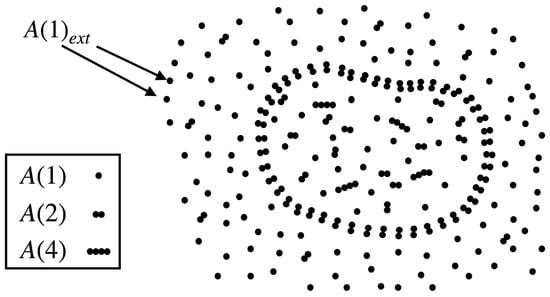
Figure 1.
An illustration of a protocell inside an aqueous medium buffered with monomeric food molecules, . The protocell membrane is composed of dimer molecules .
In this model, the dimer does double duty as both the enclosure-forming molecule as well as a reactant for catalyst production. In the equations below, we do not introduce separate population variables for the two roles. This is purely for simplicity and is not a crucial assumption. In the Supplementary Material, Section 1, we show that in a model with two monomer species in which these two functions are performed by distinct molecules, similar results arise.
Using mass action kinetics, the deterministic rate equations of the model are given by
The terms represent dilution in an expanding volume. Note that when V is not constant, Equations (1)–(3) do not specify the dynamics completely unless the growth rate is specified. Since here we want an endogenous growth rate, we do not specify exogenously. Instead, we write the model in terms of the populations, and assume a certain functional form for V in terms of the populations. In terms of , the above equations reduce to
For simplicity we take V to be a linear function of the populations :
where v is a constant. This choice gives the protocell a constant mass density (as observed in bacterial cells [39]) since V is proportional to the mass of the protocell. This choice is not essential; we have tried other linear functions ( constant), including . The quantitative results depend on the values of but the qualitative features presented below hold for all the cases considered. We have also considered other versions of the model with the transport term in Equation (5) modified to a gradient term (where is the constant concentration of ), certain other autocatalytic reaction topologies, etc. (see Supplementary Material, Section 1). The qualitative conclusions seem to be robust to these choices. Without loss of generality, the constants and v are set to unity by rescaling , , , , and , which makes time and the other parameters dimensionless.
The definition of and the values of the rescaled parameters , and completely define Equations (5)–(7), and one can solve for given any initial condition. In a particular trajectory, V may increase or decrease. Protocells larger than a characteristic size may become floppy or unstable and spontaneously break up into smaller entities. We assume that if V increases to a critical value , the cell divides into two identical daughters, each containing half of the three chemicals of the mother protocell at division. The dynamics of a daughter after division is again governed by Equations (5)–(8). This division rule and Equations (5)–(8) together completely define the model at the deterministic level.
The dynamics of the ACS consisting of the catalyzed reactions R1 and R2 in a fixed-size container but with buffered as the food set is given by Equations (6) and (7), with V and being constant. This was studied in [37] at the deterministic level, where a bistability was observed, and in [38] at the stochastic level, where transitions between the attractors were observed. The present model, by adding Equations (5) and (8) and the division rule, embeds the ACS in a growing–dividing protocell instead of a fixed-volume container. It shares the bistability of the fixed-volume version, but also possesses qualitatively new properties. These properties (considered along with stochastic dynamics) enable a population of such protocells to mimic (one step of) Darwinian evolution, as will be discussed below.
3. Results
3.1. Deterministic Dynamics: Bistability with Two Distinct Growth Rates
Since V is a linear function of the populations, can be expressed in terms of the concentrations. Differentiating Equation (8) with respect to t and using Equations (5)–(7), it follows that
Equation (9) expresses the instantaneous growth rate of the protocell in terms of its chemical composition, a feature that is missing from previous protocell models.
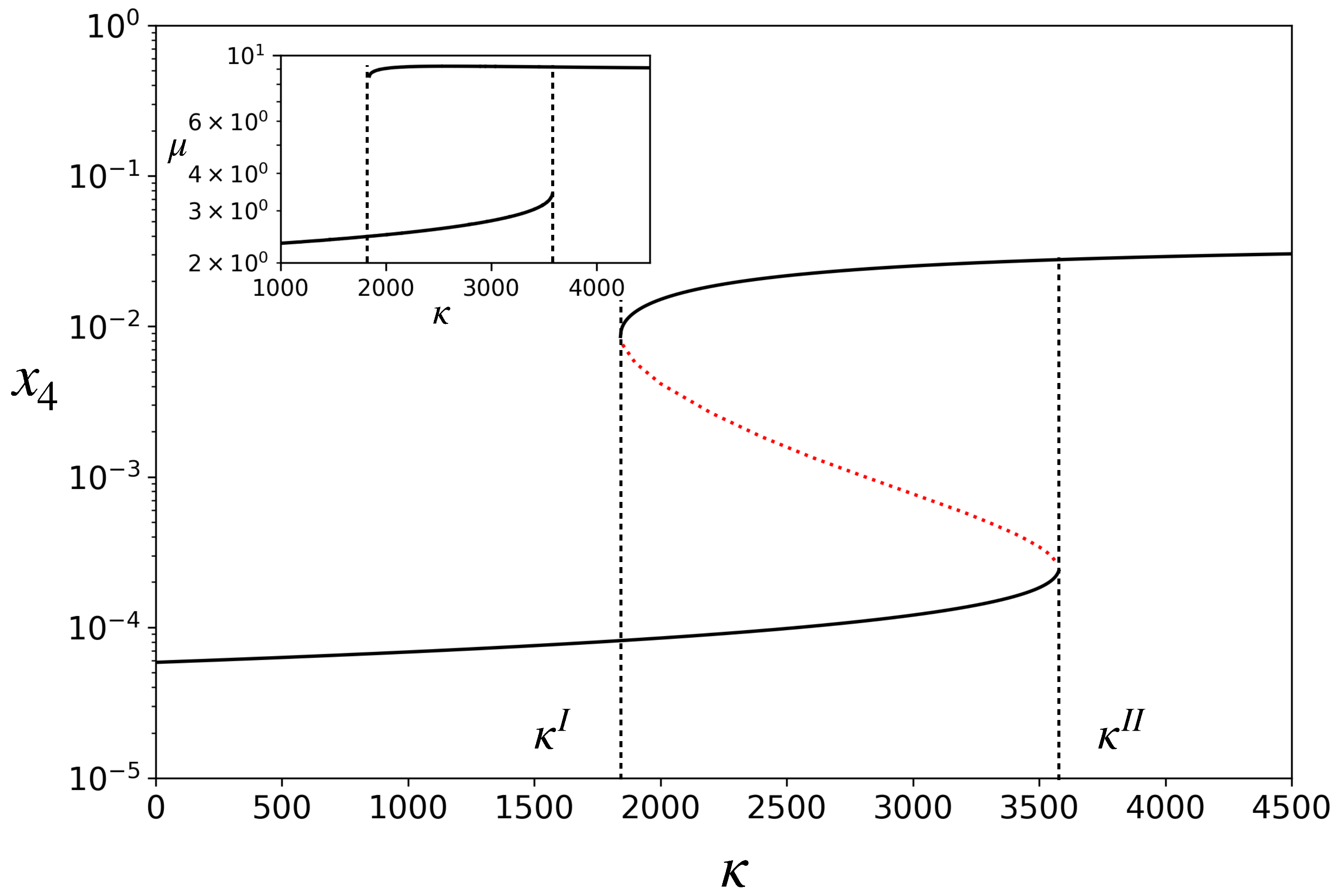
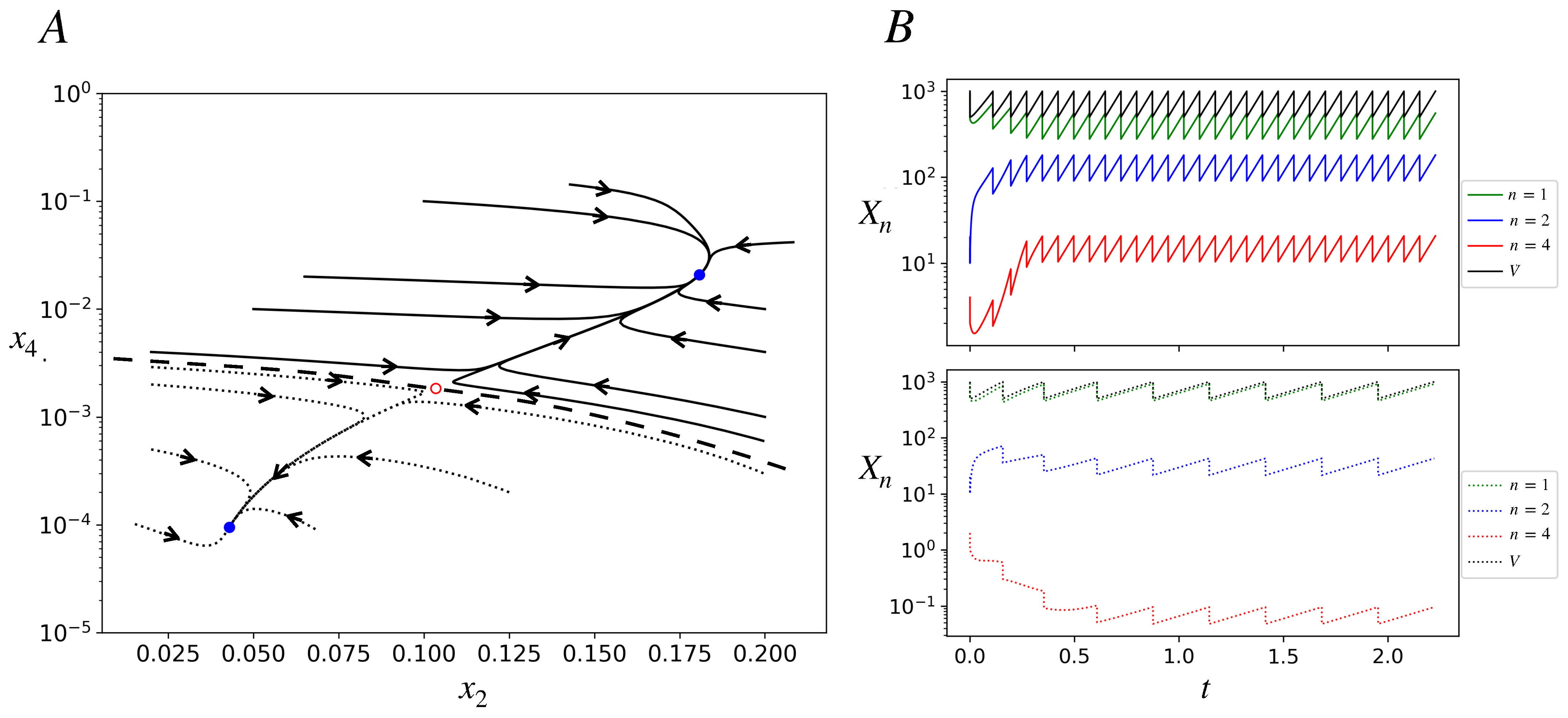
When Equation (9) is substituted into Equations (1)–(3), the concentration dynamics also becomes completely defined. It has fixed points. Figure 2 shows a bifurcation diagram in which the fixed-point concentration of is plotted by varying the parameter . The model exhibits bistability for . Note that the catalyst concentration in the upper stable branch is two orders of magnitude higher than in the lower stable branch. On the lower branch, the rates of catalyzed reactions are smaller than the corresponding spontaneous reactions, while on the upper branch they are much higher. We, therefore, refer to the upper branch as one in which the ACS is active and the lower branch as ACS-inactive. Depending on the initial condition, for a given in the bistable region, the dynamics will settle into either of the two stable attractors, as shown in Figure 3A for one such . For , there is only one attractor (the inactive one), and for , there is also only one attractor (the active one).
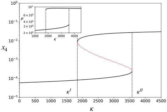
Figure 2.
Bifurcation diagram for the model: steady state concentration, , of the catalyst versus catalytic efficiency, . The region between and is the region having three fixed points, two of which are stable (solid black curves) and one is unstable (red dotted curve). Inset: Growth rate, , of the protocell, versus . Parameters: hereafter, and v have been set to unity without loss of generality after non-dimensionalizing the model. , , .
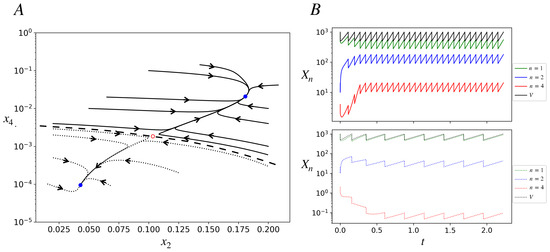
Figure 3.
Deterministic trajectories in the bistable region of the model. ; other parameters are as in Figure 2. The time, t, is in dimensionless units in this figure and subsequent figures (effectively t is measured in units of 1/). (A) Phase portrait projected onto the plane. Several trajectories starting with different initial conditions are shown; they reach one of two stable fixed points denoted by blue closed dots. All the solid curve trajectories end at the stable fixed point on the top right (ACS-active), while all the dotted trajectories end at the stable fixed point on the bottom left of the plot (ACS-inactive). The red open dot represents an unstable fixed point. The dashed curve is a schematic of the basin boundary between the two stable fixed-point attractors. (B) Deterministic trajectories of populations (in log scale) of species , , and and the protocell volume as functions of time for two initial conditions. . Initial conditions: IC1 (lower panel; dotted curves): . IC2 (upper panel; solid curves): . Protocell starting with IC1 ends up in the inactive state, in which the population of the catalyst is less than one, as seen in dotted red curve in the lower panel. Protocell starting with IC2 ends up in the active state, in which the population of the catalyst is high (approximately between 10 and 20). The interdivision times in the inactive and active states are, respectively, , .
For each fixed-point attractor, the right-hand side of Equation (9) is constant. Hence, in the attractor, V grows exponentially, with constant . In other words, the protocell has a characteristic growth rate in each attractor given by the expression in Equation (9). This is shown in the inset of Figure 2. Hence, in the bistable region, the protocell can grow with two distinct growth rates depending upon which attractor it is in. The growth rate is many times higher in the active state than in the inactive one.
Once the concentrations have reached their fixed-point attractor, (9) implies that V grows exponentially, and Equation (8) then implies that each chemical population must also grow exponentially with the same rate, . (Only if all populations grow at the same rate as V will their concentrations be constant). Thus, in each attractor we have . In other words, the protocell naturally exhibits balanced growth in each attractor (growth with ratios of all populations constant [40]). Exponentially growing trajectories in a nonlinear system and this remarkable emergent coordination between the chemicals without any explicit regulatory mechanism are a consequence of (a) the fact that the right-hand sides of Equations (5)–(7) are homogeneous degree-one functions of the populations (if all three populations are simultaneously scaled by a factor , , then the right-hand sides of Equations (5)–(7) also scale by the same factor ), and (b) that the ACS structure couples all chemicals to each other. This is discussed in detail in Ref. [41] in the context of models of bacterial physiology.
Figure 3B shows, for a protocell, the trajectories of its chemical populations and volume as functions of time for two very close initial conditions (defined by the population of species A(1), A(2), and A(4)) that lie in different attractor basins. They converge to different attractors: ACS-active (upper panel) and inactive (lower panel). After a protocell divides we track one of its daughters. The attractor is a fixed point for concentrations (Figure 3A) but a limit cycle for populations and the volume (Figure 3B). The growth phase of the limit cycle has the same constant slope for all populations in a given attractor, signifying exponential growth with the same growth rate for all chemicals in the attractor. The slope is larger (and interdivision time shorter) for the active attractor. At division, since populations and the volume both halve, concentrations do not see any discontinuity.
The existence of bistability is robust in the parameter space. It may be noted that a nonzero degradation rate of the dimer and tetramer is essential for bistability (as also found in the model studied in Ref. [37]). A degradation term for the monomer can also be introduced in Equation (1); however, it is found that must be sufficiently smaller than for bistability to exist.
3.2. Stochastic Dynamics of a Single Protocell: Transitions between States of Different Growth Rates
We now consider the protocell under the stochastic chemical dynamics framework. The chemical populations are now non-negative integers and each unidirectional reaction occurs with a probability that depends on the populations of the reactants and the values of the rate constants. We simulate the stochastic chemical dynamics of the protocell using the Gillespie algorithm [42]. The reaction probabilities are listed in Appendix A. Whenever a reaction occurs, the populations of its reactants and products are updated. For large populations, when fluctuations are ignored, the above-mentioned probabilities lead to the deterministic Equations (1)–(3) or (5)–(7). In using the Gillespie algorithm for expanding volumes, the rate of increase in the volume needs to be taken into account [43,44]. In the present work, since volume is treated as a function of populations (8), we assume that it is instantaneously updated when the populations are.
Figure 4 shows a simulation run of the stochastic chemical dynamics of a single growing and dividing protocell. At the volume threshold , when the protocell divides into two daughter protocells, we implement partitioning stochasticity, namely, each molecule in the mother is given equal probability of going into either daughter. In Figure 4, at each division we randomly discard one of the two daughters and choose one for further tracking, in order to display a single-cell trajectory over several divisions (effectively it is the trajectory of a single lineage of protocells).

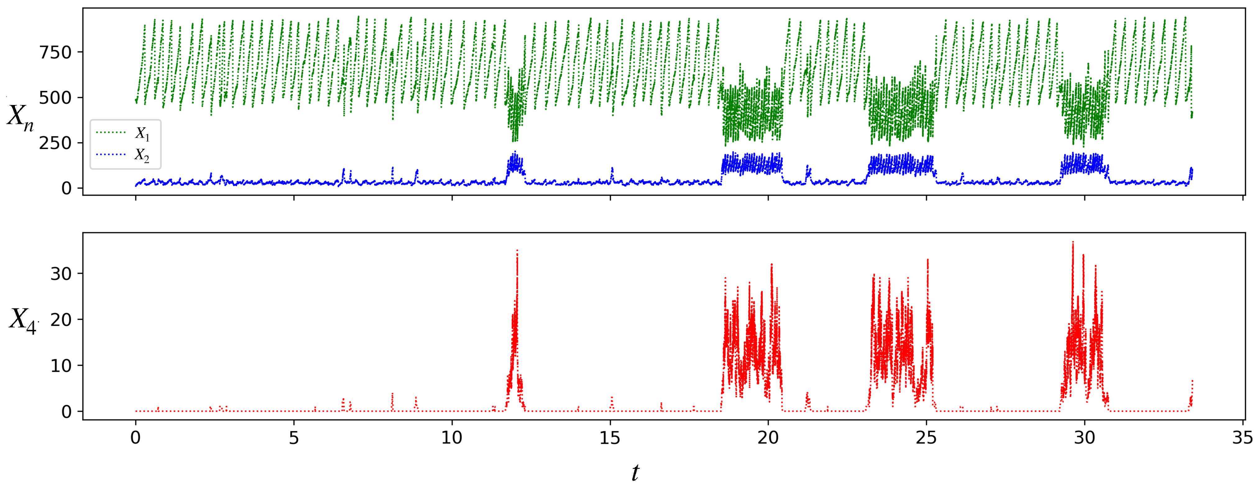
Figure 4.
Stochastic simulation of the populations of species A(1), A(2), and A(4) for a single protocell lineage in the model. Parameter values are as in Figure 3, . Initial condition: . Note the transitions of the protocell between the inactive and active states. From a long such simulation we find that the average interdivision times in the inactive and active states are, respectively, , and , while the average residence times in the two states are , and .
Starting from the initial condition shown, where the protocell is composed of only and , the protocell initially grows and divides in the inactive state. The first molecule is produced by the chance occurrence of the uncatalyzed reaction 2. Production of a sufficient number of molecules triggers a transition to the active state, where the population of is significantly larger than in the inactive state. As in Figure 3 for the deterministic case, so also in Figure 4 it can be seen that the protocell in the active state grows and divides faster than in the inactive state. However, unlike the deterministic case, we also see transitions between the inactive and active states. These transitions occur because for a small protocell ( for the protocell in Figure 4), chance production or depletion of a few molecules of is enough to push its concentration into the basin of the other attractor. Note that in Figure 4, the protocell lineage spends more time in the inactive state than the active. The residence times of a protocell lineage in the two attractors () have distributions (see Figure A1 in Appendix B) that vary with the parameters.
Note that typically a daughter naturally inherits the state of the mother protocell: since the two daughters have roughly half the number of molecules of each type as the mother, and hence also half the volume, they have the same concentration of each chemical as the mother. Partitioning stochasticity occasionally results in a daughter losing the mother’s state.
3.3. Protocell Population Dynamics: Dominance of the Autocatalytic State
Figure 5 shows the time evolution of a population of such protocells. At we start from a single protocell in the inactive state, whose dynamics was shown in Figure 4. However, in this simulation, when a protocell divides, instead of discarding a daughter, we keep it in the simulation until the total population of protocells reaches an externally imposed ceiling K. After the total number of cells reaches K, the total population is kept constant. This is achieved by removing one randomly chosen protocell from among the protocells whenever any protocell divides. Each protocell in the population is independently simulated by the single-cell stochastic dynamics (Gillespie algorithm). Figure 5 tracks only the number of protocells in each state (active or inactive) as a function of time.
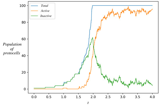
Figure 5.
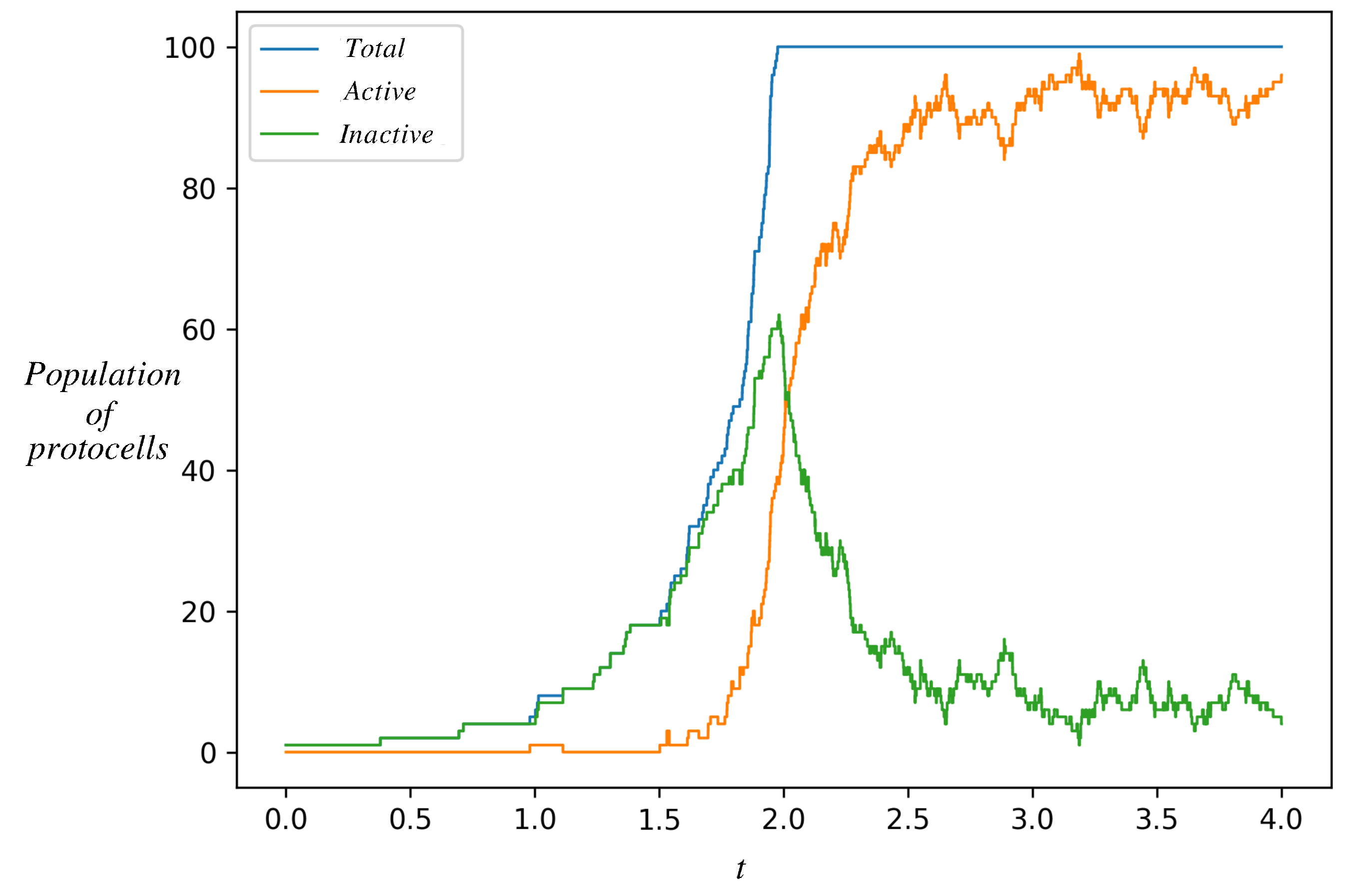
Time evolution of a population of protocells starting from a single protocell in the inactive state. Shown is the number of protocells in the inactive state (green), active state (orange), and their sum (blue). As inactive protocells grow and divide, their population increases. The orange curve departs from zero when one of the inactive protocells makes a stochastic transition to the active state. The two populations have different growth rates. After the total population reaches an externally imposed ceiling K (=100 in this figure), upon each cell division a randomly chosen protocell is removed from the population. The population eventually settles down in a stochastic steady state dominated by the active protocells. This is the natural selection of an autocatalytic state. Parameter values are as in Figure 4, .
The number of protocells in the inactive state increases whenever one of them divides. Eventually, one of them makes a stochastic transition to the active state, whereupon the number of active protocells jumps from zero to one. Active protocells also make stochastic transitions to the non-active state on a certain timescale. However, since active protocells divide faster (as seen in Figure 4), their number grows faster and their population catches up and overtakes the inactive population in Figure 5. Eventually, the active protocells dominate the population.
The curves in Figure 5 represent the net result of stochastic transitions and proliferation by division. The fraction of protocells in each state is expected to reach a stochastic steady state (see below) that represents a balance between proliferation and transition. In the simulations, we find that the fraction of inactive cells declines when the total population hits K (see Figure 5). It eventually reaches its steady state fraction. A decline is seen at the time that the total population hits K, because in this simulation at that time the fraction of inactive cells is higher than its steady state fraction (this is a consequence of the initial condition, the fact that at we started from a single protocell in the inactive state). In Supplementary Material, Section 2, a similar qualitative behavior can be seen for other values of within the bistability region.
An approximate (mean field) model of the protocell population dynamics (valid for large populations) with no ceiling () is the following:
where is the population of protocells in the inactive (active) state, and are the average growth rates of the protocell in the inactive and active states, respectively, and and are the transition rates, respectively, from the inactive to active and active to inactive states. This is a linear dynamical system , where is the column vector of protocell populations, and
Equations (10) and (11) for the populations of inactive and active protocells are identical to the model used to describe the populations of persister and normal cells of bacteria [45].
The steady state fraction f of active protocells in the population can be computed from the eigenvector of A corresponding to its largest eigenvalue, . The result is
where , , and . A calculation of f for a finite but large-ceiling K is given in Appendix C.1 and yields the same answer as (13), independent of K.
Using the averages given in the caption of Figure 4 to determine the components of A, this calculation yields (mean ± standard error), with the error arising from the finite sample estimation of the averages. This agrees with the fraction found (over long times) in the stochastic steady state of the simulation of Figure 5, namely, (mean ± standard deviation). The Supplementary Material, Section 3, shows the agreement between the simulations and the mean-field model at other values of .
Note in Figure 5, that even though the active protocells have a higher growth rate than the inactive, a finite fraction of the inactive still survives in the steady state. This is because of the nonzero transition probability from the active to the inactive state. If had been zero, the eigenvector of A corresponding to its largest eigenvalue would have been , implying that the inactive state is extinct in the steady state. When , one can show (see Appendix C.2) that if
then is close to unity. The quantity defines a certain timescale of the single protocell dynamics. The above condition means that if the average lifetime () of the active state is much larger than this timescale, ACS-active protocells will come to dominate the population. Another way of writing this condition is . Therefore, a sufficient condition for active protocells to dominate is that the active protocell divides many times in its typical lifetime () and grows much faster than the inactive protocell ().
Note also that a nonzero is what ensures that even if we start with a zero population of active protocells, one active protocell will sooner or later be produced by chance, leading eventually to a fraction f of active protocells.
4. Discussion And Conclusions
In this work, we have constructed an example that shows (i) how autocatalytic sets of reactions inside protocells can spontaneously boost themselves into saliency and enhance the populations of their product molecules including catalysts, and (ii) how such protocells (where the ACS is active) can come to dominate in a population of protocells. Encasement within protocells serves two important functions. (i) The small size of a protocell allows a small number fluctuation of the catalyst molecules to take their concentration past the basin boundary of the attractor in which the ACS is inactive into the basin of the active attractor, thereby causing the protocell to transition from an inactive to active state. A large container would require a larger number fluctuation to achieve the same transition, which is more unlikely. (ii) Protocells in the active state grow at a faster rate than the inactive state, thereby eventually dominating in the population. The differential growth rate is a consequence of the fact that the protocell size depends upon its internal chemical populations, a possibility that is precluded when we discuss chemical dynamics in a fixed-size container. Therefore, in this example, protocells aid both the generation and the amplification of autocatalytic sets.
The differential growth rates of the two states are not posited exogenously, but arise endogenously within the model from the underlying chemical dynamics defined by Equations (5)–(8) (and their stochastic version). The additional assumption made is that upon reaching a critical size a protocell divides into two daughters that share its contents. This property can arise naturally due to some physical instability. Collectively these assumptions lead to the properties of heredity, heritable variation (the variation is heritable because once the fluctuation pushes it into a new basin of attraction a protocell typically descends into its new attractor in a short time), and differential fitness in a purely physico-chemical system. This leads to the dynamics of the two subpopulations of protocells shown in Figure 5, which is similar to that of natural selection. (A difference is that the slower-growing subpopulation never goes completely extinct, due to the nonzero probability of the transition of a faster-growing protocell into a slower-growing one).
The process of going from an initial state with no ACS to its establishment in a population of protocells, discussed here, might be considered the first step in the evolution of the ACS. One might wonder how the ACS would evolve further from there. It has been shown that chemistries containing ACSs exhibit multistability in fixed-size containers. In some of these chemistries, simpler ACSs involving small catalyst molecules are nested inside more complex ACSs having larger and more efficient catalyst molecules [37]. The multiple attractor states correspond to ACSs with progressively larger molecules and higher levels of complexity being active. It is possible that by embedding such chemistries within protocells, the mechanism discussed here could allow one to realize a punctuated evolutionary path through sequentially more complex ACS attractors to a state of high chemical complexity from an initial state that only contains small molecules and no ACS. This is a task for the future.
The specific artificial chemistry and protocell properties studied here are highly idealized ones. The object was to demonstrate a mechanism in principle. However, we believe the mechanism is quite general and it should be possible to demonstrate it in other models (e.g., [11,27]) provided multistability in a fixed environment and the emergence of distinct timescales, as discussed in the present work, can be established. We remark that although we have been primarily thinking of protocells as vesicles (motivated by similar models of bacterial physiology), some of our methods might also be useful in the context of micelles. Recently, Kahana et al [31] presented a model of the stochastic dynamics of lipid micelles which had multiple attractors corresponding to distinct composomes. It would be interesting to compare the growth rates of micelles in different attractors as well as the transition rates between the attractors in their model.
We note that there have been independent experimental developments in constructing bistable autocatalytic chemistries [46] and self-replicating protocells [22]. It is also established that small peptides exhibit catalytic properties [47] and they can be encapsulated within protocells to promote protocellular growth [48]. A recent paper also shows the coupling of a simple autocatalytic reaction with the compartment growth and division [49]. A synthesis of these approaches might result in the experimental realization of the mechanism described in the present work.
We have considered dynamics at three levels. One is the chemical dynamics of molecules within a single protocell. This depends upon molecular parameters such as rate constants, the efficiency of the catalyst molecule, etc. From this, we extracted effective parameters at the second level: that of a single protocell (growth rates of the two protocell states, residence times, etc.). These were then used to derive the dynamics at the third level, consisting of the population of protocells. This enabled an understanding of the conditions under which active protocells would dominate. Such an approach might be useful in other settings, for example, in understanding certain aspects of bacterial ecology from molecular models of single bacterial cells.
To conclude, we have shown that in theory, under suitable assumptions, a compartment containing an autocatalytic set of small molecules can self-replicate, produce heritable variation, and evolve in the Darwinian sense to a state of higher complexity. Notably, the model also tells us the conditions required on various timescales for this to happen. This may help in further exploring, both theoretically and experimentally, the evolutionary capabilities of simple molecular systems that precede the origin of life.
Supplementary Materials
The following supporting information can be downloaded at: https://www.mdpi.com/article/10.3390/life13122327/s1, Figure S1: Bifurcation diagram for the 5-chemical-species model; Figure S2: Stochastic simulation of population of species A(1), B(1), A(2), B(2) and A(4) for the model using the Gillespie algorithm; Figure S3: Time evolution of a population of protocells in the 5-chemical-species model starting from a single protocell in the inactive state; Figure S4: Simulations of the model at = 2000; Figure S5: Simulations of the model at = 3400; Figure S6: Fraction f of ‘ACS active’ protocells in the stochastic steady state of the protocell population dynamics versus , obtained from simulation (black hollow circles) and the mean field model (red solid dots).
Author Contributions
Conceptualization, S.J.; methodology, A.Y.S. and S.J.; simulations, A.Y.S.; formal analysis, A.Y.S. and S.J.; investigation, A.Y.S. and S.J.; writing—original draft preparation, A.Y.S. and S.J.; writing—review and editing, A.Y.S. and S.J.; supervision, S.J. All authors have read and agreed to the published version of the manuscript.
Funding
This research was partially supported by the Indo-French Centre for the Promotion of Advanced Research (IFCPAR), project No. 5904-3. AYS would like to thank the University Grants Commission, India, for a Senior Research Fellowship and a Junior Research Fellowship.
Institutional Review Board Statement
Not Applicable.
Informed Consent Statement
Not Applicable.
Data Availability Statement
The data relevant for this work are contained within the article or the supplementary material.
Acknowledgments
We thank Sandeep Krishna, Philippe Nghe, Parth Pratim Pandey, Shagun Nagpal Sethi, Yashika Sethi, and Atiyab Zafar for fruitful discussions. We would like to acknowledge the hospitality of the International Centre for Theoretical Sciences, Bengaluru and the International Centre for Theoretical Physics, Trieste, where part of this work was performed.
Conflicts of Interest
The authors declare no conflict of interest.
Abbreviations
The following abbreviations are used in this manuscript:
| ACS | Autocatalytic set |
Appendix A. Reaction Probabilities Used in Gillespie Algorithm

Table A1.
List of unidirectional reactions in the model and their reaction probabilities per unit time. V appearing in the table is given by the right-hand side of Equation (9) in the main paper text. Deterministic rates of reactions in the last column are given as in Equations (5)–(7) of the main paper.
| Reaction | Reaction Type | Reaction Probability per Unit Time | Deterministic Rate of Reaction |
|---|---|---|---|
| transport | |||
| spontaneous | |||
| catalyzed | |||
| spontaneous | |||
| catalyzed | |||
| spontaneous | |||
| catalyzed | |||
| spontaneous | |||
| catalyzed | |||
| degradation | |||
| degradation |
Appendix B. Single-Cell Residence Time and Interdivision Time Distributions for Active/Inactive States of the Protocell
Appendix B.1. Definition of an Active/Inactive State of a Protocell
In order to obtain residence times and interdivision times in the active and inactive states of the protocell, an inference has to be made from the intracellular populations as to whether the protocell is in the active state or inactive state. The protocell was defined to be in the active (inactive) state if its concentration profile was in the basin of attraction of the active (inactive) attractor. The two basins are separated by a basin boundary (as shown by the black dashed curve in Figure 3A of the main paper). One might choose an alternative criterion based on ‘closeness’ to the attractor state, but for the purposes of the present work, the above definition is useful. In practice, for simplicity in the present work, the concentration of the catalyst molecule () at the unstable fixed point (through which the basin boundary passes) was taken to be the threshold value for determining the state of the protocell. If was above this value, the cell was labeled as active, otherwise it was labeled as inactive. This is an approximate implementation of the above definition. While the actual values of transition times would change when the above definition is implemented exactly, we do not expect our qualitative conclusions to depend significantly on this approximation.
Appendix B.2. Definition of Residence Time and Interdivision Time
While tracking the trajectory of a single lineage of cells (as shown in Figure 4 of the main paper) the state of the protocell (1 if active; 0 if inactive) was determined for the mother protocell at every division along with the time of the division event. (For more details on data generation, see Section 4 of the Supplementary Material). A long such trajectory gave a sequence of division times and a corresponding sequence of ones and zeros. A contiguous subsequence consisting of only ones bordered by zeros (only zeros bordered by ones) at both ends of the subsequence was declared to be an instance of residence in the active state (inactive state). The duration of such a subsequence (equal to the difference between the ending and starting times of the subsequence as measured by the corresponding division times) was taken to be the lifetime of the state. Within an active or inactive subsequence, the difference between two consecutive division times was taken to be an instance of an interdivision time in that state.
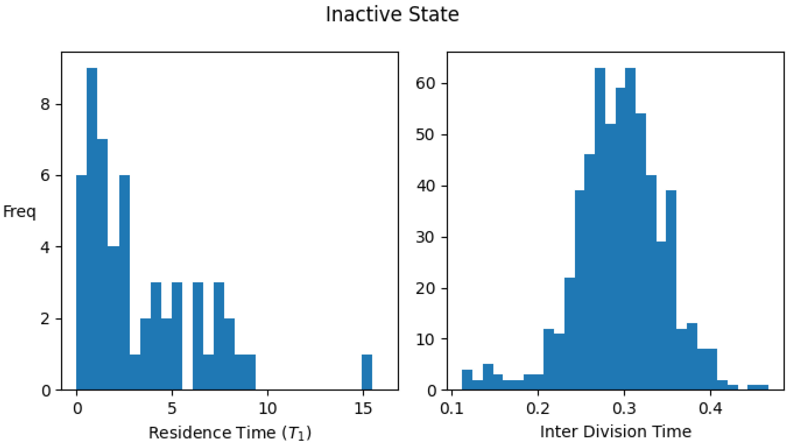
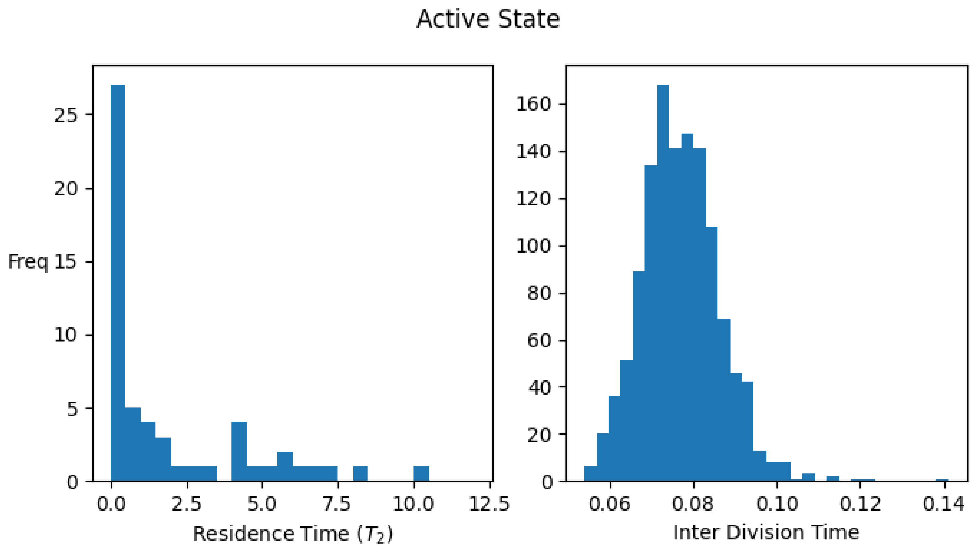
Figure A1 shows the histograms for the residence times and interdivision times in the active and inactive states using the above definitions, for one set of parameter values.

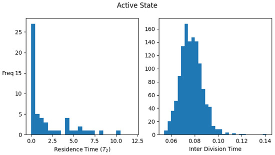
Figure A1.
Distribution of residence times (time spent) and interdivision time in active and inactive states. Data were collected by simulating a single lineage of growing and dividing protocells over 2000 division cycles. Parameter values: . The average values of the interdivision times are and , while the average residence times in the two states are and .
Appendix C. The Steady State Fraction of ACS-Active Protocells (f) in the Protocell Population
An expression was derived for the asymptotic fraction of active protocells in the protocell population dynamics (Equation (13) of the main paper). The derivation used mean-field equations for the populations of the active and inactive protocells and assumed indefinite growth of the two populations. Here, we show that the same expression follows if we truncate the total population of protocells at a large-ceiling K. We analyze the conditions under which this fraction is close to unity. We also present numerical evidence that the fraction so obtained agrees with the actual stochastic simulations of protocell population dynamics at different values of .
Appendix C.1. Calculation of f for a System with Finite-Ceiling K on the Total Population
In our stochastic simulations of protocell population dynamics, the total number of protocells increases until it reaches the ceiling K. After that, it becomes constant because whenever a protocell divides, one protocell chosen at random is removed from the population. Consider the dynamics of and (populations of the inactive and active protocells, respectively) after the total population has reached this constant value K. If K is sufficiently large, we can use the same equations as before (namely, Equations (10) and (11) of the main text) modified by the addition of a death term on the right-hand side. In other words,
where the last term in both equations accounts for the removal of active or inactive protocells in proportion to their existing population (the average effect of the random removal of a protocell from the population). is chosen so that the total population is constant, i.e., . Then, using , we obtain
Eliminating from the equation, and setting to obtain a fixed point, we obtain a quadratic equation for the fixed-point value of :
This has the solution
When is positive (as is the case in our simulations), the positive root must be chosen to obtain a physical solution (non-negative value of ). This yields
The expression of f is independent of K. A bit of algebra shows that this expression is identical to that in Equation (13) of the main paper.
Appendix C.2. Condition for Active Protocells to Dominate the Population
The above expression for f can be written as
where and . This shows that f only depends upon the two dimensionless combinations s and d of the four parameters.
From the above expression, it immediately follows that when , as already mentioned in the main text. We can also ask: How small should be for f to be close to unity? To see this it is useful to introduce the combinations and . Then,
When , the second term inside the square root is much smaller than unity. Performing a Taylor expansion, we obtain to leading order in . This shows that the condition for the active protocells to dominate in the steady state of the population dynamics is
We remark that as a special case, if , then the above condition will hold (since ), and active protocells will dominate. However, the inequality (A9) gives a more general condition for active protocell domination.
References
- Oparin 1924, A.I. Proiskhozhdenie Zhizni (The Origin of Life, Translation by Ann Synge). In The Origin of Life; Bernal, J.D., Ed.; Weidenfeld and Nicolson: London, UK, 1967. [Google Scholar]
- Haldane, J.B.S. Origin of life. Ration. Annu. 1929, 148, 3–10. [Google Scholar]
- Eigen, M. Selforganization of matter and the evolution of biological macromolecules. Naturwissenschaften 1971, 58, 465–523. [Google Scholar] [CrossRef]
- Kauffman, S. Cellular Homeostasis, Epigenesis and Replication in Randomly Aggregated Macromolecular Systems. J. Cybern. 1971, 1, 71–96. [Google Scholar] [CrossRef]
- Rössler, O.E. Ein systemtheoretisches Modell zur Biogenese/A System Theoretic Model of Biogenesis. Z. Für Naturforschung B 1971, 26, 741–746. [Google Scholar] [CrossRef]
- Kauffman, S. The Origins of Order; Oxford University Press: New York, NY, USA, 1993. [Google Scholar]
- Hordijk, W. A History of Autocatalytic Sets. Biol. Theory 2019, 14, 224–246. [Google Scholar] [CrossRef]
- Farmer, J.D.; Kauffman, S.A.; Packard, N.H. Autocatalytic replication of polymers. Phys. D Nonlinear Phenom. 1986, 22, 50–67. [Google Scholar] [CrossRef]
- Bagley, R.; Farmer, J.D.; Fontana, W. Evolution of a metabolism. In Artificial Life II; Langton, C.G., Ed.; Addison-Wesley Publishing Company: Redwood City, CA, USA, 1991; pp. 141–158. [Google Scholar]
- Jain, S.; Krishna, S. Autocatalytic Sets and the Growth of Complexity in an Evolutionary Model. Phys. Rev. Lett. 1998, 81, 5684–5687. [Google Scholar] [CrossRef]
- Vasas, V.; Fernando, C.; Santos, M.; Kauffman, S.; Szathmáry, E. Evolution before genes. Biol. Direct 2012, 7, 1. [Google Scholar] [CrossRef]
- Nghe, P.; Hordijk, W.; Kauffman, S.A.; Walker, S.I.; Schmidt, F.J.; Kemble, H.; Yeates, J.A.M.; Lehman, N. Prebiotic network evolution: Six key parameters. Mol. BioSyst. 2015, 11, 3206–3217. [Google Scholar] [CrossRef]
- Ameta, S.; Matsubara, Y.J.; Chakraborty, N.; Krishna, S.; Thutupalli, S. Self-Reproduction and Darwinian Evolution in Autocatalytic Chemical Reaction Systems. Life 2021, 11, 308. [Google Scholar] [CrossRef]
- Gánti, T. Organization of chemical reactions into dividing and metabolizing units: The chemotons. Biosystems 1975, 7, 15–21. [Google Scholar] [CrossRef]
- Segré, D.; Lancet, D.; Kedem, O.; Pilpel, Y. Graded Autocatalysis Replication Domain (GARD): Kinetic Analysis of Self-Replication in Mutually Catalytic Sets. Orig. Life Evol. Biosph. 1998, 28, 501–514. [Google Scholar] [CrossRef] [PubMed]
- Rasmussen, S.; Chen, L.; Nilsson, M.; Abe, S. Bridging Nonliving and Living Matter. Artif. Life 2003, 9, 269–316. [Google Scholar] [CrossRef]
- Solé, R.V.; Munteanu, A.; Rodriguez-Caso, C.; Macía, J. Synthetic protocell biology: From reproduction to computation. Philos. Trans. R. Soc. B Biol. Sci. 2007, 362, 1727–1739. [Google Scholar] [CrossRef]
- Mavelli, F.; Ruiz-Mirazo, K. Stochastic simulations of minimal self-reproducing cellular systems. Philos. Trans. R. Soc. B Biol. Sci. 2007, 362, 1789–1802. [Google Scholar] [CrossRef] [PubMed]
- Carletti, T.; Serra, R.; Poli, I.; Villani, M.; Filisetti, A. Sufficient conditions for emergent synchronization in protocell models. J. Theor. Biol. 2008, 254, 741–751. [Google Scholar] [CrossRef] [PubMed]
- Kamimura, A.; Kaneko, K. Reproduction of a Protocell by Replication of a Minority Molecule in a Catalytic Reaction Network. Phys. Rev. Lett. 2010, 105, 268103. [Google Scholar] [CrossRef] [PubMed]
- Hordijk, W.; Naylor, J.; Krasnogor, N.; Fellermann, H. Population Dynamics of Autocatalytic Sets in a Compartmentalized Spatial World. Life 2018, 8, 33. [Google Scholar] [CrossRef]
- Luisi, P. The Emergence of Life: From Chemical Origins to Synthetic Biology; Cambridge University Press: Cambridge, UK, 2016. [Google Scholar]
- Serra, R.; Villani, M. Modelling Protocells: The Emergent Synchronization of Reproduction and Molecular Replication; Understanding Complex Systems; Springer: Dordrecht, The Netherlands, 2017. [Google Scholar]
- Lewontin, R.C. The Units of Selection. Annu. Rev. Ecol. Syst. 1970, 1, 1–18. [Google Scholar] [CrossRef]
- Godfrey-Smith, P. Conditions for Evolution by Natural Selection. J. Philos. 2007, 104, 489–516. [Google Scholar] [CrossRef]
- Segré, D.; Ben-Eli, D.; Lancet, D. Compositional genomes: Prebiotic information transfer in mutually catalytic noncovalent assemblies. Proc. Natl. Acad. Sci. USA 2000, 97, 4112–4117. [Google Scholar] [CrossRef]
- Villani, M.; Filisetti, A.; Graudenzi, A.; Damiani, C.; Carletti, T.; Serra, R. Growth and Division in a Dynamic Protocell Model. Life 2014, 4, 837–864. [Google Scholar] [CrossRef] [PubMed]
- Serra, R.; Villani, M. Sustainable Growth and Synchronization in Protocell Models. Life 2019, 9, 68. [Google Scholar] [CrossRef]
- Togashi, Y.; Kaneko, K. Transitions Induced by the Discreteness of Molecules in a Small Autocatalytic System. Phys. Rev. Lett. 2001, 86, 2459–2462. [Google Scholar] [CrossRef] [PubMed]
- Serra, R.; Filisetti, A.; Villani, M.; Graudenzi, A.; Damiani, C.; Panini, T. A stochastic model of catalytic reaction networks in protocells. Nat. Comput. 2014, 13, 367–377. [Google Scholar] [CrossRef]
- Kahana, A.; Segev, L.; Lancet, D. Attractor dynamics drives self-reproduction in protobiological catalytic networks. Cell Rep. Phys. Sci. 2023, 4, 101384. [Google Scholar] [CrossRef]
- Hordijk, W.; Steel, M. Detecting autocatalytic, self-sustaining sets in chemical reaction systems. J. Theor. Biol. 2004, 227, 451–461. [Google Scholar] [CrossRef]
- Blokhuis, A.; Lacoste, D.; Nghe, P. Universal motifs and the diversity of autocatalytic systems. Proc. Natl. Acad. Sci. USA 2020, 117, 25230–25236. [Google Scholar] [CrossRef]
- Ohtsuki, H.; Nowak, M.A. Prelife catalysts and replicators. Proc. R. Soc. B Biol. Sci. 2009, 276, 3783–3790. [Google Scholar] [CrossRef] [PubMed]
- Wu, M.; Higgs, P.G. Origin of Self-Replicating Biopolymers: Autocatalytic Feedback Can Jump-Start the RNA World. J. Mol. Evol. 2009, 69, 541–554. [Google Scholar] [CrossRef]
- Piedrafita, G.; Montero, F.; Morán, F.; Cárdenas, M.L.; Cornish-Bowden, A. A Simple Self-Maintaining Metabolic System: Robustness, Autocatalysis, Bistability. PLoS Comput. Biol. 2010, 6, 1–9. [Google Scholar] [CrossRef]
- Giri, V.; Jain, S. The Origin of Large Molecules in Primordial Autocatalytic Reaction Networks. PLoS ONE 2012, 7, 1–18. [Google Scholar] [CrossRef] [PubMed]
- Matsubara, Y.J.; Kaneko, K. Optimal size for emergence of self-replicating polymer system. Phys. Rev. E 2016, 93, 032503. [Google Scholar] [CrossRef]
- Martínez-Salas, E.; Martín, J.A.; Vicente, M. Relationship of Escherichia coli density to growth rate and cell age. J. Bacteriol. 1981, 147, 97–100. [Google Scholar] [CrossRef] [PubMed]
- Campbell, A. Synchronization of cell division. Bacteriol. Rev. 1957, 21, 263–272. [Google Scholar] [CrossRef] [PubMed]
- Pandey, P.P.; Singh, H.; Jain, S. Exponential trajectories, cell size fluctuations, and the adder property in bacteria follow from simple chemical dynamics and division control. Phys. Rev. E 2020, 101, 062406. [Google Scholar] [CrossRef]
- Gillespie, D.T. A general method for numerically simulating the stochastic time evolution of coupled chemical reactions. J. Comput. Phys. 1976, 22, 403–434. [Google Scholar] [CrossRef]
- Lu, T.; Volfson, L.; Tsimring, L.; Hasty, J. Cellular growth and division in the Gillespie algorithm. Syst. Biol. 2004, 1, 121–128. [Google Scholar] [CrossRef]
- Carletti, T.; Filisetti, A. The Stochastic Evolution of a Protocell: The Gillespie Algorithm in a Dynamically Varying Volume. Comput. Math. Methods Med. 2012, 2012, 423627. [Google Scholar] [CrossRef]
- Balaban, N.Q.; Merrin, J.; Chait, R.; Kowalik, L.; Leibler, S. Bacterial Persistence as a Phenotypic Switch. Science 2004, 305, 1622–1625. [Google Scholar] [CrossRef] [PubMed]
- Maity, I.; Wagner, N.; Mukherjee, R.; Dev, D.; Peacock-Lopez, E.; Cohen-Luria, R.; Ashkenasy, G. A chemically fueled non-enzymatic bistable network. Nat. Commun. 2019, 10, 4636. [Google Scholar] [CrossRef] [PubMed]
- Gorlero, M.; Wieczorek, R.; Adamala, K.; Giorgi, A.; Schininà, M.E.; Stano, P.; Luisi, P.L. Ser-His catalyses the formation of peptides and PNAs. FEBS Lett. 2009, 583, 153–156. [Google Scholar] [CrossRef] [PubMed]
- Adamala, K.; Szostak, J.W. Competition between model protocells driven by an encapsulated catalyst. Nat. Chem. 2013, 5, 495–501. [Google Scholar] [CrossRef]
- Lu, H.; Blokhuis, A.; Turk-MacLeod, R.; Karuppusamy, J.; Franconi, A.; Woronoff, G.; Jeancolas, C.; Abrishamkar, A.; Loire, E.; Ferrage, F.; et al. Small-molecule autocatalysis drives compartment growth, competition and reproduction. Nat. Chem. 2023. [Google Scholar] [CrossRef]

Disclaimer/Publisher’s Note: The statements, opinions and data contained in all publications are solely those of the individual author(s) and contributor(s) and not of MDPI and/or the editor(s). MDPI and/or the editor(s) disclaim responsibility for any injury to people or property resulting from any ideas, methods, instructions or products referred to in the content. |
© 2023 by the authors. Licensee MDPI, Basel, Switzerland. This article is an open access article distributed under the terms and conditions of the Creative Commons Attribution (CC BY) license (https://creativecommons.org/licenses/by/4.0/).