Identification of Robot Joint Torsional Stiffness Based on the Amplitude of the Frequency Response of Asynchronous Data

Abstract

The difficulty of adding external excitation and the asynchronous data collection from the industrial robot operation limited the online parameter identification of industrial robots. In this regard, this study proposes an identification method that only uses the amplitude of the frequency response function (FRF) of the system to identify robot joint torsional stiffness and dynamic parameters. The error criterion function shows that this method is feasible and comparable to applying the complete frequency response for identification. The Levenberg–Marquardt (L-M) algorithm is used to find the global optimal value of the error criterion function. In addition, an operational excitation method is proposed to excite the system. The speed profile is set as a triangle wave to excite the system using rectangular wave electromagnetic torques. The simulation results show that using the amplitude of the FRF to identify parameters applies to asynchronous data. The experiments on a single-degree-of-freedom articulated arm test bench show that the motion excitation method is effective, and both stiffness and inertia are identifiable.

1. Introduction

Servo systems have become wildly used with the development of industry and technology, particularly in high-end medical equipment, new energy, robots, CNC machine tools, and other fields [1,2]. Due to the fatigue of the mechanical part of the actual system, the stiffness of the shaft system declines, and the performance of the transmission mechanism reduces as the running time increases. Thus, the introduction of greater motion error in the system is inevitable [3,4]. Therefore, changes in the shaft system stiffness can reflect the operating status of the system and are essential indicators of the performance evaluation and prediction of the transmission system [5,6,7]. Identifying the stiffness of the shaft system during operation is crucial to predict an early failure of an industrial robot [8].

Parameter identification is typically used to estimate the parameters of a mathematical model based on the input and output information of a particular system [9]. The parameter identification in the servo drive system includes two aspects: internal parameter identification and external parameter identification [10,11]. For the dual inertia system with nonlinear characteristics, Beineke [12] proposed two identification methods for external mechanical parameters: standard minimum root mean square and four-step instrumental variable method. They extracted the speed response of the motor at different stages for the dual inertia system with nonlinear characteristics and identified the parameters corresponding to each stage. The identification results were compared with the traditional neural network, self-organizing mapping, and classic frequency domain analysis methods. Villwock and Pacas [13,14] proposed a non-parametric identification method to obtain the resonant frequency of the dual inertia elastic system directly. In the identification process, the pseudo-random binary signal (PRBS) signal was used as an additional disturbance of the stator current to excite the system, while the Welch method was used to obtain frequency response. The measurement results showed that Welch method was extraordinarily suitable for identification. The research of a three-mass-system pointed out that the proposed identification method could resoundingly be applied to complex mechanical systems. Zoubek and Pacas [15] calculated the FRF by implementing an adaptive speed observer to replace the actual encoder. The proposed method could reliably identify various dual inertia systems. However, the identification result could be affected by factors such as time-varying speed and load. In the field of robot parameter identification, Zha et al. [16] proposed RLS-PSO algorithm combining Recursive Least Squares (RLS) and Particle Swarm Optimization (PSO) for the parameter identification of lower limb exoskeleton with emphasis on nonlinear mathematical model. RLS was used to define the search space of each parameter, and then PSO was used to perform iterative optimization in the defined search space. This method could eliminate the potential local minimum as much as possible and improved the identification accuracy of parameters. Ostring [17] analyzed the direct parameter identification method relying on three-inertia modeling for the joints of the ABB IRB 1400 industrial robot. And compared the results with a “black box” model structure identification method. It was found that the three-inertia model could describe the dynamics of the robot well. Urrea [18] identified the dynamic parameters of three-degree-of-freedom manipulator by using the parameter identification algorithms of Least Square (LS), extended Kalman filter, Adaptive Linear Neuron (Adaline) neural networks, Hopfield recurrent neural networks, and genetic algorithms, respectively. The results showed that the LS method and Adaline method have the advantages of less iterations, short calculation time, and high accuracy.

A major inconvenience for parameter identification is asynchronous input and output signals for a servo drive system. Electromagnetic torque and motor speed are used as input and output signals for the identification. The torque can be calculated from the line current, which is analog, while the speed from the motor encoder can be obtained during operation, which is digital. Thus, it is challenging to acquire the two signals synchronously. In addition, the phase of the FRF is coupled with the acquisition time delay, affecting the outcome of the identification process. Therefore, it is worth studying to accurately identify the system parameters under the condition of asynchronous data.

In the system identification process, the selection of the excitation signal is crucial. Bazanellaa [19] pointed out that the amount of information required for identification depends on the amount of information with the closed-loop internal feedback of the actual system and the amount of information added to the data. The external multi-frequency signal (such as PRBS excitation signals) could make the system complete accurate identification in a short time, but it was not a necessary condition for successful identification. In addition, adding an excitation signal to the operational servo mechanical system will cause the system to run unstable and affect its working state.

The traditional identification method of frequency domain uses the FRF for identification, which is only suitable for synchronous data. In addition, the traditional method depends on the external excitation signal, which is difficult to implement in the operation of an industrial robot. In order to evaluate the rigidity of the joint servo system of industrial robots in operation, the identification of the system shaft stiffness under the condition of operational excitation and asynchronous sampling of input and output is studied. An identification method based on the amplitude of the FRF is proposed, and an operational excitation method is used to excite the system. This research provides a valuable reference for condition monitoring of the joint in actual industrial applications.

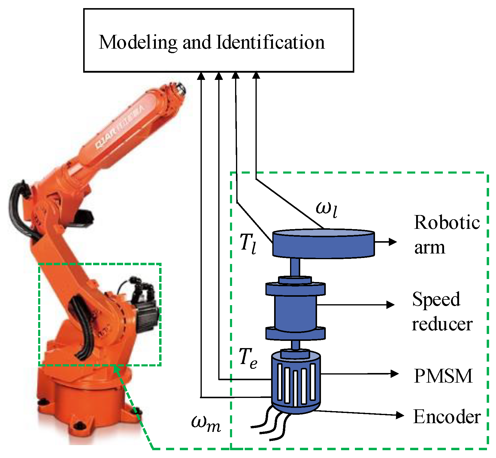
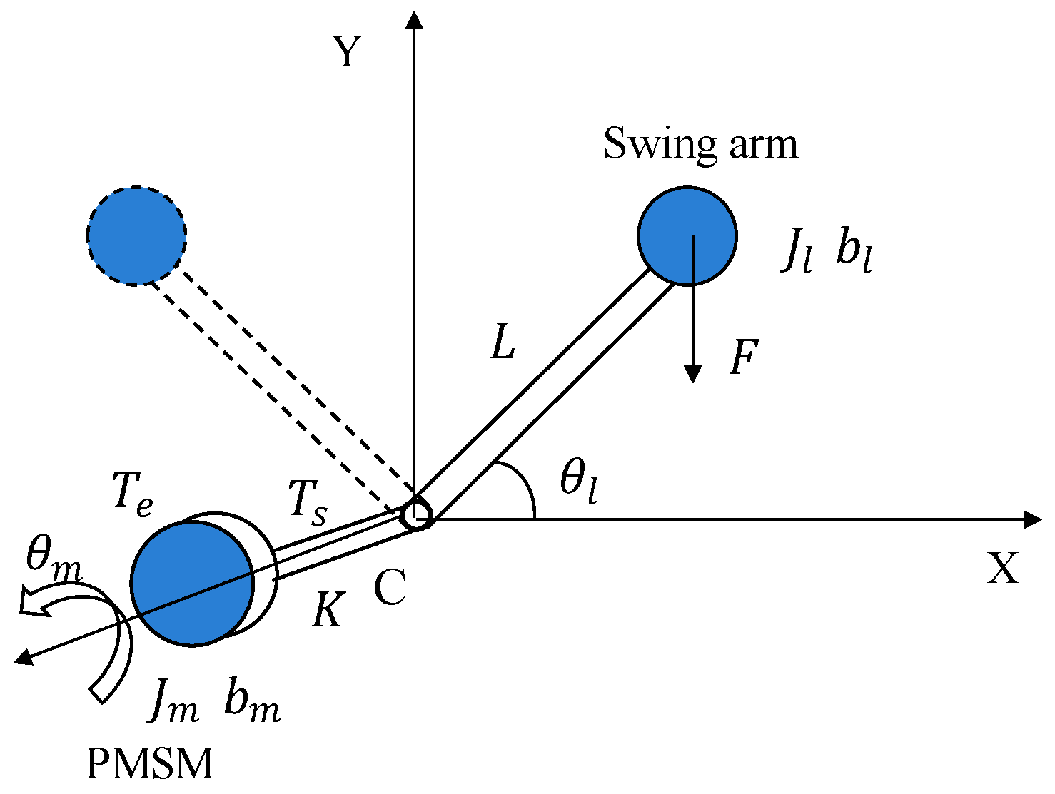
2. Dynamic Modeling of the Robot Joint with Single Degree of Freedom

In this study, only one axis motion of the industrial robot is considered. The typical industrial robot joint is composed of a permanent magnet synchronous motor (PMSM), a speed reducer, and an arm, as shown in Figure 1. In the figure, $T_e$ is electromagnetic torque, ${\omega }_m$ is motor speed, $T_l$ is the load torque, and ${\omega }_l$ is the rotating speed of the articulated arm.

The joint structure of the robot is complex. Moreover, identifying each structural parameter is challenging. However, a robot joint can be equivalent to an identifiable dual inertia model. Equations (1) and (2) can be used to calculate the equivalent stiffness and equivalent load inertia of the joint.

$$K=\frac{1}{\frac{1}{K_1}+\frac{1}{K_2}\dots +\frac{1}{K_n}}$$

(1)

$$J_l=\frac{J_L}{i^2}$$

(2)

where $K_1,K_2,\cdot \cdot \cdot ,K_n$ are the stiffness of each part, or a series of parts, of the shaft. $K$ is the equivalent joint stiffness. $J_L$ and $J_l$ are the actual load inertia and equivalent load inertia, respectively. $i$ is the reduction ratio.

The double inertia model of the system can be obtained, as shown in Figure 2.

The mechanical dynamics of the system can be written as follows:

$$\left.\begin{array}{l}{J}_m{\stackrel{\mathrm{..}}{\theta }}_m +b_m{\stackrel{.}{\theta }}_m=T_e-T_s,\\ J_l{\stackrel{\mathrm{..}}{\theta }}_l +b_l{\stackrel{.}{\theta }}_l=T_s-T_l,\\ T_s=K\left({\theta }_m-{\theta }_l\right) + C({\stackrel{.}{\theta }}_m-{\stackrel{.}{\theta }}_l),\\ {\omega }_m={\stackrel{.}{\theta }}_m,\\ {\omega }_l={\stackrel{.}{\theta }}_l,\\ T_l=FL\cos {\theta }_l\end{array}\right\}$$

(3)

where $J_m$ is the moment of inertia of the servo motor. $b_m$ and $b_l$ are the damping of the motor and the swing, respectively. ${\theta }_m$ and ${\theta }_l$ are the position angle of the motor shaft and articulated arm, respectively. $T_s$ is the shaft torque, $C$ is the damping of the shaft, $F$ is the gravity of the swing arm, and $L$ is the distance from the shaft to the line of action of the load.

According to Equation (3), the transfer function from the electromagnetic torque to motor speed can be obtained as follows:

$$H(s)=\frac{{\omega }_m}{T_e}=\frac{J_l{s}^2+(C+b_l)s+K}{\begin{array}{l}{J}_m{J}_l{s}^3+(J_{m}C+J_{l}C+J_l{b}_m+J_m{b}_l)s^2+\\ (J_{m}K+J_{l}K+C{b}_m+C{b}_l+b_m{b}_l)s+K(b_m+b_l)\end{array}}$$

(4)

Equation (4) shows that the motor speed feedback introduces conjugate zeros and conjugate poles to the closed-loop system, which will lead to mechanical resonance. Through the conjugate zeros and the conjugate pole presented in Equation (4), the anti-resonance frequency (ARF) ${\omega }_{ARF}$ and the natural torsional frequency (NTF) ${\omega }_{NTF}$ can be derived. If $b_m=0$, $b_l=0$, and $C=0$ are assumed, the ${\omega }_{ARF}$ and ${\omega }_{NTF}$ can be expressed as follows:

$${\omega }_{ARF}=\sqrt{\frac{K}{J_l}}$$

(5)

$${\omega }_{NTF}=\sqrt{\frac{(J_m+J_l)K}{J_l{J}_m}}$$

(6)

Since the value of inertia changes by a very small amount in the long-time operation, the stiffness determines the change of the resonance frequencies of the system.

3. Proposed Parameter Identification Method

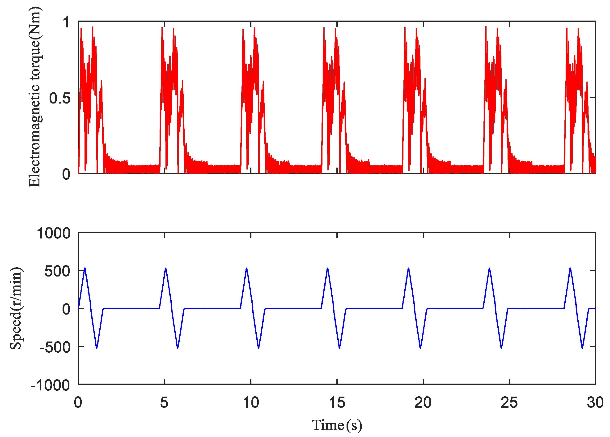
3.1. The Excitation Signal of the Swing Movement

The direct closed-loop identification setup shown in Figure 3 is considered, where $C(s)$ is the linear transfer function of the controller, $P(s)$ is the transfer function of the drive system, $u\left(t\right)$ is the system input, and $y\left(t\right)$ is the system output. ${\omega }_r$ is the reference rotating speed. The novelty of the identification setup is that it does not use external excitation signal because it uses operational excitation.

The identification accuracy depends heavily on the excitation signal, which should cover the frequency components contained in the system. The most used excitation signals are swept-frequency signals and PRBS [20,21]. The excitation signal is superimposed on the torque reference obtained from the speed controller as the input signal to excite the system. However, if the frequency band of the torque itself is wide enough, and the signal strength in the frequency band is large enough, the system can also be excited. Therefore, we considered the electromagnetic torque generated by the reciprocating motion of industrial robots as system’s excitation.

The commonly used speed profile of reciprocating motion of robot joints is the trapezoidal curve. The trapezoidal curve divides the entire movement process into three stages: constant acceleration, constant speed, and constant deceleration [22]. When the motion period is short and the maximum speed is not reached, the trapezoidal curve becomes a triangular wave. For this case, the electromagnetic torque corresponds to a rectangular wave. The frequency spectrum of a rectangular wave is wideband, which can achieve a similar effect to the external excitation.

3.2. Calculation of the Electromagnetic Torque

Torque sensors cannot be implemented to measure torque in industrial robot joints. Thus, the electromagnetic torque is typically calculated from the line current. In this regard, it is necessary to perform a coordinate transformation in the alternating current (AC) motor physical model to obtain the relationship between the electromagnetic torque and the line current [23].

Coordinate transformation follows the principle of constant power before and after transformation, mainly including the following two forms:

(1)

Clarke transformation can be written as follows:

$$\left[\begin{array}{c}{i}_{\alpha }\\ i_{\beta }\end{array}\right]=\sqrt{\frac{2}{3}}\left[\begin{array}{c}\begin{array}{ccc}1& -\frac{1}{2}& -\frac{1}{2}\end{array}\\ \begin{array}{ccc}0& \frac{\sqrt{3}}{2}& -\frac{\sqrt{3}}{2}\end{array}\end{array}\right]\left[\begin{array}{c}{i}_A\\ i_B\\ i_C\end{array}\right]=C_{3s/2s}\left[\begin{array}{c}{i}_A\\ i_B\\ i_C\end{array}\right]$$

(7)

(2)

Park transformation can be written as follows:

$$\left[\begin{array}{c}{i}_d\\ i_q\end{array}\right]=\left[\begin{array}{cc}\cos \theta & \sin \theta \\ -\sin \theta & \cos \theta \end{array}\right]\left[\begin{array}{c}{i}_{\alpha }\\ i_{\beta }\end{array}\right]=C_{2s/sr}\left[\begin{array}{c}{i}_{\alpha }\\ i_{\beta }\end{array}\right]$$

(8)

where $i_A$, $i_B$, $i_C$ are three-phase alternating currents. $i_{\alpha }$ and $i_{\beta }$ are two-phase alternating current in the two-phase stationary coordinate system $\alpha \beta$. $i_d$ and $i_q$ are two direct currents in the two-phase rotating coordinate system $dq$. $C_{3s/2s}$ is the Clarke transformation matrix, while $C_{2s/2r}$ is the Park transformation matrix. $\theta$ represents the electrical angle.

After the coordinate transformation, the decoupling of torque components is performed, and the PMSM mathematical model in the $dq$ coordinate system is obtained. The torque equation can be written as follows:

$$T_e=\frac{3}{2}p\left[{\phi }_d{i}_q-{\phi }_q{i}_d\right]$$

(9)

If $i_d$ is controlled to be zero, PMSM is decoupled, and the torque of PMSM can be written as follows [24,25]:

$$T_e=k_t{i}_q$$

(10)

where ${\phi }_d$ and ${\phi }_q$ are the $d$ and $q$ axis components of the stator flux linkage, $p$ is the number of pole pairs, and $k_t$ is the torque constant.

For $i_d=0$, $i_q$ is equal to the peak value of the line current [26]. As the load torque varies with the position angle, the peak of the line current varies accordingly. As the line current is an analytical signal, its peak curve can be detected as the envelope using Hilbert transform (HT). The modulus of the analyzed signal is the instantaneous amplitude or envelope of the signal [27].

Assuming that the measured line current is $i_a\left(t\right)$, and its HT is denoted as $h\left[i_a\left(t\right)\right]$, then $i_q(t)$ and $T_e(t)$ can be obtained as follows:

$$i_q(t)=\left|h\left[i_a\left(t\right)\right]\right|=\left|\frac{1}{\pi }{\displaystyle {\mathsf{\int }}_{-\infty }^{\infty }\frac{i_a(\tau )}{t-\tau }d\tau }\right|$$

(11)

$$T_e(t)=k_t{i}_q(t)$$

(12)

3.3. Error Criterion Function of the Identification Method of the Amplitude of the FRF

In the operation of the industrial robot, it is difficult for conventional signal acquisition cards to meet the sampling rate requirements when analog sampling is used due to the high accuracy of the encoder. A better way to obtain the speed is to read the encoder data from the driver. This type of signal is digital, which is different from the signal type of current. Thus, the input and the output data are asynchronous, causing deviations in the phase-frequency characteristics of the system, which makes it impossible to identify the system accurately by frequency response. However, the amplitude-frequency characteristics are not affected; therefore, this study proposes a method for parameter identification using the amplitude of the FRF. The following analyzes the identification performance of this method.

In direct closed-loop identification setups, the transfer function in Equation (4) can also be written as follows:

$$\frac{y(s)}{u(s)}=\frac{b_1{s}^2+b_{2}s+b_3}{s^3+a_1{s}^2+a_{2}s+a_3}$$

(13)

where

$$\left\{\begin{array}{l}{b}_1=\frac{1}{J_m}\hfill \\ b_2=\frac{C + b_l}{J_m{J}_l}\hfill \\ b_3=\frac{K}{J_m{J}_l}\hfill \\ a_1=\frac{\left(J_m + J_l\right)C + J_l{b}_m + J_m{b}_l}{J_m{J}_l}\hfill \\ a_2=\frac{\left(J_m + J_l\right)K + \left(b_m + b_l\right)C + b_m{b}_l}{J_m{J}_l}\hfill \\ a_3=\frac{K\left(b_m + b_l\right)}{J_m{J}_l}\hfill \end{array}\right.$$

(14)

The corresponding FRF is

$$H(\omega )=\frac{\left(b_3-b_1{\omega }^2\right) + j{b}_2\omega }{\left(a_3-a_1{\omega }^2\right) + j\left(a_2\omega -{\omega }^3\right)}=\frac{R_1(\omega )+I_1(\omega )j}{R_2(\omega )+I_2(\omega )j}$$

(15)

When using the FRF for identification, the error between the frequency response estimate $\stackrel{\wedge }{H}\left(\omega \right)$ and the actual frequency response $H\left(\omega \right)$ is

$$e\left(\omega \right) =\stackrel{\wedge }{H}\left(\omega \right)-H\left(\omega \right) =R_e(\omega )+I_m\left(\omega \right)j-\frac{R_1(\omega )+I_1(\omega )}{R_2(\omega )+I_2(\omega )}$$

(16)

The generalized error criterion function can be written as follows:

$$E_w={{\displaystyle \sum _{i=1}^N‖e_w\left({\omega }_i\right)‖}}^2={{\displaystyle \sum _{i=1}^N‖\left[R_2\left({\omega }_i\right) + I_2\left({\omega }_i\right)j\right]e\left({\omega }_i\right)‖}}^2$$

(17)

The function can be written further as

$$E_w={\displaystyle \sum _{i=1}^N\left\{\begin{array}{l}{\left[R_e({\omega }_i)R_2({\omega }_i)-I_m({\omega }_i)I_2({\omega }_i)-R_1({\omega }_i)\right]}^2+\\ {\left[R_e({\omega }_i)I_2({\omega }_i)+I_m({\omega }_i)R_2({\omega }_i)-I_1({\omega }_i)\right]}^2\end{array}\right\}}$$

(18)

Equation (18) makes the error criterion function linear with respect to the parameter space, which simplifies the solution of the parameters. Supposing that a parameter $b_1$ minimizes the error criterion function, the partial derivative of the error criterion function with respect to $b_1$ is zero.

$$\frac{\partial E_w}{\partial b_1}=2{\omega }_i{}^2\left[R_e(a_3-a_1{\omega }_i{}^2)-I_m(a_2{\omega }_i-{\omega }_i{}^3)-b_3+b_1{\omega }_i{}^2\right]=0$$

(19)

$$b_1=\frac{b_3-\left[R_e(a_3-a_1{\omega }_i{}^2)-I_m(a_2{\omega }_i-{\omega }_i{}^3)\right]}{{\omega }_i{}^2}$$

(20)

When only the amplitude of the FRF is used for identification, the amplitude of the FRF estimate $\left|\stackrel{\wedge }{H}\left(\omega \right)\right|$ and the actual amplitude of the FRF $\left|H\left(\omega \right)\right|$ should be equal in the absence of error.

$$\left|\stackrel{\wedge }{H}\left(\omega \right)\right|-\left|H\left(\omega \right)\right|=\sqrt{R_e{(\omega )}^2+I_m{\left(\omega \right)}^2}-\frac{\sqrt{R_1{(\omega )}^2+I_1{(\omega )}^2}}{\sqrt{R_2{(\omega )}^2+I_2{(\omega )}^2}}=0$$

(21)

Moreover,

$$\begin{array}{l}\sqrt{{\left[R_e(\omega )R_2(\omega )\right]}^2+{\left[I_m(\omega )I_2(\omega )\right]}^2+{\left[R_e(\omega )I_2(\omega )\right]}^2+{\left[I_m(\omega )R_2(\omega )\right]}^2}\\ =\sqrt{R_1{(\omega )}^2+I_1{(\omega )}^2}\end{array}$$

(22)

Squaring both sides simultaneously

$$\begin{array}{l}{\left[R_e(\omega )R_2(\omega )\right]}^2+{\left[I_m(\omega )I_2(\omega )\right]}^2+{\left[R_e(\omega )I_2(\omega )\right]}^2+{\left[I_m(\omega )R_2(\omega )\right]}^2\\ =R_1{(\omega )}^2+I_1{(\omega )}^2\end{array}$$

(23)

The root of the error function is removed by considering the error. The generalized error criterion function can be written as follows:

$$E_a={\displaystyle \sum _{i=1}^N\left\{\begin{array}{l}{\left({\left[R_e({\omega }_i)R_2({\omega }_i)\right]}^2+{\left[I_m({\omega }_i)I_2({\omega }_i)\right]}^2-R_1{({\omega }_i)}^2\right)}^2+\\ {\left({\left[R_e({\omega }_i)I_2({\omega }_i)\right]}^2+{\left[I_m({\omega }_i)R_2({\omega }_i)\right]}^2-I_1{({\omega }_i)}^2\right)}^2\end{array}\right\}}$$

(24)

The partial derivative of the error criterion function $E_a$ with respect to $b_1$ is

$$\frac{\partial E_a}{\partial b_1}=4{\omega }_i{}^2\left[{\left[R_e(a_3-a_1{\omega }_i)\right]}^2+{\left[I_m(a_2{\omega }_i-{\omega }_i{}^3)\right]}^2-{\left(b_3-b_1{\omega }_i{}^2\right)}^2\right]=0$$

(25)

$$b_1=\frac{b_3-\sqrt{{\left[R_e(a_3-a_1{\omega }_i)\right]}^2+{\left[I_m(a_2{\omega }_i-{\omega }_i{}^3)\right]}^2}}{{\omega }_i{}^2}$$

(26)

Comparing Equation (26) with Equation (20), the results obtained by the two equations differ. However, by transforming Equation (20), the following equation can be obtained:

$$b_1=\frac{b_3-\sqrt{{\left[R_e(a_3-a_1{\omega }_i)\right]}^2+{\left[I_m(a_2{\omega }_i-{\omega }_i{}^3)\right]}^2-2R_e(a_3-a_1{\omega }_i)I_m(a_2{\omega }_i-{\omega }_i{}^3)}}{{\omega }_i{}^2}$$

(27)

The difference between Equations (26) and (27) is

$$L=2R_e(a_3-a_1{\omega }_i)I_m(a_2{\omega }_i-{\omega }_i{}^3)$$

(28)

According to Equation (14), when the damping $C$, $b_1$, and $b_2$ are zero, $L$ is zero. The damping in the actual system is difficult to identify accurately through parameter identification. Typically, the damping parameters are ignored under various complex working conditions [28]. Therefore, when the damping can be neglected, parameter identification using the amplitude of the FRF is equivalent to that using the frequency response.

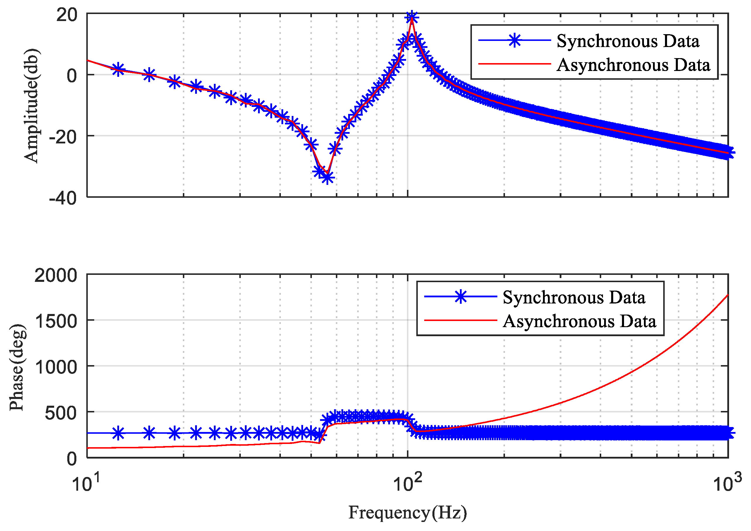
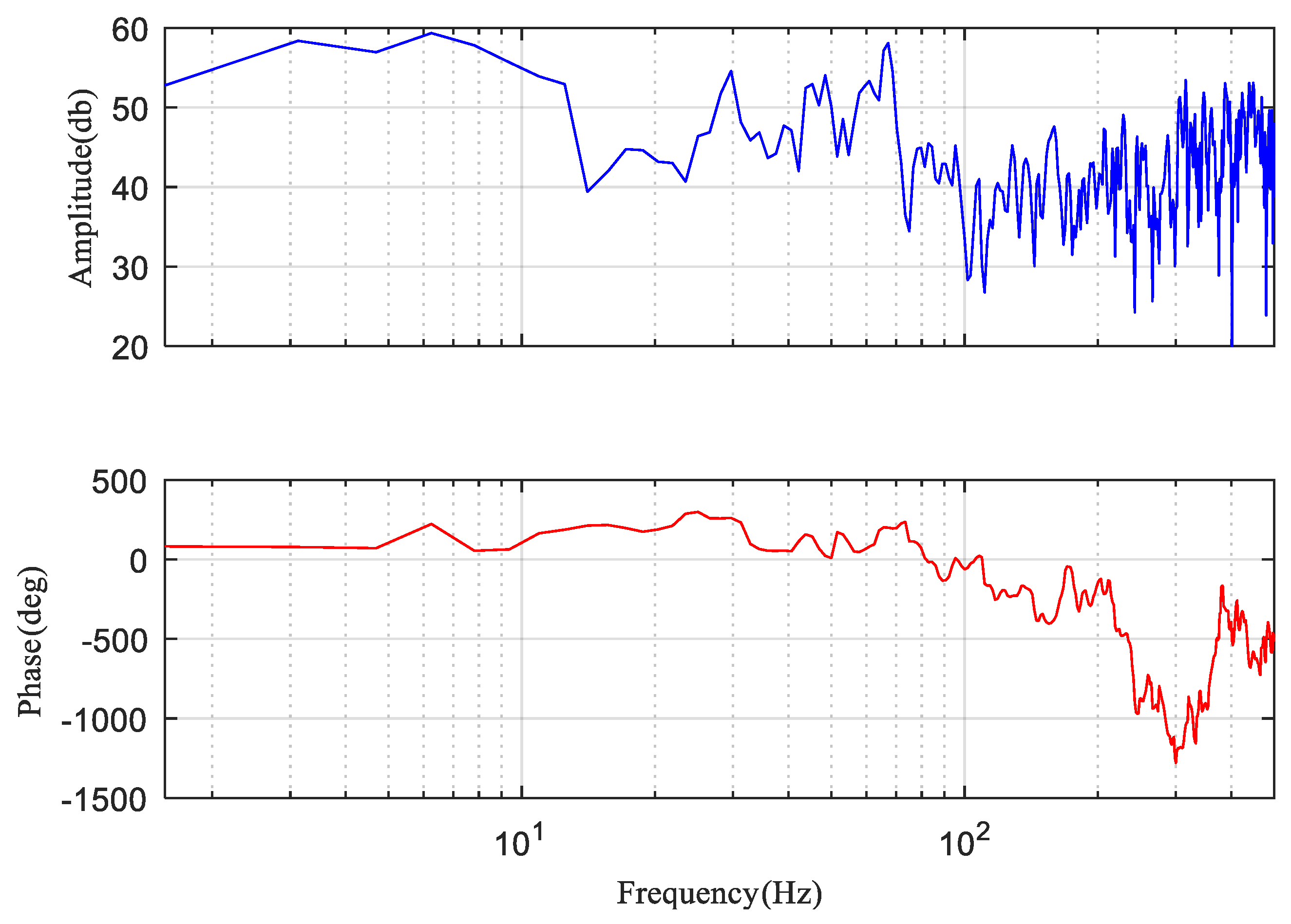
3.4. Calculation of the Frequency Response Function

Generally, the FRF of the system input signal $x(t)$ and output signal $y(t)$ is given by the ratio between the spectral density function $G_{xy}(\omega )$ and $G_{xx}(\omega )$ as follows:

$$H(\omega )=\frac{G_{xy}(\omega )}{G_{xx}(\omega )}=\left|H(\omega )\right|e^{j\varphi \left(\omega \right)}$$

(29)

where $H(\omega )$ is the FRF of the system, $G_{xy}(\omega )$ is the cross-power spectral density of the input $x(t)$ and output $y(t)$, and $G_{xx}(\omega )$ is the self-power spectral density of the input signal $x(t)$.

3.5. Levenberg-Marquardt Algorithm

Section 3.3 introduced the error criterion function, and this section uses the L-M algorithm to iterate on it to find the optimal value.

Error function:

$$E\left(x\right)={\displaystyle \sum _{k=1}^n{e}_k\left(x\right)}$$

(30)

For Newton’s law, the iterative formula is:

$$x^{k+1}=x^k+\Delta x$$

(31)

$$\Delta x=-{[{\nabla }^{2}E(x)]}^{-1}•\nabla E(x)$$

(32)

where $e_k\left(x\right)$ is the error, $n$ is the total number of points in the identification frequency domain window, and $x$ are the parameters to be identified. $x^k$ is the input vector at the k-th iteration, and $x^{k+1}$ is the input vector at the (k+1)-th iteration. $\nabla E(x)$ and ${\nabla }^{2}E(x)$ are the gradient and the Hessian matrix of the error criterion function $E(x)$ respectively.

$$\nabla E(x)=J^T(x)e(x)$$

(33)

$${\nabla }^{2}E(x)=J^T(x)J(x)+S(x)$$

(34)

In the above two formulas, $S(x)={\displaystyle \sum _{k=1}^n\left[e_k(x){\nabla }^2{e}_k(x)\right]}$, $J$ is the Jacobian matrix, namely:

$$J(x)=\left[\begin{array}{cccc}\frac{\partial e_1(x)}{\partial x_1}& \frac{\partial e_1(x)}{\partial x_2}& \dots & \frac{\partial e_1(x)}{\partial x_n}\\ \frac{\partial e_2(x)}{\partial x_1}& \frac{\partial e_2(x)}{\partial x_2}& \dots & \frac{\partial e_2(x)}{\partial x_n}\\ \dots & \dots & \dots & \dots \\ \frac{\partial e_n(x)}{\partial x_1}& \frac{\partial e_n(x)}{\partial x_2}& \dots & \frac{\partial e_n(x)}{\partial x_n}\end{array}\right]$$

(35)

The calculation method of the Gauss-Newton method is:

$$\Delta x={[J^T(x)J(x)]}^{-1}J(x)e(x)$$

(36)

The L-M algorithm is an improved form, namely:

$$\Delta x={[J^T(x)J(x)+\mu I]}^{-1}J(x)e(x)$$

(37)

where $I$ is the identity matrix. $\mu$ is the damping coefficient, and $\mu$ needs to be adjusted during each iteration: When $L$ decreases quickly, a smaller $\mu$ value is used. At this time, the method is similar to the Gauss–Newton method. When $L$ decreases slowly, the $\mu$ value is increased, and the method is similar to the gradient method [29].

Figure 4 shows the flowchart of the parameter identification process, which can be summarized as follows:

(1)

The dynamic model of a single robot joint is established.

(2)

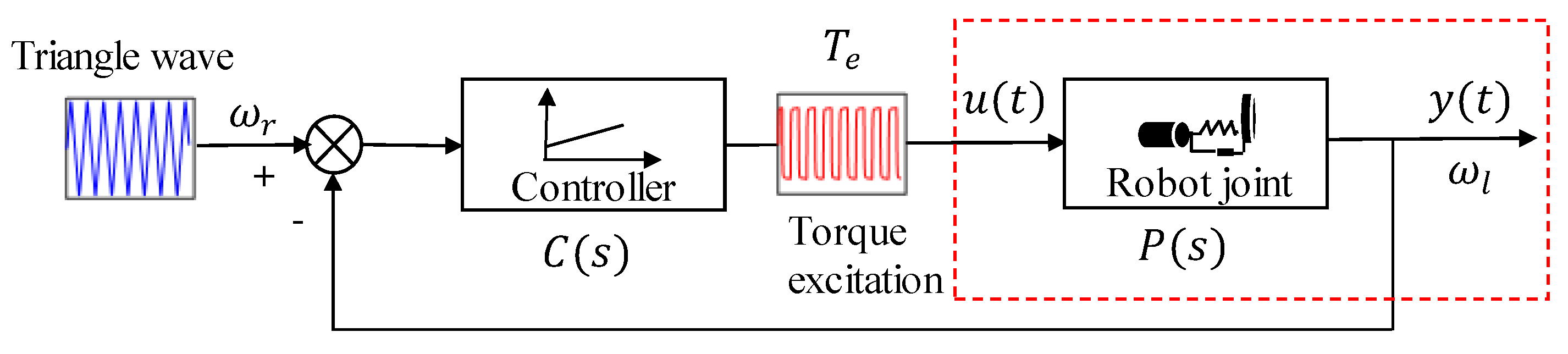
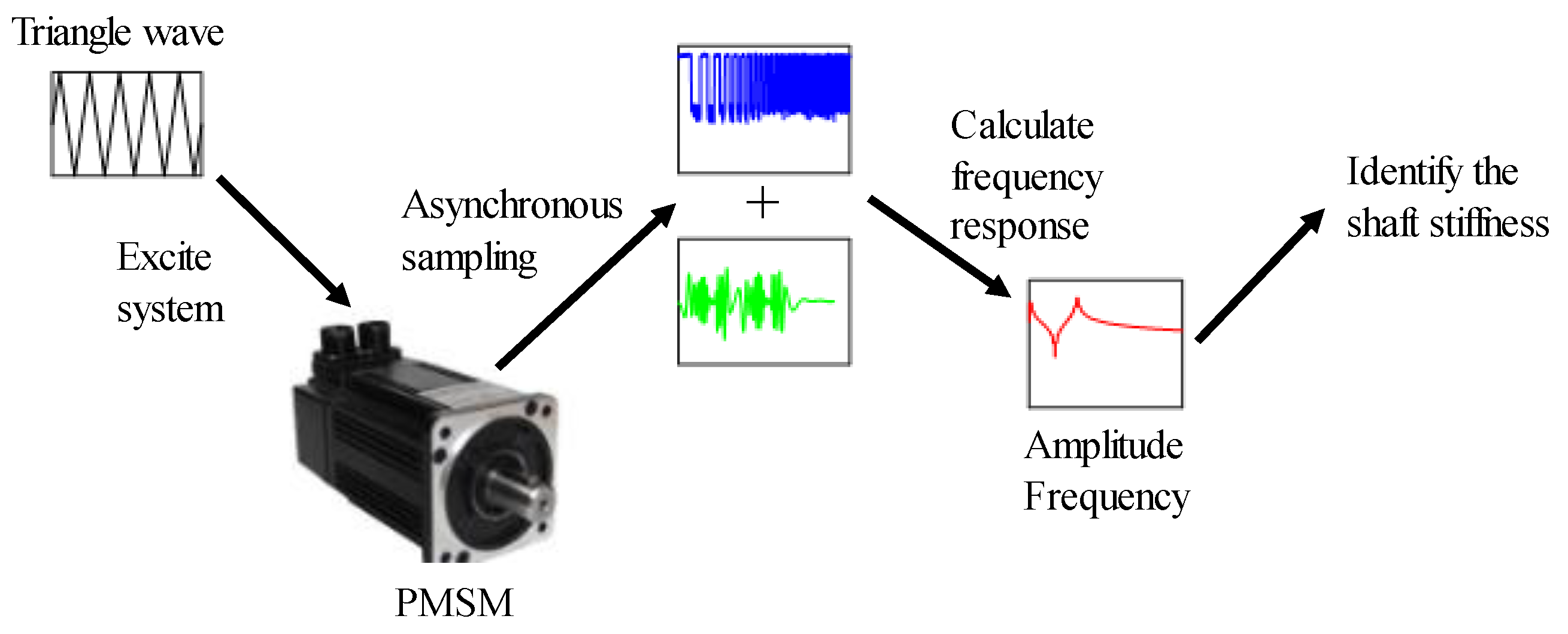
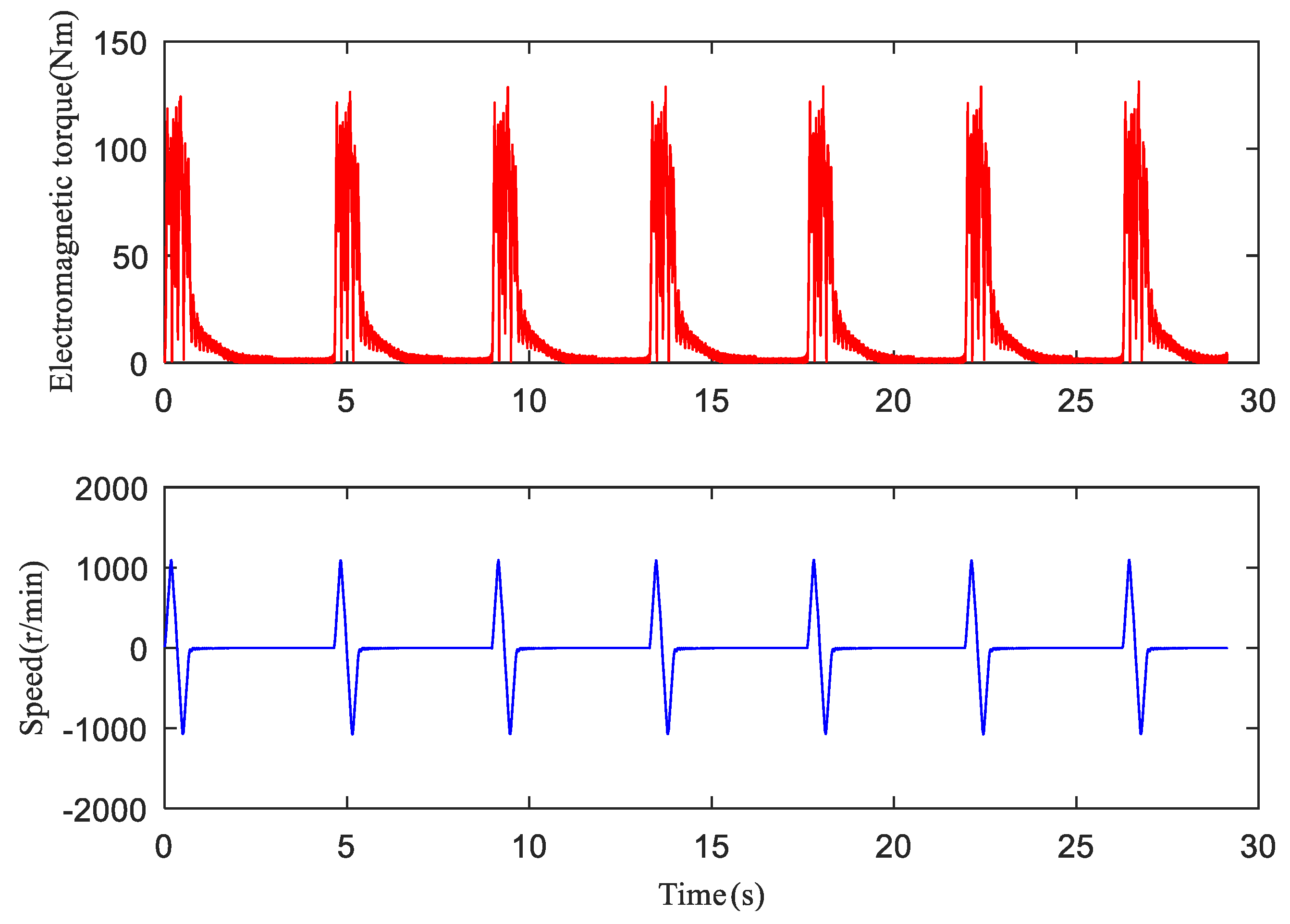
The speed command signal is set as a triangle wave so that the electromagnetic torque follows a rectangular window to excite the system.

(3)

The current signal and the motor encoder signal are collected to calculate the electromagnetic torque and the motor speed.

(4)

The ratio between the cross-power spectrum of input and output signals and the self-power spectrum of input signals is calculated to obtain the amplitude of the FRF.

(5)

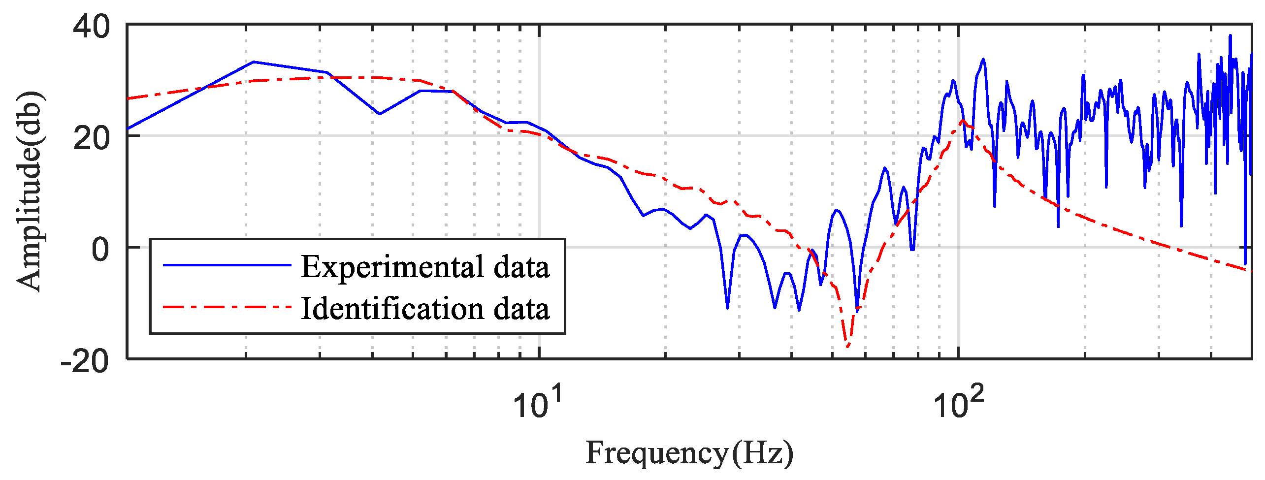
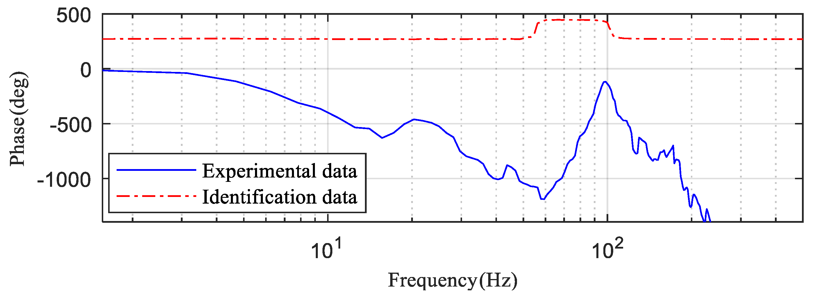
The L-M optimization algorithm is used to fit the experimental and theoretical amplitude of the FRF to minimize the error.

(6)

The shaft stiffness is identified from the amplitude of the FRF.

4. Simulations

According to the dynamic equations of the single joint degree of freedom system introduced in Section 1, a simulation model of the articulated arm motion was built. The parameters used in the simulation correspond to the actual parameters of the test bench, the structure of the test bench and its parameters are described in detail in Section 5.1. The joint stiffness is the equivalent stiffness of the coupling stiffness and the reducer stiffness in series, and the value is $891 N·m/\text{rad}$.The inertia of the motor side is the sum of the inertia of the motor and the inertia of the reducer, and the value is $0.003027 \text{kg}·m^2$. The equivalent inertia on the load side is $0.00748 \text{kg}·m^2$.

The speed command was set as a triangular wave to excite the system using rectangular wave electromagnetic torques. The top speed was 1000 r/min, and the movement period was 0.4 s, and the total simulation time was set to 2 s.

The amplitude of the FRF and the phase of the FRF of the system are performed using synchronous data and asynchronous data, respectively, as shown in the Figure 5. According to Equations (5) and (6), the theoretical resonance frequencies ARF and ATF of the system are calculated as ${\omega }_{ARF}=54.96$ Hz, ${\omega }_{NTF}=102.39$ Hz. The two frequencies are consistent with the resonance frequency obtained by the simulation model in Figure 5, which shows the accuracy of the simulation model. The amplitude frequency characteristics obtained by asynchronous data and synchronous data are the same. However, the asynchronous data has a phase shift.

Data in the range of 0–500 Hz in the FRF and the amplitude of the FRF, respectively, were used to identify the stiffness of the shaft system using the L-M optimization algorithm. Firstly, the conventional identification method based on the FRF was used to identify the synchronous data. In this case, the identification result is 866.13 $N·m/\text{rad}$ and the error is 2.79%, the identification accuracy is satisfactory. However, for asynchronous data, identification result of the identification method based on the FRF is 654.67 $N·m/\text{rad}$ and the error reaches 26.52%. The result is unacceptable, it shows that the FRF is not applicable for asynchronous data.

However, the identification method of the amplitude of the FRF obtains accurate results for asynchronous data. The stiffness identification result is 859.13 $N·m/\text{rad}$ and the error is 3.49%.

Table 1. Stiffness identification result of the synchronous and asynchronous data.

Data	True Value $(\mathrm{N}·\mathrm{m}/\text{rad})$	Identification Result $(\mathrm{N}·\mathrm{m}/\text{rad})$	Error (%)
FRF of the synchronous data	891	866.13	2.79
FRF of the asynchronous data	891	654.67	26.52
amplitude of FRF of the asynchronous data	891	859.93	3.49

shows the stiffness identification results of the three cases. It proves that the proposed method can avoid phase error, and it is feasible and comparable to applying the complete frequency response for identification.

5. Experimental Identification

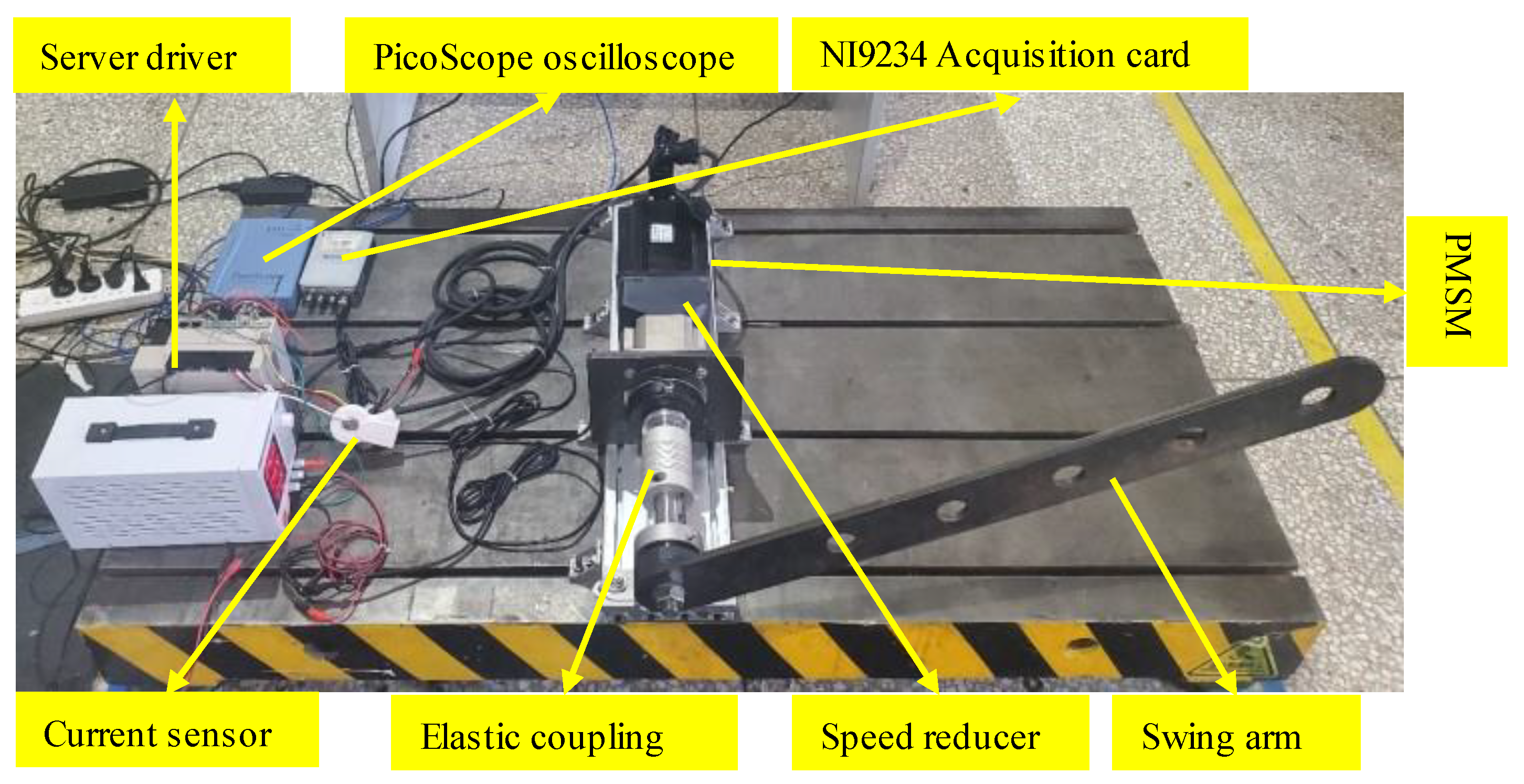
5.1. Experimental System

A single-degree-of-freedom articulated arm test bench was built to simulate the motion of an industrial robot single joint. The entire setup is shown in Figure 6. The transmission system comprises a speed reducer and a shaft. Moreover, the elastic coupling is connected in series with the shaft and the speed reducer. The PLC model is a SIEMENS 1212c connected to the driver to control the motor motion. An oscilloscope is used to obtain the encoder signal from the driver. The current sensor is placed on one of the power lines, and the NI9234 acquisition card is used to collect the line current data. The input and output data collected are asynchronous. The specific parameters of the test bench are listed in

Table 2. Parameters of the experimental system.

Parameter	Value
PMSM rated power	2.3 $\text{KW}$
PMSM torque constant	3 $N·m/A$
Moment of inertia of PMSM	$2.77\times {10}^{-3} \text{kg}·{\mathrm{m}}^2$
Moment of inertia of reducer	$2.57\times {10}^{-4} \text{kg}·{\mathrm{m}}^2$
Reduction ratio	$10:1$
Articulated arm mass	5 $\text{kg}$
Articulated arm length	75 $\text{cm}$
Moment of inertia of articulated arm	$0.748 \text{k}·{\text{m}}^2$
Reducer stiffness	$89595 N·m/\text{rad}$
Elastic coupling stiffness	$900 N·m/\text{rad}$

.

During the experiment, the triangular wave was set as the command speed to produce the electromagnetic torque as a rectangular wave to excite the system. Two motion conditions were set, and the acceleration time and deceleration time of the first group were both set to 0.5 s. Furthermore, the acceleration time and deceleration time of the second group were both set to 0.2 s. In these two conditions, the joint arm swings back and forth 120 degrees in each motion cycle.

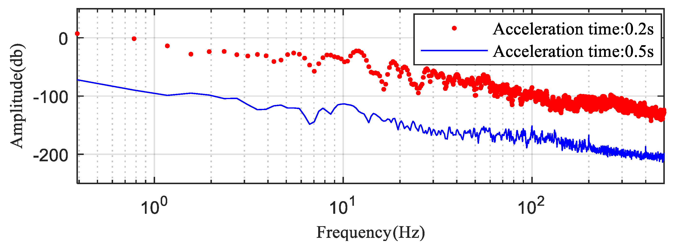
5.2. The Impact of the Acceleration Time on Excitation

The electromagnetic torque is obtained by multiplying the envelope of the current and the motor torque constant. The motor encoder signal is processed to obtain the motor speed. Because the current signal and the motor encoder signal are collected separately and have different sampling rates, it is necessary to resample the sampling rate of the two signals through interpolation so that they are consistent. Figure 7 shows the input signals and the output signals of the test bench for an acceleration time of 0.5 s. Figure 8 shows the frequency response of the system when the acceleration time is 0.5 s. No evident resonance peaks are found on the amplitude and phase of the FRF, indicating that the system is not sufficiently excited, and it is impossible to identify the parameters.

Then, the acceleration time is set to 0.2 s, and the torque and speed obtained are shown in Figure 9. The amplitude and the phase of the FRF of the system are obtained, as shown in Figure 10 and Figure 11. Evident resonance can be observed in the two Figures.

Figure 12 shows the power spectrum of the electromagnetic torque at 0.2 s and 0.5 s acceleration time. The power spectrum of the two types of electromagnetic torque has a wide enough frequency band. However, the intensity decreases with increasing frequency. At the position of resonance frequency, the intensity of the two types of excitation signals is not significant. The amplitude is approximately −170 dB when the acceleration time is 0.5 s, and the amplitude is approximately −100 dB when the acceleration time is 0.2 s. The success of the latter excites the system, indicating that the shorter the reciprocating time, the stronger the excitation signal, and the easier it is to excite the system.

5.3. Parameter Identification

The FRF and the amplitude of the FRF of the system with an acceleration time of 0.2 s were used for identification respectively, including the frequency range of 0–500 Hz. Because the torsional stiffness was our focus, we only identified stiffness first and considered that inertias were known. The identification results of the two methods are shown in

Table 3. Stiffness identification results of the FRF and the amplitude of FRF.

Data	True Value $(\mathrm{N}·\mathrm{m}/\text{rad})$	Identification Result $(\mathrm{N}·\mathrm{m}/\text{rad})$	Error (%)
FRF of the asynchronous data	891	1229	37.93
amplitude of FRF of the asynchronous data	891	851.9	4.49

. Since the data collected in the experiment are asynchronous, there is phase deviation in the FRF. Therefore, when the traditional identification method based on FRF is used, the identification error reaches 37.93%. The proposed identification method is based on the amplitude of the FRF, which avoids phase error and obtains accurate identification results. The identified value is $851.9 N·m/\text{rad}$, and the error is 4.49%.

The effectiveness of the method was tested for multiple unknowns. In this regard, the two inertia parameters were regarded as unknowns and identified along with torsional stiffness. The results are listed in

Table 4. Identification results of the three parameters.

Parameter	True Value	Initial Value	Initial Error (%)	Identification Result	Identification Error (%)
$K$($\mathrm{N}·\mathrm{m}/\text{rad}$)	891	100	88.78	807.34	9.39
$J_m$($\text{kg}·{\text{m}}^2$)	0.003027	0.001	66.96	0.00292	3.53
$J_l$($\text{kg}·{\text{m}}^2$)	0.00748	0.005	33.16	0.00676	9.57

. As seen in the table, the identification accuracy of torsional stiffness declines when the unknown parameters increase compared with that of the simulation; the error of the torsional stiffness reaches 9.39%. Thus, simultaneously identifying multiple parameters increases the calculation error. In contrast, the identification errors of the three parameters are all below 10%, indicating that not only the stiffness can be identified. However, motor inertia and load inertia can also be identified.

Figure 10 shows the spectrum of the amplitude of the FRF generated by the experimental and identified data. As seen in the Figure, the identified resonance frequencies agree well with the experimental resonance frequencies when only the locations of the anti-resonance and resonance frequencies are considered. However, note that a certain difference exists between the identified amplitude and the experimental amplitude. The reason is the damping effect that is neglected in the identification, and there is noise interference in the experiment.

Figure 11 shows the spectrum of the phase of the FRF generated by the experimental and identified data. When the input and output data of the experiment are asynchronous, although the resonance frequency can be identified, the phase of the FRF of the experimental data and the identification data have a substantial deviation. Therefore, the phase of the FRF leads to identification errors when the input and output data are asynchronous. Nevertheless, the identification method of the amplitude of the FRF avoids the phase error, which can replace the identification method based on the FRF.

6. Conclusions

In this study, aiming at identifying the torsional stiffness of industrial robot joints, we proposed an operational identification method. The novelty of this method relies on using motion excitation to excite the system and the amplitude of the FRF for parameter identification. The proposed method can function without affecting the normal working state of the robot. The experiments and simulations showed the effectiveness of the proposed method. More importantly, the stiffness, motor inertia, and load inertia could be identified. The future work will focus on further enriching the identifiable parameters, including the identification of electrical parameters.

References

1. Madsen, E.; Rosenlund, O.S.; Brandt, D. Comprehensive modeling and identification of nonlinear joint dynamics for collaborative industrial robot manipulators. Control Eng. Pract. 2020, 101, 104462. [Google Scholar] [CrossRef]
2. Morales-Velazquez, L.; Romero-Troncoso, R.; Osornio-Rios, R.A.; Herrera-Ruiz, G.; de Santiago-Perez, J.J. Special purpose processor for parameter identification of CNC second order servo systems on a low-cost FPGA platform. Mechatronics 2010, 20, 265–272. [Google Scholar] [CrossRef]
3. Choi, S.; Seong, M.; Ha, S. Accurate position control of a flexible arm using a piezoactuator associated with a hysteresis compensator. Smart Mater. Struct. 2013, 22, 045009. [Google Scholar] [CrossRef]
4. Shitole, C.; Sumathi, P. Sliding DFT-based vibration mode estimator for single-link flexible manipulator. IEEE/ASME Trans. Mechatron. 2015, 20, 3249–3256. [Google Scholar] [CrossRef]
5. Meng, D.; She, Y.; Xu, W. Dynamic modeling and vibration characteristics analysis of flexible-link and flexible-joint space manipulator. Multibody Syst. Dyn. 2018, 43, 321–347. [Google Scholar] [CrossRef]
6. Dwivedy, S.K.; Eberhard, P. Dynamic analysis of flexible manipulators, a literature review. Mech. Mach. Theory 2006, 41, 749–777. [Google Scholar] [CrossRef]
7. Xu, J.; Zhu, J.; Wan, L. Effects of intermediate support stiffness on nonlinear dynamic response of transmission system. J. Vib. Control 2020, 26, 851–862. [Google Scholar] [CrossRef]
8. Toliyat, H.A.; Levi, E.; Raina, M. A review of RFO induction motor parameter estimation techniques. IEEE Trans. Energy Convers. 2003, 18, 271–283. [Google Scholar] [CrossRef]
9. Chunyu, Y.; Lingchao, B.; Bin, C. Energy modeling and online parameter identification for permanent magnet synchronous motor driven belt conveyors. Measurement 2021, 178, 109342. [Google Scholar]
10. Underwood, S.J.; Husain, I. Online parameter estimation and adaptive control of permanent-magnet synchronous machines. IEEE Trans. Ind. Electron. 2010, 57, 2435–2443. [Google Scholar] [CrossRef]
11. Xiao, X.; Chen, C.; Zhang, M. dynamic permanent magnet flux estimation of permanent magnet synchronous machines. IEEE Trans. Appl. Supercond. 2010, 20, 1085–1088. [Google Scholar] [CrossRef]
12. Beineke, S.; Schutte, F.; Wertz, H. Comparison of parameter identification schemes for self-commissioning drive control of nonlinear two-mass systems. In Proceedings of the IEEE Industry Applications Conference, New Orleans, LA, USA, 5–9 October 1990; pp. 493–500. [Google Scholar]
13. Villwock, S.; Pacas, M. Application of the welch-method for the identification of two- and three-mass-systems. IEEE Trans. Ind. Electron. 2008, 55, 457–466. [Google Scholar] [CrossRef]
14. Pacas, M.; Villwock, S.; Szczupak, P. Methods for commissioning and identification in drives. COMPEL Int. J. Comput. Math. Electr. Electron. Eng. 2010, 29, 53–71. [Google Scholar] [CrossRef]
15. Zoubek, H.; Pacas, M. Encoderless identification of two-mass-systems utilizing an extended speed adaptive observer structure. IEEE Trans. Ind. Electron. 2017, 64, 595–604. [Google Scholar] [CrossRef]
16. Zha, F.; Sheng, W.; Guo, W.; Qiu, S.; Deng, J.; Wang, X. Dynamic parameter identification of a lower extremity exoskeleton using RLS-PSO. Appl. Sci. 2019, 9, 324. [Google Scholar] [CrossRef] [Green Version]
17. Ostring, M.; Gunnarsson, S.; Norrloef, M. Closed-loop identification of an industrial robot containing flexibilities. Control Eng. Pract. 2003, 11, 291–300. [Google Scholar] [CrossRef]
18. Urrea, C.; Pascal, J. Design, simulation, comparison and evaluation of parameter identification methods for an industrial robot. Comput. Electr. Eng. 2016, 67, 791–806. [Google Scholar] [CrossRef]
19. Bazanellaa, S.; Gevers, M.; Miskovic, L. Closed-loop identification of MIMO systems: A new look at identifiability and experiment design. Eur. J. Control 2007, 16, 228–239. [Google Scholar] [CrossRef] [Green Version]
20. Zoubek H and Pacas, M. A method for speed-sensorless identification of two-mass-systems. In Proceedings of the IEEE Energy Conversion Congress and Exposition, Atlanta, GA, USA, 12–16 September 2010; pp. 4461–4468. [Google Scholar]
21. Nevaranta, N.A.; Derammelaere, S.B.; Parkkinen, J.A. Online identification of a two-mass system in frequency domain using a Kalman filter. Modeling Identif. Control 2016, 37, 133–147. [Google Scholar] [CrossRef] [Green Version]
22. Fang, Y.; Hu, J.; Liu, W. Smooth and time-optimal S-curve trajectory planning for automated robots and machines. Mech. Mach. Theory 2019, 137, 127–153. [Google Scholar] [CrossRef]
23. Mesloub, H.; Boumaaraf, R.; Benchouia, M.T. Comparative study of conventional DTC and DTC_SVM based control of PMSM motor-Simulation and experimental results. Math. Comput. Simul. 2020, 167, 296–307. [Google Scholar] [CrossRef]
24. Chou, H.-H.; Kung, Y.-S.; Quynh, N.V.; Cheng, S. Optimized FPGA design, verification and implementation of a neuro-fuzzy controller for PMSM drives. Math. Comput. Simul. 2013, 90, 28–44. [Google Scholar] [CrossRef]
25. Azzoug, Y.; Sahraoui, M.; Pusca, R.; Ameid, T.; Romary, R.; Cardoso, A.J.M. High-performance vector control without AC phase current sensors for induction motor drives: Simulation and real-time implementation. ISA Trans. 2021, 109, 295–306. [Google Scholar] [CrossRef]
26. Zhang, Q.; Tan, L.; Xu, G. Evaluating transient performance of servo mechanisms by analysing stator current of PMSM. Mech. Syst. Signal Process. 2018, 101, 535–548. [Google Scholar] [CrossRef]
27. Brancati, R.; Rocca, E.; Lauria, D. Feasibility study of the Hilbert transform in detecting the gear rattle phenomenon of automotive transmissions. J. Vib. Control 2018, 24, 2631–2641. [Google Scholar] [CrossRef]
28. Montonen, J.H.; Nevaranta, N.; Lindh, T.; Alho, J.; Immonen, P.; Pyrhönen, O. Experimental identification and parameter estimation of the mechanical driveline of a hybrid bus. IEEE Trans. Ind. Electron. 2017, 65, 5921–5930. [Google Scholar] [CrossRef]
29. Cárdenas-Garcia, J.F.; Ekwaro-Osire, S.; Berg, J.M. Non-linear Least-squares Solution to the Moiré Hole Method Problem in Orthotropic Materials. Part I: Residual Stresses. Exp. Mech. 2005, 45, 301–313. [Google Scholar] [CrossRef]
Figure 1. The schematic diagram of a single joint of an industrial robot.
Machines 09 00204 g001
Figure 2. Dual-mass models of the robot joint.
Machines 09 00204 g002
Figure 3. Block diagram of closed loop speed control of robot.
Machines 09 00204 g003
Figure 4. Identification method flowchart.
Machines 09 00204 g004
Figure 5. Spectrum of the frequency response in simulation.
Machines 09 00204 g005
Figure 6. Single degree of freedom articulated arm test bench.
Machines 09 00204 g006
Figure 7. Input and output signal of the test bench when the acceleration time was 0.5 s.
Machines 09 00204 g007
Figure 8. Frequency response of the test bench with acceleration time of 0.5 s.
Machines 09 00204 g008
Figure 9. Input and output signal of the test bench when the acceleration time was 0.2 s.
Machines 09 00204 g009
Figure 10. Amplitude of the FRF of experimental and identified data.
Machines 09 00204 g010
Figure 11. Phase of the FRF of experimental and identified data.
Machines 09 00204 g011
Figure 12. Power spectrum of the electromagnetic torque.
Machines 09 00204 g012