A Unified Framework for the H_∞ Mixed-Sensitivity Design of Fixed Structure Controllers through Putinar Positivstellensatz  ^†

Abstract

In this paper, we present a novel technique to design fixed structure controllers, for both continuous-time and discrete-time systems, through an $H_{\infty }$ mixed sensitivity approach. We first define the feasible controller parameter set, which is the set of the controller parameters that guarantee robust stability of the closed-loop system and the achievement of the nominal performance requirements. Then, thanks to Putinar positivstellensatz, we compute a convex relaxation of the original feasible controller parameter set and we formulate the original $H_{\infty }$ controller design problem as the non-emptiness test of a set defined by sum-of-squares polynomials. Two numerical simulations and one experimental example show the effectiveness of the proposed approach.

1. Introduction

The development of a worst-case control design for a linear plant subjected to unknown parameter uncertainties and disturbances has attracted the interest of the control community for many years. In [1], within the context of sensitivity reduction, Zames introduces the $H_{\infty }$ norm minimization to formulate the control design problem. The mixed-sensitivity approach, introduced in [2,3], is a general control design formulation where the $H_{\infty }$ norm is used to define constraints on both the sensitivity and complementary sensitivity function. These constraints are defined by suitable weighting functions to ensure good performances and the robustness of the system to be controlled. The books [4,5] and the paper [6] provide a deep discussion about the underlying theory and, starting from robustness and time-domain requirements, the way to suitably formulate the mixed-sensitivity control design problem.

Nominal $H_{\infty }$ mixed-sensitivity control design problem can be solved through algorithms based on linear matrix inequalities (LMI) (see, e.g., [7,8]) or on the algebraic Riccati equation (see, e.g., [9,10]). Most of the $H_{\infty }$ mixed-sensitivity control design approaches are developed for continuous-time systems, while a few approaches deal with the discrete-time systems. In [11,12], discrete-time controllers are designed through the solution of two Riccati equations, while a convex optimization approach is proposed in [13]. The interested reader is referred to [14], and references therein, for a deeper discussion on discrete-time $H_{\infty }$ mixed-sensitivity control design.

In general, algorithms for $H_{\infty }$ control synthesis cannot take into account the order of the controller, which instead depends on the order of the transfer functions defining the underlying optimization problem. However, in several practical applications, like PI and PID controllers or embedded control systems, the controller structure is a-priori fixed and cannot be modified. In [15], the authors show that controller structure constraints make the $H_{\infty }$ control design problem non-convex and NP-hard to be solved. The main difficulty is that structural constraints produce bilinear matrix inequalities (BMI) [16], that are non-convex. Convexification methods to transform the BMIs constraints in LMIs through variable change (see, e.g., [17]) or inner convex approximations (see, e.g., [18]) are proposed in the literature. However, the success of these methods depends on the specific structure of the constraints and cannot be generalized. A common approach to BMIs problems is represented by iterative algorithms (see, e.g., [19,20,21,22] and references therein) that finds local optimum solutions in polynomial time.

To avoid numerical difficulties related to BMIs, some techniques based on the controller or the plant order reduction have been proposed in [23,24,25]. However, the plant order reduction leads to higher conservatism in the uncertainty model, while the controller order reduction leads to performances degradation. Moreover, these techniques still cannot ensure a specific controller structure (e.g., PID).

Burke et al., in [26], propose a gradient sampling algorithm for the design of a fixed-order $H_{\infty }$ controller, which is implemented in the HIFOO Matlab toolbox (see [27]). Another Matlab toolbox for the design of fixed-structure controllers is Hinfstruct, which implements the algorithm proposed in [28] and is based on the Clarke sub-differential approach presented in [29]. Both these Matlab packages are based on local optimization techniques, which have no guarantees about the convergence to the global optimal solution.

A few approaches based on global optimization have also been proposed in the literature to design fixed structure controllers. These approaches require a parametric representation of uncertain plants and exploit interval arithmetic tools to synthesize the $H_{\infty }$ control problem. In [30], the authors present a remarkable result by providing a branch-and-bound based algorithm to compute inner and outer approximations of the controller parameter set. Other global optimization-based approaches rely on quantifier elimination techniques (see, e.g., [31]).

Among the several structures, the $H_{\infty }$ mixed-sensitivity design of PID controllers is the most investigated in the literature. Convex optimization techniques have been proposed in [32,33] to tune continuous-time PID controllers, while bilinear transformation is used to compute discrete-time regulators in [34]. The main difficulty related to the fixed-structure controller design is related to the non-convexity of the stabilizing parameter set. For linear parametrized controllers, inner convex approximations are proposed in [35,36,37].

In this paper, we propose a unified framework to design continuous and discrete-time fixed structure controllers in the framework of the mixed-sensitivity approach. Starting from the work [38], we extend the previous results to the most general case by considering both continuous and discrete-time systems. In the proposed algorithm, we first define the set of controller parameters that achieve robust stability and nominal performances of the feedback control system. Then, we rewrite the controller design problem as the positivity test over a bounded domain. By exploiting Putinar positivstellensatz theorem [39], we formulate the $H_{\infty }$ mixed sensitivity controller design as the non-emptiness test of a convex set defined through a number of sum of squares (SOS) polynomial constraints. The problem to be solved is a convex semi-definite problem (SDP), whose solution can be found in polynomial time.

The paper is organized as follows: Section 2 reviews $H_{\infty }$ mixed-sensitivity notations and backgrounds fundamentals, while the problem formulation is given in Section 3. In Section 4, we present the proposed $H_{\infty }$ control design approach based on the Putinar positivstellensatz. Numeric examples are provided in Section 5, to show the effectiveness of the proposed methods to design both continuous and discrete-time controllers, together with the results obtained with the Matlab function Hinfstruct. Section 6 shows experimental results of the controller design problem for a magnetic suspension system, and Section 7 concludes the paper.

2. Notations and Background

In this section, we introduce the notations that are used in the paper and review some basics on $H_{\infty }$ mixed sensitivity controller design. We define the transfer functions through a generic variable $\xi \in \mathbb{C}$ which is $\xi =s$ when dealing with continuous time (CT) systems and $\xi =z$ for discrete time (DT) systems. Given a transfer function $C\left(\xi \right)$, we denote with $C\left(j\omega \right)$ the frequency response computed by assigning $\xi =j\omega$ for CT systems and $\xi =e^{j\omega T_s}$ for DT systems, where $T_s$ is the sampling time.

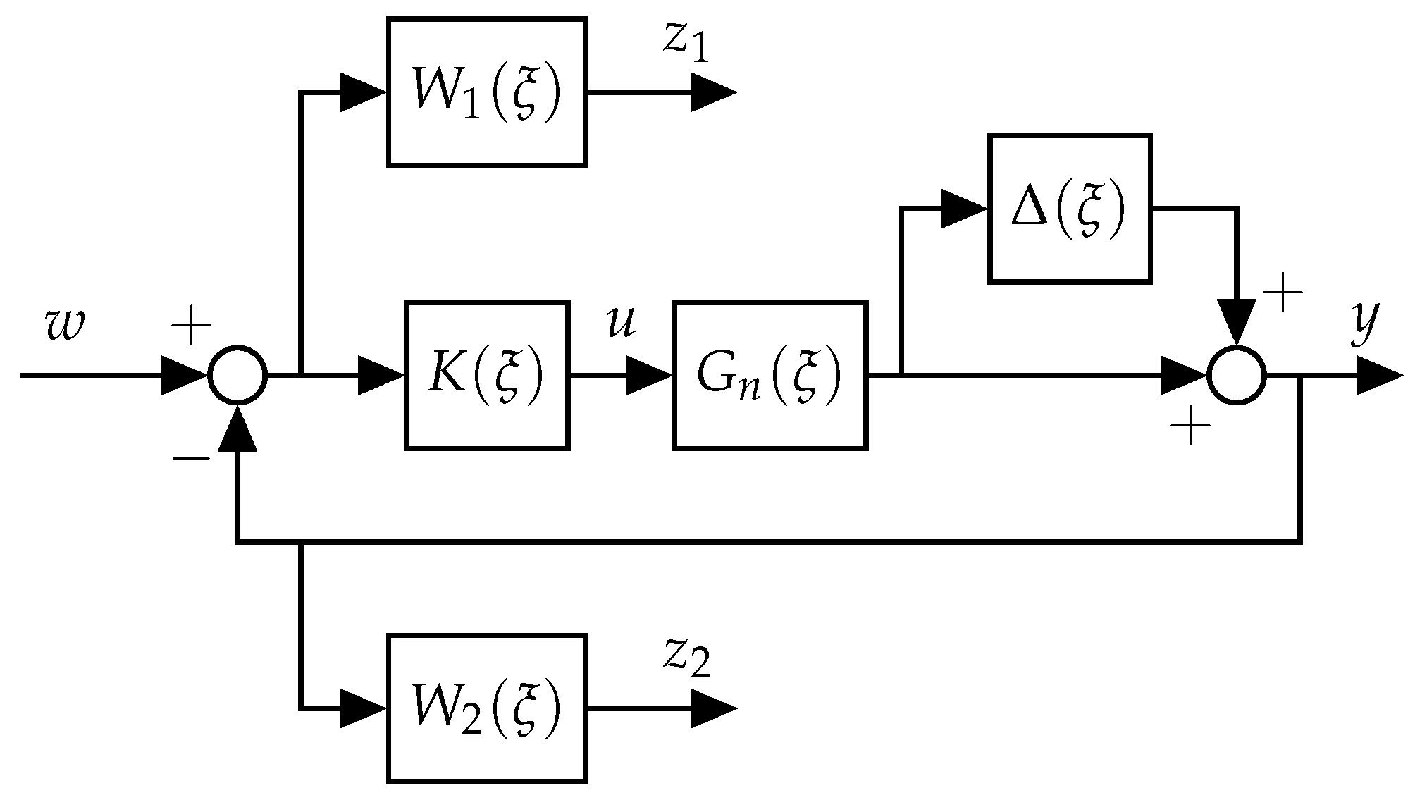
Let us consider the feedback control system depicted in Figure 1, where $G_n\left(\xi \right)$ and $K\left(\xi \right)$ are the nominal plant and the controller transfer functions, respectively, $w\in \mathbb{R}$ is the reference signal, $u\in \mathbb{R}$ is the control input, $y\in \mathbb{R}$ is the measured output and $z_1\in {\mathbb{R}}^{n_1}$ and $z_2\in {\mathbb{R}}^{n_2}$ are the controlled outputs associated to the assigned performance requirements.

Figure 1. Block diagram of feedback system.

Let $G\left(\xi \right)$ be the uncertain model of the plant described by

$$G\left(\xi \right)=G_n\left(\xi \right)(1+\Delta \left(\xi \right))$$

(1)

where $\Delta \left(\xi \right)\in \mathbb{C}$ is unstructured multiplicative uncertainty, which is bounded by a given transfer function $W_u\left(\xi \right)$, i.e.,

$$|\Delta \left(\xi \right)|\le |W_u\left(\xi \right)|,\forall \omega \in \Omega$$

(2)

such that $\Omega =[0,+\infty )$ for CT systems and $\Omega =\left[0,\frac{\pi }{T_s}\right]$ for DT systems.

$W_1\left(\xi \right)$ and $W_2\left(\xi \right)$ are suitable weighting functions that describe the performance constraints on the nominal sensitivity $S_n\left(\xi \right)$ and nominal complementary sensitivity transfer function $T_n\left(\xi \right)$, respectively. For a given nominal plant $G_n\left(\xi \right)$ and a controller $K\left(\xi \right)$, the nominal loop transfer function is defined as

$$L_n\left(\xi \right)=K\left(\xi \right)G_n\left(\xi \right),$$

(3)

the nominal sensitivity function and complementary sensitivity function are defined as

$$S_n\left(\xi \right)={(1+L_n\left(\xi \right))}^{-1}$$

(4)

and

$$T_n\left(\xi \right)=L_n\left(\xi \right){(1+L_n\left(\xi \right))}^{-1}$$

(5)

respectively. Nominal closed loop system performances constraints are met if

$$\begin{array}{cc}\hfill & \parallel S_n\left(\xi \right)W_1{\left(\xi \right)\parallel }_{\infty }\le 1\hfill \\ \hfill & \parallel T_n\left(\xi \right)W_2{\left(\xi \right)\parallel }_{\infty }\le 1\hfill \end{array}$$

(6)

where ${\parallel ·\parallel }_{\infty }$ is the $H_{\infty }$ norm of a dynamical system, which, for a generic single-input single-output (SISO) system $H\left(\xi \right)$, is

$${\parallel H\left(\xi \right)\parallel }_{\infty }=\underset{\omega \in \Omega }{sup}\left|H\left(j\omega \right)\right|.$$

(7)

In the remainder of this section, we review some definitions and results about feedback systems properties.

Definition 1.

A feedback system is said to be well-posed if all closed-loop transfer functions, defined from any exogenous input to all internal signals, are well-defined and proper.

Result 1.

A necessary and sufficient condition for well-posedness is that $S_n\left(\xi \right)$ exists and is proper, i.e., $1+K\left(\xi \right)G_n\left(\xi \right)$ is not strictly proper. A stronger condition for well-posedness is that either $K\left(\xi \right)$ or $G_n\left(\xi \right)$ be strictly proper transfer functions (see, e.g., [4]).

Definition 2.

A well-posed feedback system is internally stable if, and only if, all the transfer functions from any input to any output are BIBO stable (see, e.g., [40]).

Result 2.

Necessary and sufficient conditions for the internal stability of feedback systems are that (i) the nominal sensitivity function $S_n\left(\xi \right)$ is BIBO stable and (ii) there are no unstable zero/pole cancellations while forming the nominal loop function $L_n\left(\xi \right)$. [40] provides a detailed proof.

Definition 3.

A feedback system is robustly stable if the controller $K\left(\xi \right)$ makes the system internally stable for all possible uncertain plants.

Result 3.

By applying the small gain theorem (see, e.g., [40]), the system depicted in Figure 1 is robustly stable if the nominal sensitivity function $S_n\left(\xi \right)$ is stable and

$$\parallel T_n\left(\xi \right)W_u{\left(\xi \right)\parallel }_{\infty }\le 1$$

(8)

Further details can be found in [4].

3. Problem Formulation

In this section, we formulate the $H_{\infty }$ controller design problem for both CT and DT systems. In this work, we propose a methodology to design a $H_{\infty }$ controller $K(\xi ,\mathit{p})$ which guarantees robust stability to unstructured multiplicative uncertainty bounded by the function $W_u\left(\xi \right)$, and fulfils the nominal performance defined through the weighting functions $W_1\left(\xi \right)$ and $W_2\left(\xi \right)$. The controller is assumed to have a fixed structure, i.e., to belong to a certain class $\mathcal{K}$, which guarantees the well-posedness condition, and is characterized by an $n_k$-th order transfer function

$$K(\xi ,\mathit{p})=\frac{{\sum }_{i=0}^{n_k}{\beta }_i\left(\mathit{p}\right){\xi }^i}{{\xi }^{n_k}+{\sum }_{j=0}^{n_k-1}{\alpha }_j\left(\mathit{p}\right){\xi }^j}=\frac{N_k(\xi ,\mathit{p})}{D_k(\xi ,\mathit{p})}$$

(9)

where the denominator and numerator coefficients, ${\alpha }_j\left(\mathit{p}\right)\in \mathbb{R}$ and ${\beta }_i\left(\mathit{p}\right)\in \mathbb{R}$, are polynomial functions in a suitable parameter vector $\mathit{p}\in {\mathbb{R}}^{n_p}$ to be designed.

We assume to know the transfer functions $W_1\left(\zeta \right)$, $W_2\left(\zeta \right)$ and $W_u\left(\zeta \right)$, which take into account the design constraints, as well as the nominal plant transfer function defined as

$$G_n=\frac{N_g\left(\zeta \right)}{D_g\left(\zeta \right)}$$

(10)

where $N_g\left(\zeta \right)$ and $D_g\left(\zeta \right)$ are polynomial functions and $N_g\left(\zeta \right)$ has no roots at $s=0$ or $z=1$.

Remark 1.

It is worth noting that, since $K(\xi ,\mathit{p})$ depends on $\mathit{p}$, functions (3)–(5) involving K depend on the parameter vector $\mathit{p}$ as well. However, for the sake of simplicity, we omit $\mathit{p}$ as a parameter in all functions except for $K(\xi ,\mathit{p})$.

Definition 4.

We define the stabilizing controller parameter set

$$\mathcal{S}=\left\{\mathit{p}\in {\mathbb{R}}^{n_p}|K(\zeta ,\mathit{p})\mathit{internally}\mathit{stabilizes}{G}_n\left(\zeta \right)\right\}$$

(11)

as the set of all the controller parameters which guarantees the internal stability of the feedback control system depicted in Figure 1.

Definition 5.

By applying Result 3, we define the robust stabilizing controller parameter set

$${\mathcal{D}}_S=\left\{\mathit{p}\in \mathcal{S}|\parallel T_n\left(\xi \right)W_u{\left(\xi \right)\parallel }_{\infty }\le 1\right\}$$

(12)

as the set of all the controller parameters which guarantees the internal robust stability of the uncertain plant $G\left(\xi \right)$.

We can derive some properties of the selected controller class $\mathcal{K}$ through the analysis of the sets $\mathcal{S}$ and ${\mathcal{D}}_S$.

Result 4.

If the set $\mathcal{S}$ is empty then the chosen controller structure $\mathcal{K}$ is not suitable to provide stability of the nominal plant $G_n\left(\xi \right)$.

Result 5.

If the set ${\mathcal{D}}_s$ is empty then the chosen controller structure $\mathcal{K}$ is not suitable to provide robust stability of the uncertain plant $G\left(\xi \right)$.

Definition 6.

We define the feasible controller parameter set $\mathcal{D}$

$$\begin{array}{cc}\hfill \mathcal{D}=\left\{\mathit{p}\in {\mathcal{D}}_S|\right.& \parallel S_n\left(\xi \right)W_1{\left(\xi \right)\parallel }_{\infty }\le 1,\hfill \\ \hfill & \left.\parallel T_n\left(\xi \right)W_2{\left(\xi \right)\parallel }_{\infty }\le 1\right\}\hfill \end{array}$$

(13)

as the set of parameter $\mathit{p}$ which guarantee robust stability for the plant $G\left(\xi \right)$ and the achievement of the nominal performances described by the given weighting functions $W_1\left(\xi \right)$ and $W_2\left(\xi \right)$.

It is worth noting that, by considering Equations (6) and (13), the set $\mathcal{D}$ can be written equivalently as

$$\begin{array}{cc}\hfill \mathcal{D}=\left\{\mathit{p}\in \mathcal{S}|\right.& \parallel S_n\left(\xi \right)W_1{\left(\xi \right)\parallel }_{\infty }\le 1,\hfill \\ \hfill & \{\parallel T_n\left(\xi \right){\widehat{W}}_2{\left(\xi \right)\parallel }_{\infty }\le 1\}\hfill \end{array}$$

(14)

where ${\widehat{W}}_2\left(\xi \right)$ is such that

$$|{\widehat{W}}_2\left(j\omega \right)|=max\left\{|W_2\left(j\omega \right)|,|W_u\left(j\omega \right)|\right\},\forall \omega \in \Omega .$$

(15)

The emptiness of the set $\mathcal{D}$ highlights that the chosen controller class structure $\mathcal{K}$ is not suitable to achieve the closed-loop stability and desired closed-loop performance specifications. Instead, a large or unbounded set $\mathcal{D}$ may suggest that the controller structure may fulfil more demanding specifications.

Remark 2.

Through the procedure described in the next Section, it is possible to test several controller structures, e.g., a commercial solution, and to select the cheapest solution that guarantees the non-emptiness of the feasible controller parameters set.

4. An SOS Approach to Mixed Sensitivity Design with Fixed Structure Controller

In this section, we consider the problem of looking for a parameter vector $\mathit{p}$ belonging to the feasible controller parameters set $\mathcal{D}$. We rewrite this problem as the positivity check of a number of multivariate polynomials over a bounded semi-algebraic set. This problem, which is known to be NP-hard, can be efficiently solved by applying the Putinar positivstellensatz (see, e.g., [39] for details), through which the polynomial positivity check is reformulated in terms of SDP.

We rewrite $\mathcal{D}$ as the intersection of two sets $\mathcal{D}=\mathcal{S}\cap \mathcal{P}$, where the performance controller parameters set $\mathcal{P}$ is defined as

$$\begin{array}{cc}\hfill \mathcal{P}=\left\{\mathit{p}\in {\mathbb{R}}^{n_p}|\right.& \parallel S_n\left(\xi \right)W_1{\left(\xi \right)\parallel }_{\infty }\le 1,\hfill \\ \hfill & \{\parallel T_n\left(\xi \right){\widehat{W}}_2{\left(\xi \right)\parallel }_{\infty }\le 1\}\hfill \end{array}$$

(16)

The properties of the set $\mathcal{D}$ can be obtained through the analysis of the sets $\mathcal{S}$ and $\mathcal{P}$.

4.1. Mathematical Description of the Set $\mathcal{S}$

At first, we look for an explicit mathematical formulation of the set $\mathcal{S}$. For internal stability, both conditions of Result 2 must be satisfied. The first condition requires that the nominal sensitivity function $S_n\left(\xi \right)$ is stable, which is achieved if the roots of $1+L_n\left(\xi \right)$ have negative real part when dealing with CT systems, or have the module less than one when DT systems are considered.

4.1.1. Routh’s Stability Criterion

For CT systems, we can evaluate the sign of the real part of the roots of a polynomial function

$$A\left(s\right)=a_n{s}^n+a_{n-1}{s}^{n-1}+\dots +a_{1}s+a_0$$

(17)

by applying the Routh’s stability criterion, which is based on the Routh’s Table reported in Table 1 (further details on Routh’s stability criterion can be found in book [41]).

Table 1. Routh’s coefficients table.

${\mathit{a}}_{\mathit{n}}$	${\mathit{a}}_{\mathit{n}-2}$	${\mathit{a}}_{\mathit{n}-4}$	⋯
$a_{n-1}$	$a_{n-3}$	$a_{n-5}$	⋯
$b_1$	$b_2$	$b_3$	⋯
$c_1$	$c_2$	$c_3$	⋯
$d_1$	$d_2$	$d_3$	⋯
⋮	⋮	⋮	⋱

Coefficients $b_i$ in the Routh’s Table are given by

$$\begin{array}{cc}\hfill b_1=& \frac{a_{n-1}{a}_{n-2}-a_n{a}_{n-3}}{a_{n-1}}\hfill \\ \hfill b_2=& \frac{a_{n-1}{a}_{n-4}-a_n{a}_{n-5}}{a_{n-1}}\hfill \\ \hfill b_3=& \frac{a_{n-1}{a}_{n-6}-a_n{a}_{n-7}}{a_{n-1}}\hfill \\ \hfill & ⋮\hfill \end{array}$$

(18)

and we stop if we achieve a zero coefficient. The remaining coefficients are computed in a similar way, by multiplying the terms of the two previous rows

$$\begin{array}{cc}\hfill c_1=& \frac{b_1{a}_{n-3}-a_{n-1}{b}_2}{b_1}\hfill \\ \hfill c_2=& \frac{b_1{a}_{n-5}-a_{n-1}{b}_3}{b_1}\hfill \\ \hfill c_3=& \frac{b_1{a}_{n-7}-a_{n-1}{b}_4}{b_1}\hfill \\ \hfill & ⋮\hfill \end{array}$$

(19)

$$\begin{array}{cc}\hfill d_1=& \frac{c_1{b}_2-b_1{c}_2}{c_1}\hfill \\ \hfill d_2=& \frac{c_1{b}_3-b_1{c}_3}{c_1}\hfill \\ \hfill d_3=& \frac{c_1{b}_4-b_1{c}_4}{c_1}\hfill \\ \hfill & ⋮\hfill \end{array}$$

(20)

Result 6.

All the roots of a polynomial function have negative real part if, and only if, all the coefficients in the first column of the Routh’s table show the same sign, i.e.,

$$\begin{array}{cc}\hfill g_1\left(\mathit{p}\right)=& a_n>0\hfill \\ \hfill g_2\left(\mathit{p}\right)=& a_{n-1}>0\hfill \\ \hfill g_3\left(\mathit{p}\right)=& b_1>0\hfill \\ \hfill g_4\left(\mathit{p}\right)=& c_1>0\hfill \\ \hfill & ⋮\hfill \end{array}$$

(21)

4.1.2. Jury’s Stability Criterion

The Jury’s stability criterion [42] is used to check that the roots of a DT polynomial function

$$A\left(z\right)=a_n{z}^n+a_{n-1}{z}^{n-1}+\dots +a_{1}z+a_0$$

(22)

are located inside the unitary circle, and it is based on the Jury’s Table (see Table 2), which is characterized by $2n-3$ rows. The even numbered rows are the elements of the preceding row in reverse order, while the odd numbered rows coefficients are computed as

$$\begin{array}{cc}\hfill b_k=& \left|\begin{array}{cc}{a}_0& a_{n-k}\\ a_n& a_k\end{array}\right|\hfill \\ \hfill c_k=& \left|\begin{array}{cc}{b}_0& b_{n-k-1}\\ b_{n-1}& b_k\end{array}\right|\hfill \\ \hfill d_k=& \left|\begin{array}{cc}{c}_0& c_{n-k-2}\\ c_{n-2}& c_k\end{array}\right|\hfill \\ \hfill & ⋮\hfill \end{array}$$

(23)

Table 2. Jury’s coefficients table.

Row Number	${\mathit{z}}^0$	${\mathit{z}}^1$	${\mathit{z}}^2$	…	${\mathit{z}}^{\mathit{n}-\mathit{k}}$	…	${\mathit{z}}^{\mathit{n}-1}$	${\mathit{z}}^{\mathit{n}}$
1	$a_0$	$a_1$	$a_2$	…	$a_{n-k}$	…	$a_{n-1}$	$a_n$
2	$a_n$	$a_{n-1}$	$a_{n-2}$	…	$a_k$	…	$a_1$	$a_0$
3	$b_0$	$b_1$	$b_2$	…	$b_{n-k}$	…	$b_{n-1}$
4	$b_{n-1}$	$b_{n-2}$	$b_{n-3}$	…	$b_{k-1}$	…	$b_0$
5	$c_0$	$c_1$	$c_2$	…	$c_{n-k}$	…
6	$c_{n-2}$	$c_{n-3}$	$c_{n-4}$	…	$c_{k-2}$	…
⋮	⋮	⋮	⋮	⋮	⋮	…
$2n-2$	$p_4$	$p_3$	$p_2$	$p_1$
$2n-3$	$q_0$	$q_1$	$q_2$

Result 7.

All the roots of the polynomial function (22) are inside the unitary circle if, and only if, all the following conditions occur

$$\begin{array}{cc}\hfill g_1\left(\mathit{p}\right)=& A\left(1\right)>0\hfill \\ \hfill g_2\left(\mathit{p}\right)=& {(-1)}^{n}A(-1)>0\hfill \\ \hfill g_3\left(\mathit{p}\right)=& |a_n|-|a_0|>0\hfill \\ \hfill g_4\left(\mathit{p}\right)=& |b_0|-|b_{n-1}|>0\hfill \\ \hfill g_5\left(\mathit{p}\right)=& |c_0|-|c_{n-2}|>0\hfill \\ \hfill g_6\left(\mathit{p}\right)=& |d_0|-|d_{n-3}|>0\hfill \\ \hfill & ⋮\hfill \end{array}$$

(24)

The stability constraints for the nominal sensitivity transfer function $S_n\left(\xi \right)$ are obtained by applying the Result 6 or 7, if the system is DT or CT, respectively, to the numerator of $1+L_n\left(\xi \right)$, which is

$$A\left(\xi \right)=N_k(\xi ,\mathit{p})N_g\left(\xi \right)+D_k(\xi ,\mathit{p})D_g\left(\xi \right)$$

(25)

The second condition in Result 2 requires to avoid unstable zero/pole cancellations while multiplying $K(\xi ,\mathit{p})$ and $G_n\left(\xi \right)$. If $G_n\left(\xi \right)$ does not show unstable zeros or poles, this requirement is automatically achieved. If $G_n\left(\xi \right)$ has unstable poles or unstable zeros, we impose effective constraints to force controller numerator and denominator functions to have only stable roots. This is obtained by applying the Routh’s, or the Jury’s, criterion to $N_k(\xi ,\mathit{p})$ or to $D_k(\xi ,\mathit{p})$.

Remark 3.

It may seems that, by imposing $D_k(\xi ,\mathit{p})$ to have only stable roots, the controller cannot have poles at $s=0$ or $z=1$. However, these poles are needed to guarantee zero steady-state tracking error either to polynomial reference signals or to polynomial disturbance signals. We rewrite the controller denominator as

$$D_k(\xi ,\mathit{p})=Z_k\left(\xi \right)D_k^{{}^{\prime }}(\xi ,\mathit{p})$$

(26)

where $Z\left(\xi \right)=s^{\mu }$ for CT systems or $Z\left(\xi \right)={(z-1)}^{\mu }$ for DT systems and μ is the multiplicity of the roots at $s=0$ or $z=1$ of $D_k(\xi ,\mathit{p})$. Instead of imposing the controller denominator $D_k$ to have only stable roots, we impose stability constraints only to the polynomial function $D_k^{{}^{\prime }}$. In fact, by assumption, the plant has no roots at $s=0$ or $z=1$ and no unstable cancellations can occur between $Z_k$ and $N_g$.

Remark 4.

The set $\mathcal{S}$ is defined by the set of conditions coming from the application of the Routh/Jury stability criterion on (25). From the definition of $N_k(\xi ,\mathit{p})$ and $D_k(\xi ,\mathit{p})$, it follows that the coefficients of $A\left(\xi \right)$ in (25), as well as the coefficients in Table 1 and Table 2, are polynomial functions of the parameter vector $\mathit{p}$. Then, for both CT and DT systems, $\mathcal{S}$ is a semi-algebraic set defined by a number of polynomial inequalities $g_i\left(\mathit{p}\right)>0$.

4.2. Polynomial Description of the Set $\mathcal{P}$

A polynomial description of the performance controller parameter set $\mathcal{P}$ is obtained by the following result.

Result 8.

Through a suitable choice of a variable ϕ and a set Φ, the inequalities in (16) can be equivalently written as

$$h_i(\varphi ,\mathit{p})>0,i=1,2,\varphi \in \Phi$$

(27)

where $h_i(\varphi ,\mathit{p})$ are polynomial functions of both $\mathit{p}$ and ϕ

Proof. 

Let us consider the two rational transfer functions

$$H_i(\xi ,\mathit{p})=\frac{N_i(\xi ,\mathit{p})}{D_i(\xi ,\mathit{p})},i=1,2$$

(28)

where $H_1(\xi ,\mathit{p})=S_n\left(\xi \right)W_1\left(\xi \right)$ and $H_2(\xi ,\mathit{p})=T_n\left(\xi \right){\widehat{W}}_2\left(\xi \right)$. Then, by applying the $H_{\infty }$ norm definition (7), we can rewrite conditions (16) as

$$h_i(\omega ,\mathit{p})=|D_i{(j\omega ,\mathit{p})|}^2-{\left|N_i(j\omega ,\mathit{p})\right|}^2\ge 0,i=1,2,\forall \omega \in \Omega .$$

(29)

For CT systems, $H_1(j\omega ,\mathit{p})$ and $H_2(j\omega ,\mathit{p})$ are complex rational functions and their magnitudes are polynomial functions in $\mathit{p}$ and $\omega$. Therefore, by setting $\varphi =\omega$ and $\Phi =\Omega$ we have (27).

Instead, the magnitude of a DT transfer function depends on $e^{j\omega T_s}=cos\left(\omega T_s\right)+jsin\left(\omega T_s\right)$. Since $cos\left(\omega T_s\right):\Omega \to [-1,1]$ is a bijective function for $\omega \in \Omega$, we can rewrite $\xi =e^{j\omega T_s},\forall \omega \in \Omega$ as

$$\xi =e^{j\omega T_s}=a+jb,a\in [-1,1]\subset \mathbb{R},a^2+b^2=1,b\ge 0$$

(30)

where a and b are scalar variables. Therefore, for DT systems, through (29) and (30), we obtain (27) by choosing $\varphi ={\left[ab\right]}^T$ and $\Phi =\left\{\varphi \in {\mathbb{R}}^2:-1\le a\le 1,a^2+b^2+1=0,b\ge 0\right\}$. □

4.3. SOS Relaxation of the Set $\mathcal{D}$

From Result 8, the closed loop system achieves the performance specifications defined by $W_1\left(\xi \right)$ and $W_2\left(\xi \right)$ if the polynomial functions $h_1(\varphi ,\mathit{p})$ and $h_2(\varphi ,\mathit{p})$ are positive over the semi-algebraic set $\Phi$. It is well known from the literature that testing the global non-negativity of a polynomial function is an NP-hard problem. In this subsection, by exploiting the Putinar’s Positivstellensatz, we compute a SOS decomposition of polynomial functions $h_1(\varphi ,\mathit{p})$, and $h_2(\varphi ,\mathit{p})$, and we also show that if a non-negative polynomial has a SOS representation, then one can compute polynomial positivity by using SDP optimization methods.

A polynomial $f\left(x\right)$ is SOS if it can be written as

$$f\left(x\right)=\sum _i{f}_i^2\left(x\right),x\in \mathbb{R}\left[x\right]$$

(31)

where, $\mathbb{R}\left[x\right]$ denotes the ring of polynomials in $x=(x_1,x_2,\cdots ,x_n)$. Suppose that ${\mathbf{v}}_{\delta }\left(x\right)$ is the vector of all the monomials of degree less than or equal to $\delta$, given by

$${\mathbf{v}}_{\delta }\left(x\right)={\left(1,x_1,\cdots ,x_n,x_1^2,x_1{x}_2,\cdots ,x_{n-1}{x}_n,x_n^n\cdots ,x_1^{\delta },\cdots ,x_n^{\delta }\right)}^T\in {\mathbb{R}}^{{\ell }_{\delta }}$$

(32)

where ${\ell }_{\delta }=\left(\genfrac{}{}{0pt}{}{n+\delta }{\delta }\right)$. The polynomial $f\left(x\right)$ can be expressed as a quadratic form in the monomial vector ${\mathbf{v}}_{\delta }\left(x\right)$ thanks to the following result.

Result 9.

A polynomial $f\in \mathbb{R}{\left[x\right]}_{2\delta }$ has a SOS decomposition if, and only if, there exists a real symmetric and positive semi-definite matrix $Q\in {\mathbb{R}}^{{\ell }_{\delta }\times {\ell }_{\delta }}$, such that $f\left(x\right)={\mathbf{v}}_{\delta }{\left(x\right)}^{T}Q{\mathbf{v}}_{\delta }\left(x\right)$, for all $x\in {\mathbb{R}}^n$ (see [43] for a detailed proof).

Thus, the problem of checking whether a polynomial $f\left(x\right)$ is SOS is equivalent to the problem of finding a symmetric positive definite matrix $Q\in R^{{\ell }_{\delta }\times {\ell }_{\delta }}$.

The Putinar’s Positivstellensatz, which is reviewed below, can be applied to (27) to derive sufficient conditions to verify that the inequalities are satisfied.

Result 10.(Putinar’s Positivstellensatz [39])

Consider a compact semi-algebraic set

$$\Phi =\left\{\varphi \in {\mathbb{R}}^n:q_1\left(\varphi \right)\ge 0,q_2\left(\varphi \right)\ge 0,\dots ,q_m\left(\varphi \right)\ge 0\right\}$$

(33)

where $q_1\left(\varphi \right),q_2\left(\varphi \right),\dots ,q_m\left(\varphi \right)$ are m polynomial functions. If a polynomial f is positive in Φ then there are polynomials ${\sigma }_v$, such that

$$\begin{array}{cc}\hfill & f\left(\varphi \right)={\sigma }_0\left(\varphi \right)+\sum _{\nu =1}^m{\sigma }_{\nu }\left(\varphi \right)q_{\nu }\left(\varphi \right),\hfill \\ \hfill & \mathrm{for}\mathrm{some}{\sigma }_{\nu }\left(\varphi \right)\in {\Sigma }^{\delta }\left[\varphi \right]\hfill \end{array}$$

(34)

where ${\Sigma }^{\delta }\left[\varphi \right]$ is the set of SOS polynomials in ϕ up to the degree $2\delta$. The integer δ is called relaxation order.

Based on result 10, we state the following result.

Result 11.

For $\mathrm{some}{\sigma }_{\nu }\left(\varphi \right)\in {\Sigma }^{\delta }\left[\varphi \right]$, where ${\Sigma }^{\delta }\left[\varphi \right]$ is the set of SOS polynomials in ϕ up to the degree $2\delta$, if

$$\begin{array}{cc}\hfill & f\left(\varphi \right)-\sum _{\nu =1}^m{\sigma }_{\nu }\left(\varphi \right)q_{\nu }\left(\varphi \right)\mathrm{is}\mathit{SOS},\hfill \end{array}$$

(35)

then $f\left(\varphi \right)$ is positive on semi-algebraic set Φ.

Proof. 

The proof is rather trivial and based on the fact that ${\sigma }_0\left(\varphi \right)$ is a SOS polynomial. □

The feasible controller parameters set $\mathcal{D}$ can be relaxed to a convex set ${\mathcal{D}}_{\delta }$ for a suitable value of the relaxation order $\delta$. In fact, the Result 11 can be applied to polynomial inequalities which define the set $\mathcal{S}$ and $\mathcal{P}$, to replace the polynomial constraints defined by (21), (24) and (27) with a set of SDP constraints in the form (35).

Remark 5.

If the set (14) is not empty, then the relaxed problem obtained by applying Result 11 admits a feasible solution for any relaxation order $\delta \ge {\delta }_{\min }$, where ${\delta }_{\min }$ is an integer value large enough (see [44] and reference therein for further details). Therefore, the problem of extracting a controller parameter vector $\mathit{p}$ from the the feasible controller parameters set $\mathcal{D}$ in (14) is replaced by a convex SDP problem.

5. Numeric Examples

In this section, we show the efficiency of the proposed controller design approach through three simulation examples.

5.1. Design of CT Controller

Consider a CT SISO system characterized by the following nominal transfer function

$$G_n\left(s\right)=\frac{700}{s(s+100)}$$

(36)

which is subjected to the multiplicative uncertainty with the following weighting filter

$$W_u\left(s\right)=\frac{0.3(s+49)}{s+101}.$$

(37)

The goal is to design a controller, such that $\parallel S_n\left(s\right)W_1{\left(s\right)\parallel }_{\infty }\le 1$ and $\parallel T_n\left(s\right){\widehat{W}}_2{\left(s\right)\parallel }_{\infty }\le 1$, where

$$W_1\left(s\right)=\frac{s^2+13.68s+64}{s(1.995s+15.96)}$$

(38)

and

$$W_2\left(s\right)=\frac{s^2+37.74s+625}{1247}.$$

(39)

Structure of the desired controller is known a priori and is given by:

$$K(s,\mathit{p})=\frac{c_1{s}^2+c_{2}s+c_3}{s^2+c_{4}s}$$

(40)

where, $\mathit{p}={[c_1,c_2,c_3,c_4]}^T\in R^4$ is the vector of unknown controller parameters. By following the design procedure described in Section 4, we derive a description of the set $\mathcal{S}$ that guarantees the stability of the nominal sensitivity transfer function, whose denominator is described by

$$A\left(s\right)=700(c_1{s}^2+c_{2}s+c_3)+(s^2+c_{4}s)(s^2+100s).$$

(41)

Through the Routh’s stability criterion, the conditions, such that the roots of $A\left(s\right)$ have negative real part, are

$$\begin{array}{cc}\hfill & g_1\left(\mathit{p}\right)=100+c_4>0\hfill \\ \hfill & g_2\left(\mathit{p}\right)=100(100+c_4)(c_4+7c_1)-c_2>0\hfill \\ \hfill & g_3\left(\mathit{p}\right)=100(100+c_4)(c_4+7c_1)c_2-c_2^2-c_3{(100+c_4)}^2>0\hfill \\ \hfill & g_4\left(\mathit{p}\right)=c_3>0.\hfill \end{array}$$

(42)

Since $G_n\left(s\right)$ has neither zeros nor poles in the right half plane (RHP), no further conditions are needed to guarantee the stability of the nominal closed loop system. Nominal performance and robust stability conditions are taken into account by the performance controller set defined in Equation (16), which requires the selection of a suitable weighting function ${\widehat{W}}_2\left(j\omega \right)$. According to (15), from the comparison between $|W_2\left(j\omega \right)|$ and $|W_u\left(j\omega \right)|$ shown in Figure 2, we select

$$\widehat{W_2}\left(s\right)=W_2\left(s\right).$$

(43)

Figure 2. Comparison between $|W_u\left(j\omega \right)|$ (dotted) and $|W_2\left(j\omega \right)|$ (solid).

The set $\mathcal{P}$ is defined by the following constraints

$$\begin{array}{cc}\hfill \parallel S_n\left(s\right)W_1{\left(s\right)\parallel }_{\infty }=& {∥\frac{s[s^2+(100+c_4)s+100c_4](s^2+13.68s+64)}{[s^4+(100+c_4)s^3+(100c_4+700c_1)s^2+700c_{2}s+700c_3](1.995s+15.96)}∥}_{\infty }\hfill \\ \hfill =& {∥\frac{N_1(s,\mathit{p})}{D_1(s,\mathit{p})}∥}_{\infty }\le 1\hfill \\ \hfill \parallel T_n\left(s\right){\widehat{W}}_2{\left(s\right)\parallel }_{\infty }=& {∥\frac{700(c_1{s}^2+c_{2}s+c_3)(s^2+37.74s+625)}{1247[s^4+(100+c_4)s^3+(100c_4+700c_1)s^2+700c_{2}s+700c_3]}∥}_{\infty }\hfill \\ \hfill =& {∥\frac{N_2(s,\mathit{p})}{D_2(s,\mathit{p})}∥}_{\infty }\le 1.\hfill \end{array}$$

(44)

that are written in the polynomial form (29). The polynomial constraints defining the feasible controller parameters set are relaxed thanks to the Result 11, with $\delta =1$ and $\Omega =[0,{10}^5]$. The resulting SDP problem has been formulated with Yalmip (see [45]) and solved with Mosek (see [46]).

The controller parameter extracted from the feasible controller parameters set leads to

$$K\left(s\right)=\frac{0.398s^2+10.281s+21.347}{s^2+10s}$$

(45)

which guarantees the stability of the nominal closed loop system, in fact

$$A\left(s\right)=(s+97.64)(s+3.915)(s^2+8.441s+39.09)$$

(46)

has all negative real-part roots.

Since the sensitivity function and the complementary sensitivity function are below their weighting functions (see Figure 3 and Figure 4), the controller achieves robust stability and nominal performance requirements. Numerically, $\parallel S_n\left(j\omega \right)W_1{\left(j\omega \right)\parallel }_{\infty }=0.7396$ and $\parallel T_n\left(j\omega \right){\widehat{W}}_2{\left(j\omega \right)\parallel }_{\infty }=0.6839$.

Figure 3. Comparison between $|{W_1}^{-1}\left(j\omega \right)|$(solid) and $|S_n\left(j\omega \right)|$ (dashed).

Figure 4. Comparison between $|{W_2}^{-1}\left(j\omega \right)|$ (solid) and $|T_n\left(j\omega \right)|$ (dashed).

5.2. DT Controller Design

Consider a DT SISO system

$$G_n\left(z\right)=\frac{3z+2.25}{4z^2-2.8z+1}$$

(47)

which is subjected to multiplicative uncertainty with a weighting filter

$$W_u\left(z\right)=\frac{0.3944z^2-0.143z-0.05305}{z^2+0.5162z-0.3177}.$$

(48)

The objective is to design a robust PI controller, such that $\parallel S_n\left(z\right)W_1{\left(z\right)\parallel }_{\infty }\le 1$ and $\parallel T_n\left(z\right)W_2{\left(z\right)\parallel }_{\infty }\le 1$, where

$$W_1\left(z\right)=\frac{0.606z^2-0.96z+0.3875}{(z-0.7787)(z-1)},$$

(49)

$$W_2\left(z\right)=\frac{z^2-1.254z+0.4595}{0.1636z+0.1261}$$

(50)

and

$$K(z,\mathit{p})=k_p+\frac{k_i}{z-1}.$$

(51)

The unknown controller parameter vector is $\mathit{p}={[k_p,k_i]}^T\in R^2$.

Similar to the previous example, we derive the description of the nominal stability parameter set $\mathcal{S}$. The Jury’s stability criterion is applied to the denominator of the nominal sensitivity function

$$A\left(z\right)=4z^3+(3k_p-6.8)z^2+(3k_i-0.75k_p+3.8)z+2.25k_i-2.25k_p-1,$$

(52)

leading to the following polynomial constraints

$$\begin{array}{cc}\hfill & g_1\left(\mathit{p}\right)=k_i>0\hfill \\ \hfill & g_2\left(\mathit{p}\right)=15.6-1.5k_i+0.75k_p>0\hfill \\ \hfill & g_3\left(\mathit{p}\right)=16-{(2.25k_i-2.25k_p-1)}^2>0\hfill \\ \hfill & g_4\left(\mathit{p}\right)={\left[5.0625\left(k_i^2+k_p^2\right)+4.5\left(k_p-k_i\right)-10.125k_i{k}_p\right]}^2\hfill \\ \hfill & -{\left[6.75k_p(k_i-k_p)-27.3k_i+15.3k_p-8.4\right]}^2>0.\hfill \end{array}$$

(53)

From Figure 5, we see that $|W_2\left(z\right)|$ is greater than $|W_u\left(z\right)|$ for all the frequencies, thus we select

$${\widehat{W}}_2\left(z\right)=W_2\left(z\right).$$

(54)

Figure 5. Comparison between $|W_u\left(e^{j\omega }\right)|$ (dotted) and $|W_2\left(e^{j\omega }\right)|$ (solid).

The performance set $\mathcal{P}$ is defined by the rational functions

$$\begin{array}{cc}\hfill \parallel S_n\left(z\right)W_1{\left(z\right)\parallel }_{\infty }=& {∥\frac{(4z^2-2.8z+1)(0.606z^2-0.96z+0.3875)}{[(3z+2.25)(k_{p}z+k_i-k_p)+(4z^2-2.8z+1)(z-1)](z^2-0.7787)}∥}_{\infty }\hfill \\ \hfill =& {∥\frac{N_1(z,\mathit{p})}{D_1(z,\mathit{p})}∥}_{\infty }\le 1\hfill \\ \hfill \parallel T_n\left(z\right){\widehat{W}}_2{\left(z\right)\parallel }_{\infty }=& {∥\frac{(3z+2.25)(k_{p}z+k_i-k_p)(z^2-1.254+0.4595)}{[(3z+2.25)(k_{p}z+k_i-k_p)+(4z^2-2.8z+1)(z-1)](0.1636+0.1261)}∥}_{\infty }\hfill \\ \hfill =& {∥\frac{N_2(z,\mathit{p})}{D_2(z,\mathit{p})}∥}_{\infty }\le 1\hfill \end{array}$$

(55)

that, according to Result 8, are rewritten as

$$h_i(\varphi ,\mathit{p})=|D_i{(a+jb,\mathit{p})|}^2-{\left|N_i(a+jb,\mathit{p})\right|}^2\ge 0,i=1,2$$

(56)

where $\varphi ={\left[ab\right]}^T$ and $\Phi =\left\{\varphi \in {\mathbb{R}}^2:-1\le a\le 1,a^2+b^2+1=0,b\ge 0\right\}$. The polynomial constraints that define the feasible controller parameters set are relaxed by applying Result 11 with $\delta =1$. The relaxed SDP problem is solved with Yalmip (see [45]) and Mosek (see [46]) leading to the controller

$$K\left(z\right)=0.1408+\frac{0.1266}{z-1}.$$

(57)

This controller achieves nominal stability since

$$A\left(z\right)=(z-0.6253)(z^2-0.9691z+0.4126)$$

(58)

has all the roots inside the unitary circle. Moreover, the graphical comparisons between $|S_n\left(z\right)|$ and $|T_n\left(z\right)|$ with the weighting functions $|W_1\left(z\right)|$ and $|{\widehat{W}}_2\left(z\right)|$, respectively, reported in Figure 6 and Figure 7, show that the controller achieves desired performance specifications. Numerically, $\parallel S_n\left(z\right)W_1{\left(z\right)\parallel }_{\infty }=0.8725$ and $\parallel T_n\left(z\right){\widehat{W}}_2{\left(z\right)\parallel }_{\infty }=0.99$.

Figure 6. Comparison between $|W_1^{-1}\left(e^{j\omega }\right)|$ (solid) and $|S_n\left(e^{j\omega }\right)|$ (dotted).

Figure 7. Comparison between $|{\widehat{W}}_2^{-1}\left(e^{j\omega }\right)|$ (solid) and $|T_n\left(e^{j\omega }\right)|$ (dotted).

5.3. Comparison with Hinfstruct

In this subsection, we compare the algorithm proposed in this paper with the common library function Hinfstruct (see [29]), which is included in Matlab. Through Hinfstruct, the controller parameter vector $\mathit{p}$ is computed as the solution to the optimization problem defined as

$$\begin{array}{cc}\hfill \mathit{p}=& arg\underset{\mathit{p}\in {\mathbb{R}}^{n_p}}{min}\gamma \hfill \\ \hfill & \mathrm{s}.\mathrm{t}.\hfill \\ \hfill & \parallel S\left(s\right)W_1{\left(s\right)\parallel }_{\infty }\le \gamma ,\hfill \\ \hfill & \parallel T\left(s\right)W_2{\left(s\right)\parallel }_{\infty }\le \gamma ,\hfill \\ \hfill & K(s,\mathit{p})\mathrm{stabilizes}\mathrm{the}\mathrm{closed}\mathrm{loop}\mathrm{system}.\hfill \end{array}$$

(59)

It is worth noting that, if the solution to (59) is such that $\gamma \le 1$, Hinfstruct provides a solution that is also feasible for our approach. However, since Hinfstruct is based on local optimization techniques, the solver may find local minimum solution to (59) which do not guarantee the feasibility of the solution.

Let us consider the CT SISO system described by the following nominal transfer function

$$G_n\left(s\right)=2\frac{s+100}{s^2+3s+2}.$$

(60)

The goal is to design a PI controller, such that $\parallel S_n\left(s\right)W_1{\left(s\right)\parallel }_{\infty }\le 1$ and $\parallel T_n\left(s\right)W_2{\left(s\right)\parallel }_{\infty }\le 1$, where

$$W_1\left(s\right)=\frac{2.25s^2+5.4s+5.063}{4.489s^2+6.734s}$$

(61)

and

$$W_2\left(s\right)=\frac{50s^2+13750s+125000}{0.4988s+2.494e05}.$$

(62)

The controller computed by means of Hinfstruct toolbox is

$$K(s,)=\frac{0.00523s+0.00891}{s}$$

(63)

having $\gamma =1.0488$, where

$$\gamma =max\left\{\parallel S\left(s\right)W_1{\left(s\right)\parallel }_{\infty },{\parallel T\left(s\right)W_2\left(s\right)\parallel }_{\infty }\right\}.$$

(64)

Since $\gamma \ge 1$, the requirements specified by the $W_1\left(s\right)$ and $W_2\left(s\right)$ are not achieved and Hinfstruct provided an unfeasible controller.

Through the procedure described in Section 4, we solve this control design problem. As we have shown in Section 5.1, we explicitly define the stability constraints thanks to the Routh theorem and, by exploiting the results 11, we define an SDP problem with a relaxation order $\delta =1$ that is formulated with Yalmip and solved by Mosek. The controller extracted from the feasible controller parameters set is

$$K\left(s\right)=\frac{0.0127s+0.0158}{s}.$$

(65)

The controller achieves the nominal performances since $S_n\left(j\omega \right)$ and $T_n\left(j\omega \right)$ are smaller than $W_1\left(j\omega \right)$ and $W_2\left(j\omega \right)$, respectively (see Figure 8 and Figure 9). Numerically, $\parallel S_n\left(j\omega \right)W_1{\left(j\omega \right)\parallel }_{\infty }=0.56$ and $\parallel T_n\left(j\omega \right)W_2{\left(j\omega \right)\parallel }_{\infty }=0.74$.

Figure 8. Comparison between $|W_1^{-1}\left(j\omega \right)|$ (solid) and $|S_n\left(j\omega \right)|$ (dotted).

Figure 9. Comparison between $|W_2^{-1}\left(j\omega \right)|$ (solid) and $|T_n\left(j\omega \right)|$ (dotted).

In this example, even if a feasible solution exists to the control design problem, the iterative algorithm implemented in Hinfstruct stops to an unfeasible solution. On the other hand, our approach, based on convex optimization techniques, finds the controller parameter vector that satisfies all of the requirements.

6. Experimental Example

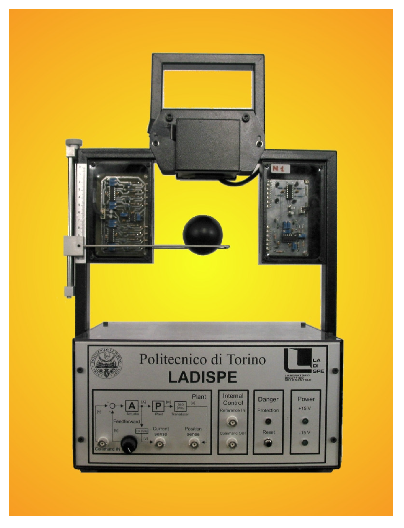
In this section, we apply the proposed control design technique to design a controller for the magnetic levitation system shown in Figure 10.

Figure 10. Magnetic levitation system.

In this system, a transconductance amplifier regulates the current through an electromagnet coil proportional to the input voltage u. The magnetic field, generated by the current, exerts a force on a light ball in the opposite direction to the gravity force. An optical transducer measures the ball position and produced the output voltage signal y. The book [47] provides a detailed description of the considered system. Magnetic levitation systems are highly non-linear unstable systems. In order to design a low order fixed structure controller, the control schema depicted in Figure 1 is considered, where a $G_n\left(s\right)$ is the linearized model of the magnetic levitation system obtained around a suitable equilibrium point and is given by

$$G_n\left(s\right)=\frac{Y\left(s\right)}{U\left(s\right)}=\frac{-7044}{(s-29.68)(s+29.68)}$$

(66)

where $U\left(s\right)$ and $Y\left(s\right)$ are the Laplace transform of the input and output voltage signals, respectively. It is worth noting that we consider the voltage transducer signal as system output to have a comparable reference signal w that can be produced by a common laboratory equipment, i.e., a signal generator. Moreover, we can directly measure the output voltage y with an oscilloscope, while the ball position in meters can be only computed through the knowledge of the mathematical model of the position transducer.

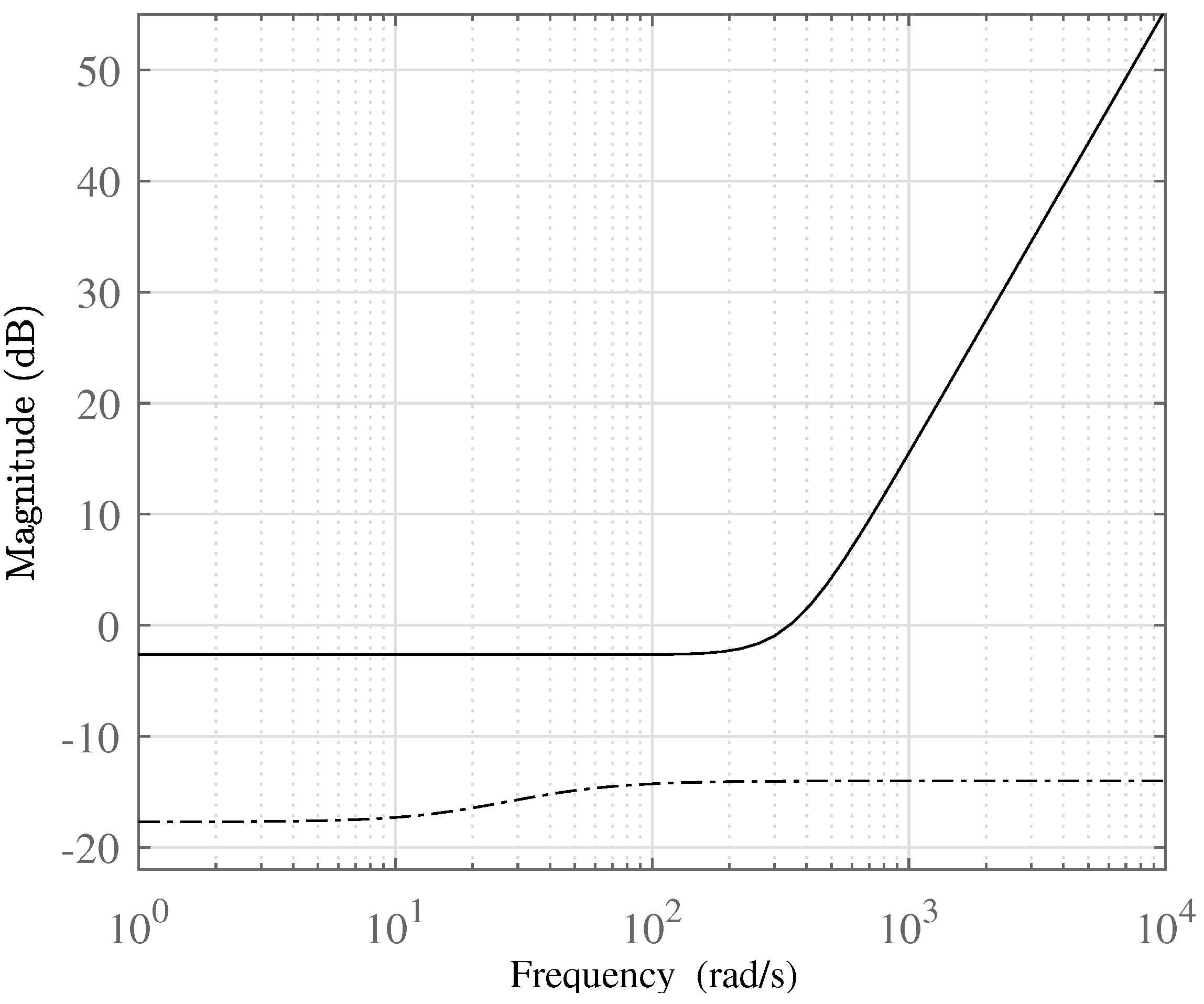
The nominal plant in Equation (66) is subjected to multiplicative uncertainty characterized by the following weighting function

$$W_u\left(s\right)=\frac{0.1993s^2+6.852s+55.96}{s^2+46.15s+429.5}.$$

(67)

The aim is to design a controller in the form

$$K(s,\mathit{p})=\frac{c_1{s}^2+c_{2}s+c_3}{c_4{s}^2+s},$$

(68)

where $p={[c_1,c_2,c_3,c_4]}^T\in R^4$ is the unknown parameter vector, such that the closed loop system is internally stable. Moreover, for a square wave reference signal $w\left(t\right)$ with period 2 s, duty-cycle $50\%$ and amplitude $0.1$ V, the closed loop system must satisfy the following nominal specifications: (i) zero steady-state tracking error for a step reference, (ii) rise time $t_r\le 0.015$ s, and (iii) overshoot $\widehat{s}\le 25\%$. The presence of a pole at $s=0$ in $K(s,\mathit{p})$ guarantees that the first requirement is implicitly achieved. According to the methodology described in [4], the time domain requirements are mapped into the frequency domain weighting filters

$$W_1\left(s\right)=\frac{s^2+145s+9877}{s(1.646s+82.3)}$$

(69)

and

$$W_2\left(s\right)=\frac{0.003333s^2+1.633s+414}{560.7}.$$

(70)

The constraints that define the stabilizing controller parameters set $\mathcal{S}$ are obtained by the Routh’s stability criterion, leading to

$$\begin{array}{cc}\hfill & g_1\left(p\right)=c_4>0\hfill \\ \hfill & g_2\left(p\right)=-140.88c_3>0\hfill \\ \hfill & g_3\left(p\right)=c_2{c}_4-c_1>0\hfill \\ \hfill & g_4\left(p\right)=c_1-c_2{c}_4-7.9963c_2^2{c}_4+7.9963c_1{c}_2+0.0011c_3>0.\hfill \end{array}$$

(71)

Since the magnetic levitation system is unstable, to avoid unstable pole-zero cancellation between the plant and the controller we consider stable $N_k(s,\mathit{p})$ and $D_k^{{}^{\prime }}(s,\mathit{p})$, where

$$N_k(s,\mathit{p})=c_1{s}^2+c_{2}s+c_3$$

(72)

and

$$D_k^{{}^{\prime }}(s,\mathit{p})=c_{4}s+1$$

(73)

Stability of $N_k(s,\mathit{p})$ and $D_k^{{}^{\prime }}(s,\mathit{p})$ is ensured by exploiting Routh Hurwitz criterion which provide following additional constraints in set $\mathcal{S}$.

$$\begin{array}{cc}\hfill & g_7\left(p\right)=-c_1>0\hfill \\ \hfill & g_8\left(p\right)=-c_2>0\hfill \end{array}$$

(74)

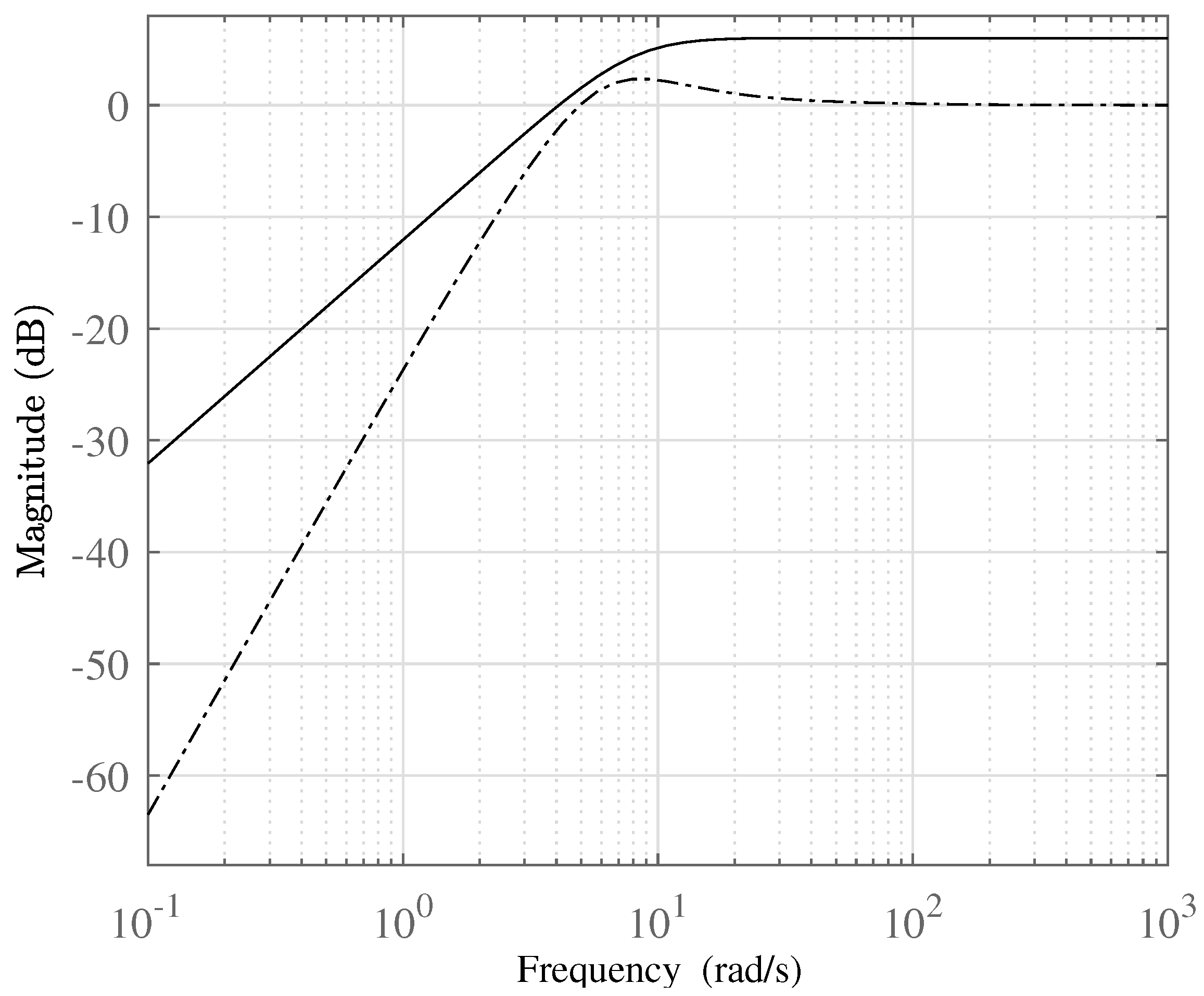
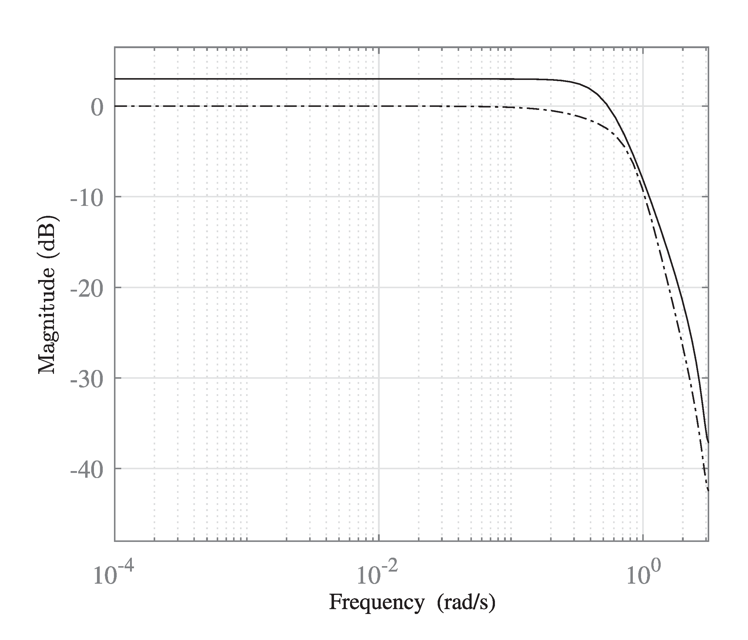
The graphical comparison between $W_2\left(s\right)$ and $W_u\left(s\right)$ is reported in Figure 11. Since $|W_2\left(s\right)|>|W_u\left(s\right)|$, we choose

$$\widehat{W_2}\left(s\right)=W_2\left(s\right).$$

(75)

Figure 11. Comparison between $|W_u\left(j\omega \right)|$(dotted) and $|W_{d2}\left(j\omega \right)|$ (solid).

The performance set $\mathcal{P}$ is derived in the same way as in previous examples. Through Result 11, we formulate the controller design as a SDP optimization problem by setting the relaxation order $\delta =1$ and $\Omega =[0,{10}^5]$. The relaxed SDP problem is solved with Yalmip (see [45]) and Mosek (see [46]). The controller extracted from the feasible controller parameters set is

$$K\left(s\right)=\frac{-0.0265s^2-1.226s-15.01}{0.0015s^2+s}.$$

(76)

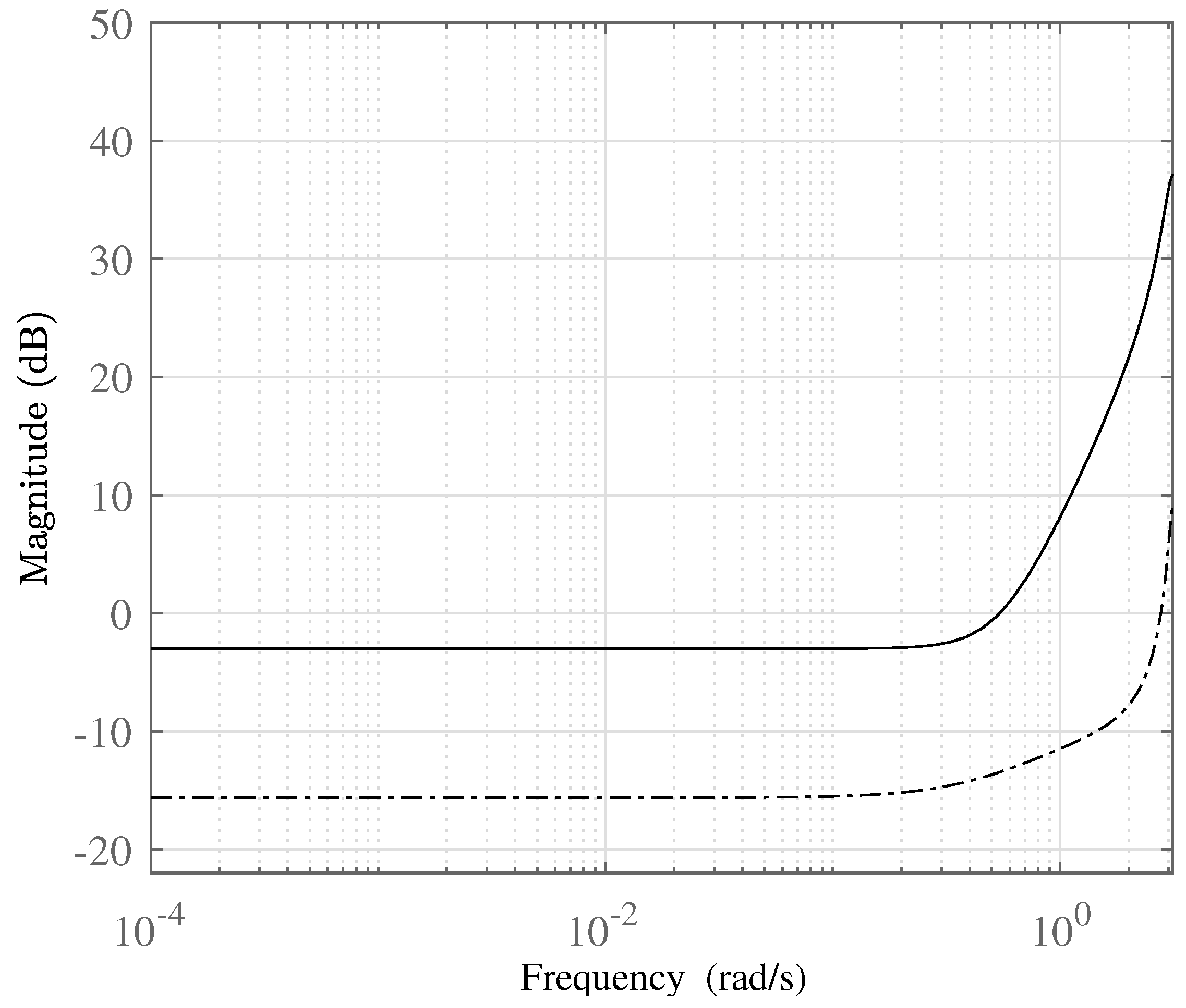
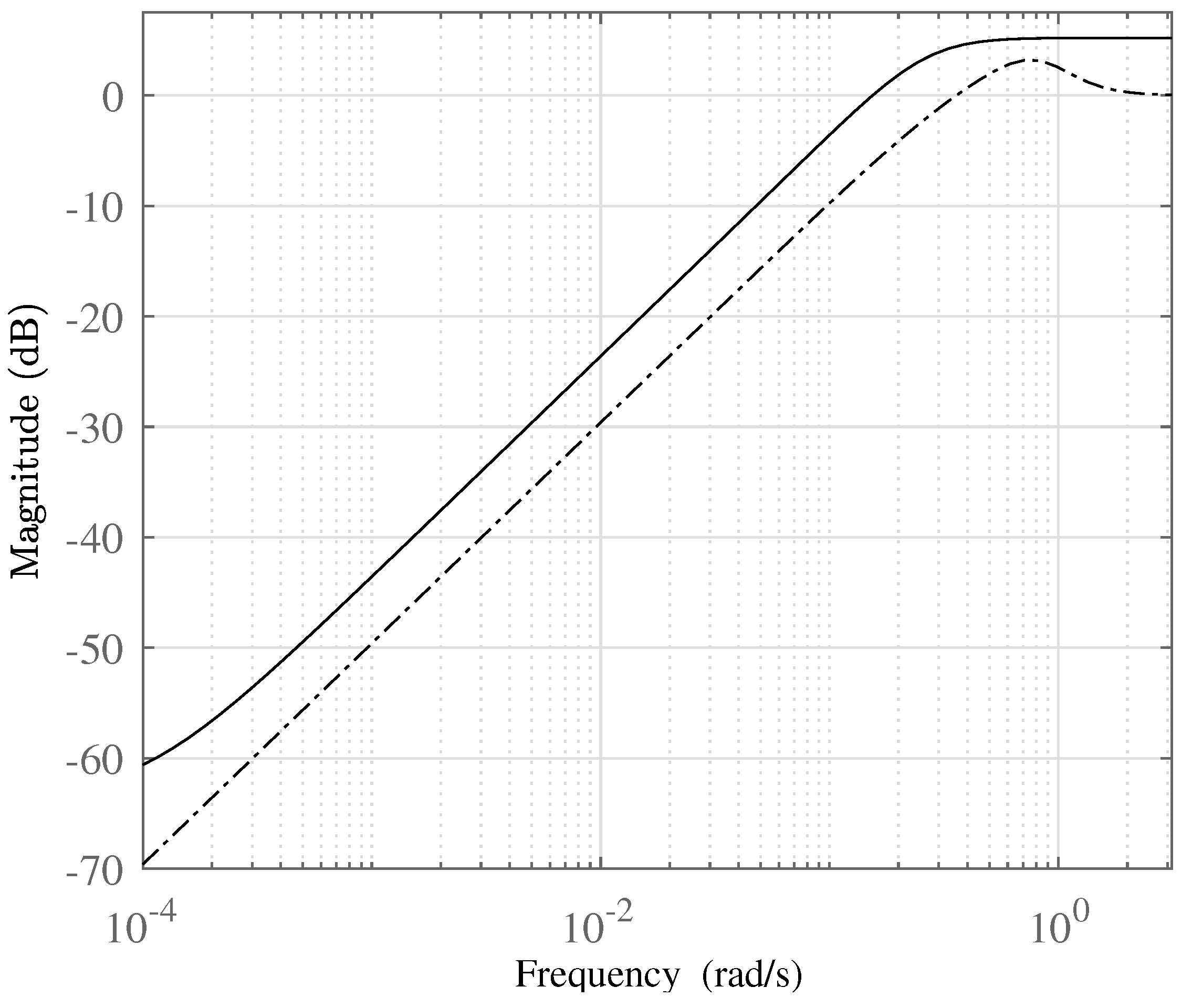
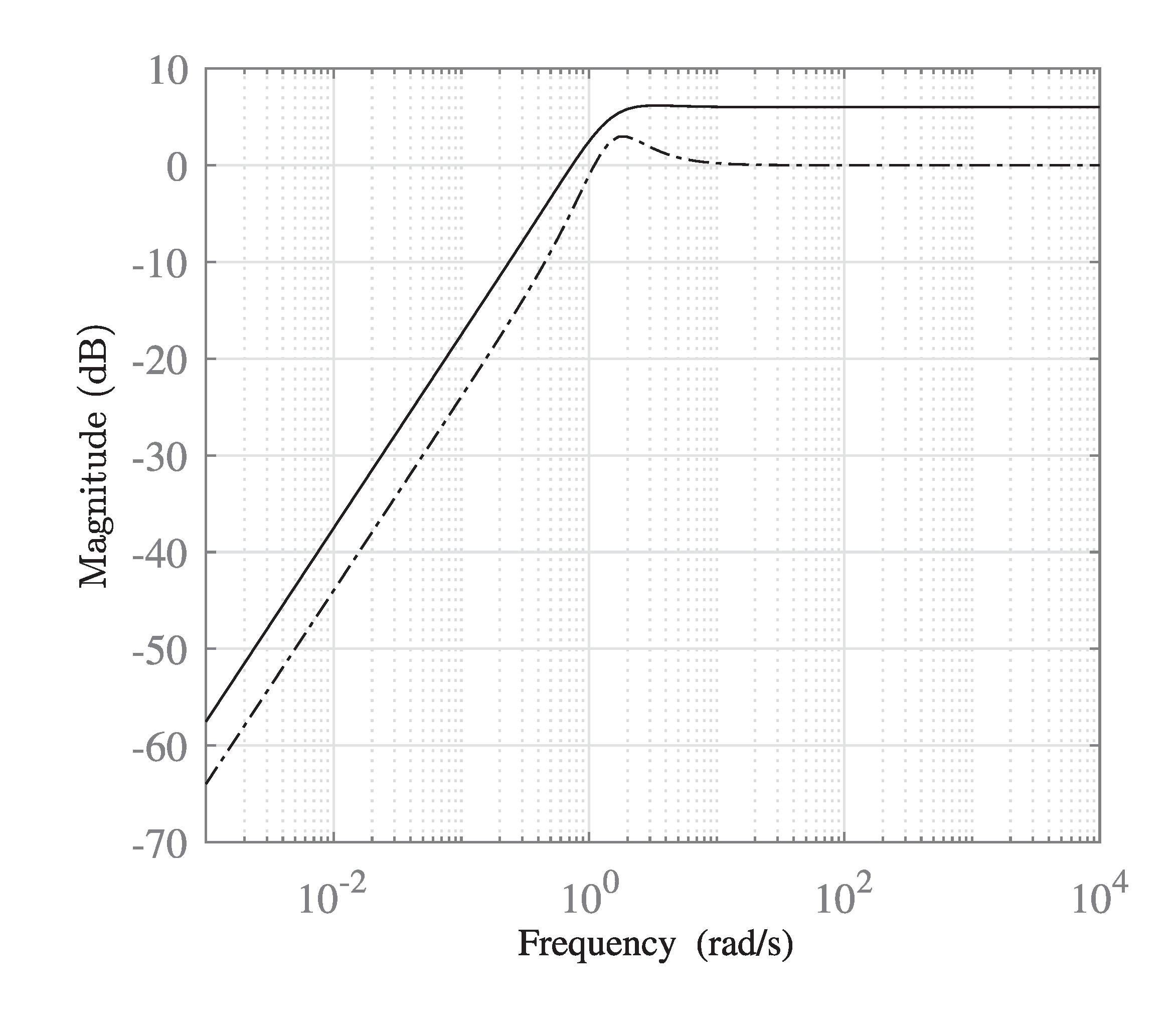
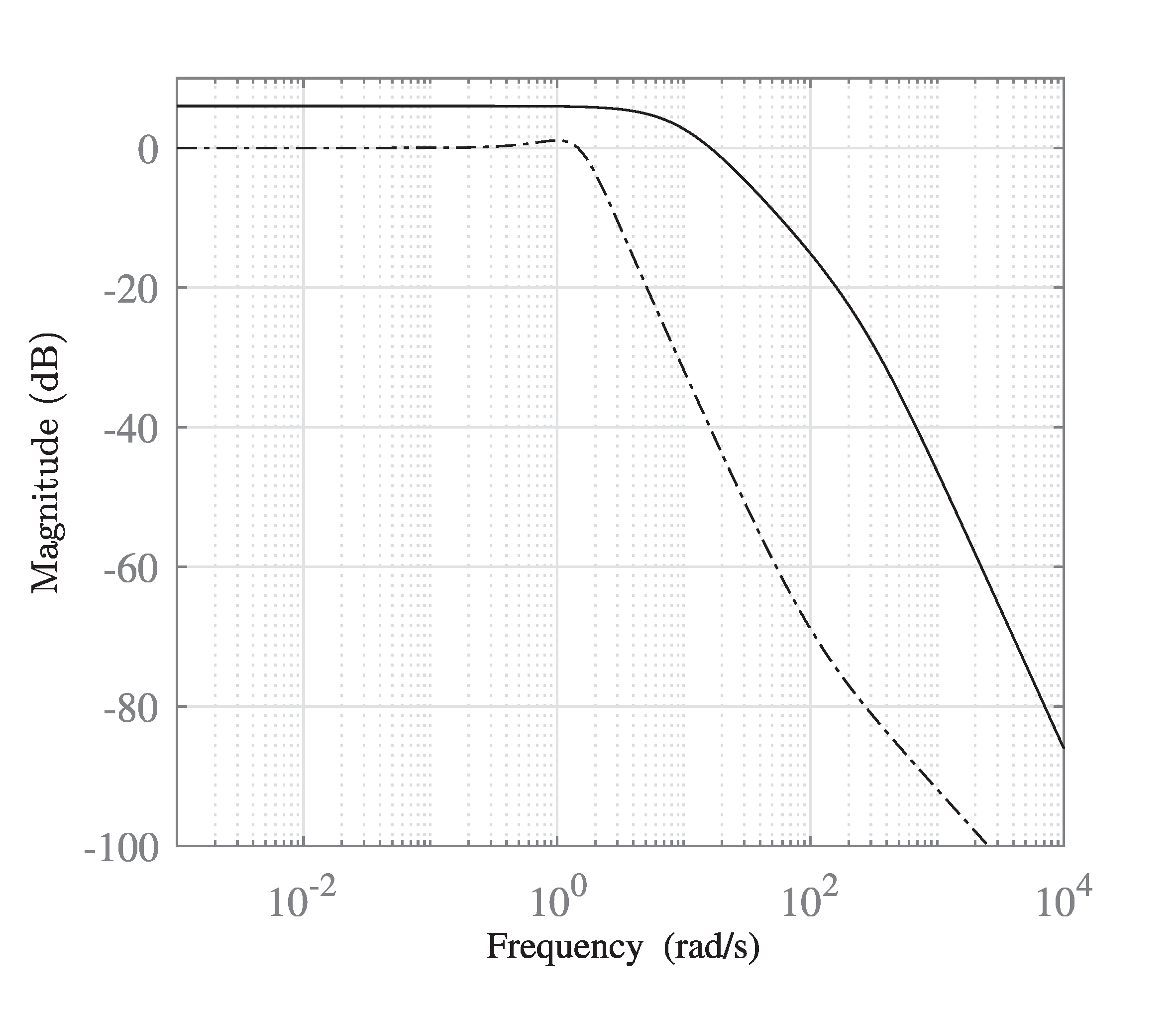
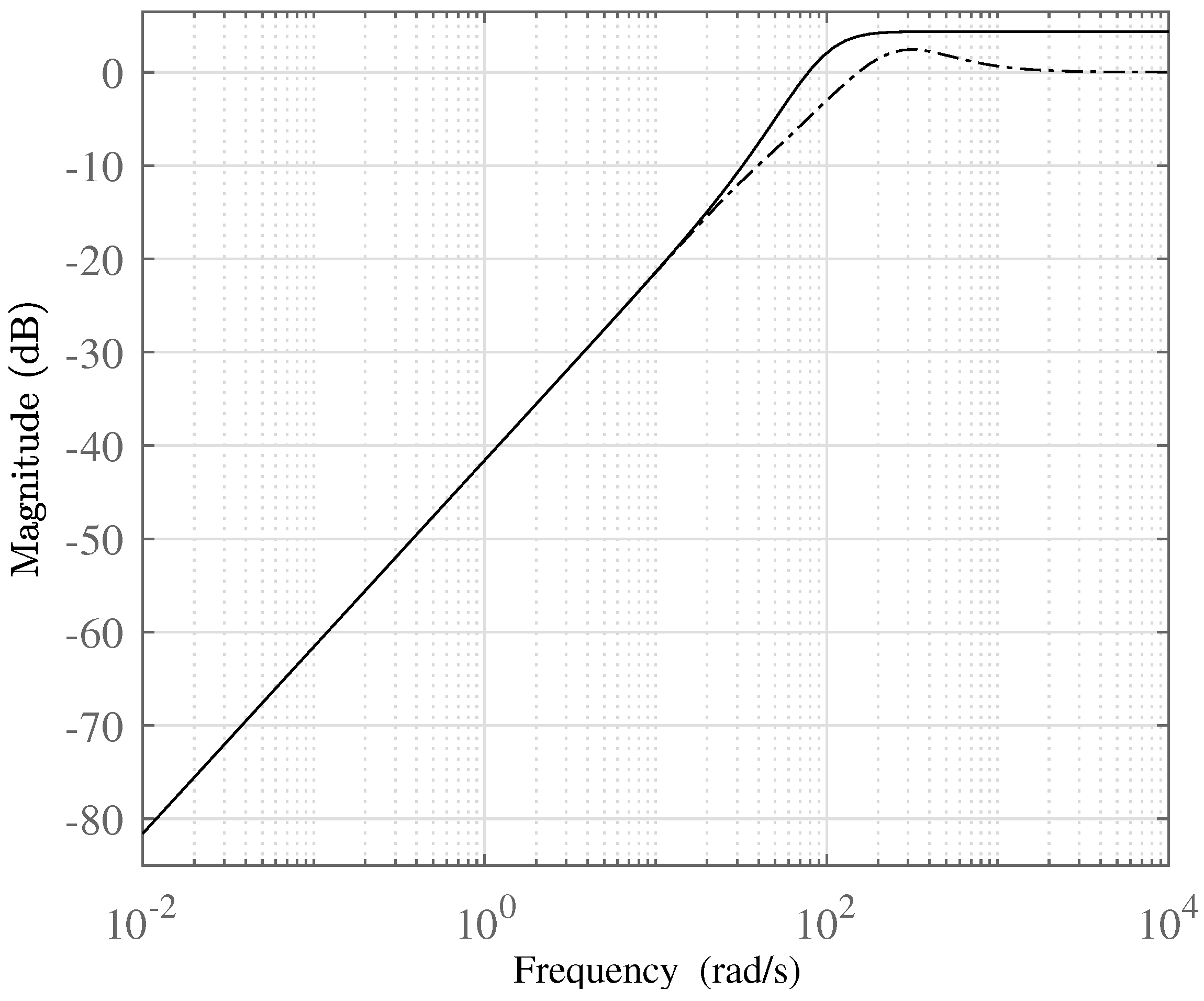
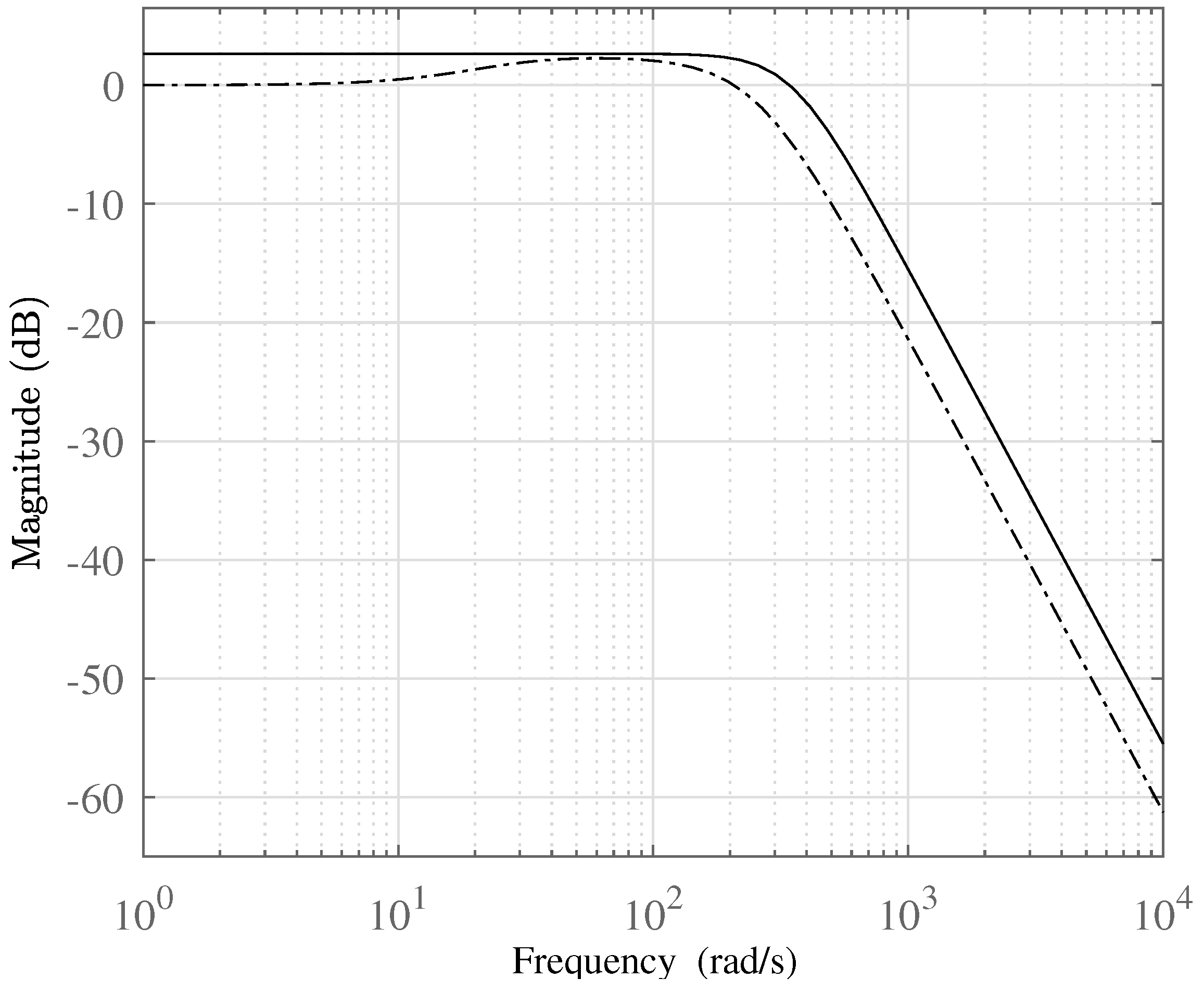
The controller achieves the nominal performances as $S_n\left(j\omega \right)$ and $T_n\left(j\omega \right)$ are smaller than $W_1\left(j\omega \right)$ and $W_2\left(j\omega \right)$, respectively (see Figure 12 and Figure 13). Numerically, $\parallel S_n\left(j\omega \right)W_1{\left(j\omega \right)\parallel }_{\infty }$ = 0.99 and $\parallel T_n\left(j\omega \right)W_2{\left(j\omega \right)\parallel }_{\infty }=0.9473$. 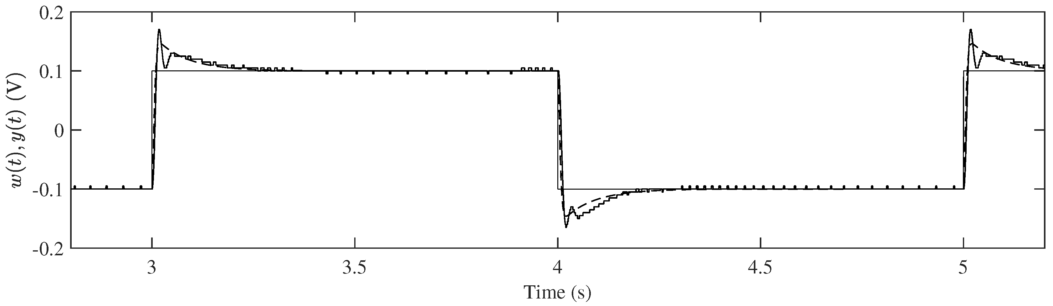We provide the comparison between the linearized system $G_n\left(s\right)$ and the real plant in Figure 14, which shows the time-domain responses of the closed-loop systems when the reference is a square wave with amplitude $0.1$V and frequency $0.5$ Hz. The linear system $G_n\left(s\right)$ achieves the time domain requirements: both the rise time $t_r\approx 0.00928$ s and the overshoot $\widehat{s}\approx 23.02\%$. However, the designed controller is not able to achieve the maximum overshoot requirement on the real plant, which is $\widehat{s}\approx 35\%$. The larger overshoot is due to the model mismatch between the non-linear plant and the approximated linear model and, thus, does not depend on the specific approach proposed in this work. Despite this modeling error, the designed controller stabilizes the magnetic levitation system and guarantees the rise time $t_r\approx 0.011$ s.

Figure 12. Comparison between $|W_1^{-1}\left(j\omega \right)|$ (solid) and $|S_n\left(j\omega \right)|$ (dotted).

Figure 13. Comparison between $|W_2^{-1}\left(j\omega \right)|$ (solid) and $|T_n\left(j\omega \right)|$ (dotted).

Figure 14. Magnetic levitation system response to square wave reference signal: reference $w\left(t\right)$ (solid square-wave), magnetic levitation system output $y\left(t\right)$ (solid) and linearized $G_n\left(s\right)$ system output (dashed) responses.

7. Conclusions

In this paper, we present a unified approach to design for the $H_{\infty }$ mixed-sensitivity design for fixed structure robust controllers for both CT and DT systems. We define the feasible controller parameter set as a semi-algebraic set of all the controller parameters that achieve nominal performance and robust stability for the closed-loop system. We formulate the control design problem as the non-emptiness test of the feasible controller parameters set, which is an NP-hard problem. Thanks to the results on the Putinar positivstellensatz, we propose a novel SOS based approach to formulate a convex relaxation of the original problem in terms of SDP constraints. Therefore, the achieved solution is not affected by local minima that may be found while solving non-convex problem through iterative methods. The proposed approach is a global optimization approach and is a powerful tool for fixed structure $H_{\infty }$ mixed sensitivity control design, whose solution can be found efficiently in polynomial time.

We provide three simulation examples and one experimental application to show the efficiency of the proposed algorithm on both CT and DT systems. In particular, one example shows the comparison of the proposed approach with the state of the art algorithm implemented in the Hinfstruct Matlab function. In this example, we show that the solution provided by Hinfstruct does not achieve the desired requirements, while our approach successfully solves the control design problem.