Abstract
Two-dimensional pumps have broad application prospects in aerospace. However, the performance of the pump is degraded because of the clearance problem of the current 2D transmission mechanism. In order to eliminate the clearance between the cam rail and the rollers, a high-speed transmission mechanism with a stacked roller set is proposed. The stacked roller set is compressed by the load pressure. The axial inertia force is balanced when the transmission mechanism works at high speed, via the equal acceleration and reverse movement of two cam rail sets. Thus, the transmission mechanism meets the high-speed demand. In this paper, the mathematical model of the transmission mechanism is established based on the enveloping surface theory and the differential geometry principle. Afterwards, numerical analysis of the mathematical model is performed based on MATLAB, combined with the experiment, to study the influence of load pressure and rotational speed on the torque loss. Then, the torque characteristics of the transmission mechanism is obtained. According to a test, the deviation between theoretical data and experimental data is 11.9%; therefore, the mathematical model can predict the torque of the transmission mechanism effectively. It is concluded that the torque loss of the transmission mechanism increases linearly with the load pressure, and the rotational speed has a slight effect on the torque loss.
1. Introduction
Axial piston pumps are widely used in aerospace by virtue of their high power density, strong load capacity and long service life [1,2]. Since the invention of axial piston pumps, their structure has been continuously optimized. However, there has never been a breakthrough in the overall architecture [3,4]. The high-speed performance of axial piston pumps is limited by three key friction pairs and overturning moment [5,6,7]. Therefore, the power-to-weight ratio of axial piston pumps cannot be further improved. In view of the defects of axial piston pumps, Ruan et al. [8] proposed a 2D piston based on the 2D hydraulic component concept. The rotational motion and reciprocating linear motion are designed on a single piston, which achieves a high integration of oil discharge and distribution, so as to design hydraulic pumps with a high power-to-weight ratio. The two-degree-of-freedom movement of the 2D piston is realized via a 2D transmission mechanism. Thus, the performance of the 2D pump will be impacted greatly by the high-speed performance, load capacity and stability of the 2D transmission mechanism.
The overall architecture of the 2D transmission mechanism is mainly built of spatial conjugate cam. It includes the fork assembly, the roller set and the cam rail set, as shown in Figure 1a. The fork assembly is driven by a motor to make the roller set rotate. Then, the roller set undergoes axial reciprocating movement under the constraint of the cam rail set. The 2D piston is connected to the roller set and moves with the roller set. Based on the above architecture, Tong et al. [9] designed a 2D hydraulic unit pump, which realizes the integration of oil discharge and distribution through the two-degree-of-freedom movement of the piston. Shentu et al. [10] adopted dual 2D pistons to reduce the flow ripple of the 2D pump substantially. Jin et al. [11,12,13] proposed an error compensation method for the cam rail surface, which decreased the contact clearance between the rollers and the cam rail. Qian et al. [14] analyzed the volumetric efficiency of the 2D pump based on CFD, and proved that its volumetric efficiency was more than 90% via experiments. Huang et al. [15,16,17] proposed a 2D transmission mechanism with inertial force balanced, as shown in Figure 1b, which increased the rotational speed of the 2D pump to 8000 rpm successfully, achieving high speed preliminarily. Ding et al. [18,19] analyzed the oil churning loss of the roller set and cam rail set of the 2D transmission mechanism based on CFD, and carried out experiments to obtain the empirical formula of churning loss torque.
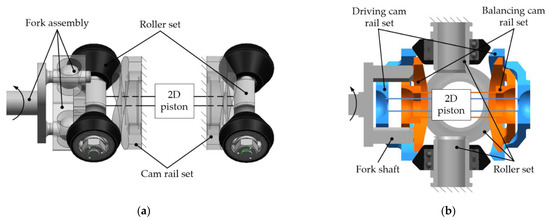
Figure 1.
Schematic diagram of the 2D transmission mechanism: (a) the overall architecture of the 2D transmission mechanism; (b) the 2D transmission mechanism with inertial force balanced.
The traditional 2D transmission mechanism fulfills the requirements of high load capacity and stability. However, the vibration caused by its axial inertial force will intensify with the increase in rotational speed, which limits the high speed. The 2D transmission mechanism with inertial force balanced eliminates the effect of the axial inertial forces, thereby achieving high speed. However, the clearance between the cam rail surface and the rollers cannot be eliminated, resulting in a loud noise and a decrease in mechanical efficiency of the 2D pump. In order to solve the clearance problem, this paper proposes a high-speed transmission mechanism with a stacked roller set, which improves the load capacity and power density of the 2D transmission mechanism, as well. The load pressure is used to compress the cone rollers of the transmission mechanism. Through adjusting the load pressure, the clearance can be effectively eliminated, the load capacity of the stacked roller set can be considerably improved by changing the compressing area and the number of the stacked rollers can grow within a certain range, thereby increasing the working frequency of the 2D piston, so as to meet the demand of high power-to-weight ratio of hydraulic components.
The rest of this paper is organized as follows. In Section 2, the structure and working principle of high-speed transmission mechanism with a stacked roller set is introduced. In Section 3, the accurate mathematical model is established based on the enveloping surface theory and differential geometry principle. In Section 4, numerical analysis is carried out based on MATLAB to study the influence of load pressure and rotational speed on the torque loss. In Section 5, a test rig is designed to measure the torque of the transmission mechanism. Afterwards, theoretical results are compared with experimental results. Finally, some useful conclusions are drawn in Section 6.
2. Structure and Working Principle
The high-speed transmission mechanism with a stacked roller set consists of a cross shaft, a stacked roller set, a roller casing, the cam rail set I and the cam rail set II. Its structure is shown in Figure 2. Among them, the stacked roller set, the cam rail set I and the cam rail set II are the core components that realize the conversion of rotation and linear motion.
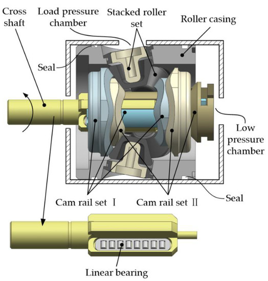
Figure 2.
Structure of the high-speed transmission mechanism with a stacked roller set.
The stacked roller set is composed of N cone roller components in a specific geometric law. Each cone roller component consists of a roller ring, a roller shaft and a cone roller. The front view of the stacked roller set is shown in Figure 3a. The cone rollers contact in pairs. All contact lines lie in the same plane and intersect at the center O. Figure 3c shows the projection of the contact lines on the bottom of the cone roller. The N cone rollers are alternately arranged on both sides of the contact plane. Their axes form an angle γ with the contact plane, as shown in Figure 3b. The specific geometric law of the N cone rollers satisfies the Equation (1):
where α is the angle between two adjacent contact lines, N is the number of cone rollers, β is the half cone angle of the cone roller, b is the angle between the projection lines of two adjacent contact lines and γ is the angle between the axis of the cone roller and the contact plane.
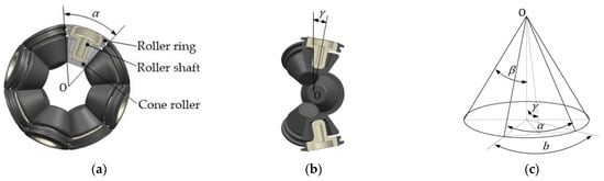
Figure 3.
Structure principle of the stacked roller set: (a) front view of the stacked roller set; (b) side view of the stacked roller set; (c) projection of the cone roller.
The cam rail set I is composed of an outer cam rail I, an inner cam rail I and an inner fork shaft, as shown in Figure 4a. The outer cam rail I and inner cam rail I are a pair of conjugate end cams. The cam surface is formed of equal acceleration and deceleration curves with N/2 cycles. Its motion law is shown in Figure 5. The two cam rails are installed on the inner fork shaft in the way of peak corresponding to peak. The side wall of the inner fork shaft is in contact with the cross shaft and the locking structure at the right end is used to connect the 2D piston. The structure of the cam rail set II is similar to that of the cam rail set I, as shown in Figure 4b. However, the installation phase of the two is different, whose angle difference is 2π/N in the way of peak corresponding to trough.

Figure 4.
Schematic diagram of cam rail sets: (a) structure of the cam rail set I; (b) structure of the cam rail set II.
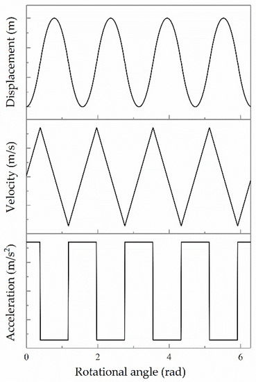
Figure 5.
The motion law of the cam rail set.
According to Figure 2, when the transmission mechanism works, the cross shaft, as the input shaft, drives the two cam rail sets to rotate synchronously by contacting the side walls of the inner and outer fork shafts through the linear bearing. The load pressure chamber is filled with high-pressure oil, which is on the outside of the roller casing. High-pressure oil creates a pressure difference with the low pressure chamber inside, pressing the large end of the roller shaft, so that the N cone rollers are attached to the cam rail surface closely. In addition, the parts are lubricated by the low-pressure oil in the low pressure chamber. Afterwards, the cam rails are constrained by the stacked roller set, which forces the cam rail sets to move in equal acceleration and deceleration reciprocating linear motions. Since the installation phases of the two cam rail sets are different, the two cam rail sets will drive their respective 2D pistons to move in reverse reciprocating linear motions. The 2D pistons also moves in rotational motions synchronously, so as to realize the conversion and integration of two-degree-of-freedom motions.
3. Mathematical Model
In this section, the cam rail surface equation of the high-speed transmission mechanism with a stacked roller set is established based on the enveloping surface theory. The space vectors are derived at the contact points to calculate the space angles of forces. Eventually, the accurate dynamic equations are established to provide a mathematical model for numerical analysis.
3.1. Cam Rail Surface Equation
In order to parameterize the surface of the cam rail and cone rollers, the global coordinate system O0−X0Y0Z0 and the moving coordinate system O3−X3Y3Z3 are first set up. The reference frame is shown in Figure 6. The axis Z0 of the coordinate system O0−X0Y0Z0 is collinear with the rotational axis of the cam rail. The axis Z3 of the coordinate system O3−X3Y3Z3 is collinear with the rotational axis of the cone roller. In addition, the origin O3 located at the axis Z0 coincides with the vertex of the cone roller. To describe the spatial relationship between the cone roller and the cam rail via homogeneous coordinate transformation, the relative coordinate systems O1−X1Y1Z1 and O2−X2Y2Z2 are set up. The coordinate system O1−X1Y1Z1 is obtained by the translation of the coordinate system O0−X0Y0Z0 along the axis Z0. The coordinate system O2−X2Y2Z2 is obtained by the rotation of the coordinate system O1−X1Y1Z1 around the axis Z1. Moreover, the coordinate system O3−X3Y3Z3 is obtained by the rotation of the coordinate system O2−X2Y2Z2 around the axis X2, where the rotational angle is π/2−γ.
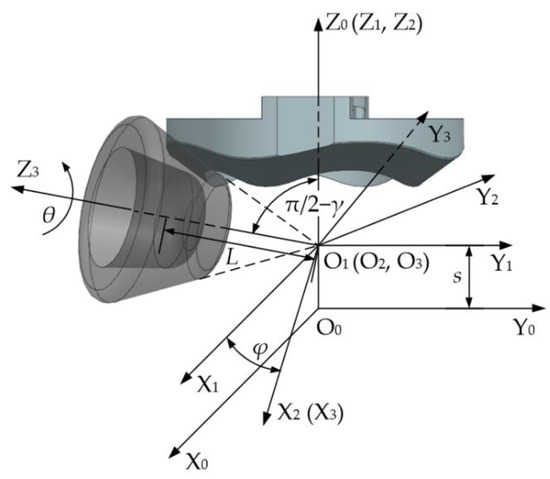
Figure 6.
Reference frame.
The cam rail surface is constructed by equal acceleration and deceleration curves with N/2 cycles. Therefore, it is available to perform a circular array to create a complete cam rail surface by deriving the single-cycle surface equation. Thus, the displacement s can be described as:
where s is the axial displacement of the cam rail, h is the stroke of the cam rail and φ is the rotational angle of the cam rail.
According to the parameters and coordinate systems set above, the cone roller surface in the moving coordinate system can be described as:
where L is the distance from any point on the surface of the cone roller to the plane X3O3Y3 and θ is the rotational angle of the cone roller.
The transformation matrix from the coordinate system O0−X0Y0Z0 to the coordinate system O1−X1Y1Z1 can be expressed as:
The transformation matrix from the coordinate system O1−X1Y1Z1 to the coordinate system O2−X2Y2Z2 can be expressed as:
The transformation matrix from the coordinate system O2−X2Y2Z2 to the coordinate system O3−X3Y3Z3 can be expressed as:
Via homogeneous coordinate transformation, the expression of the cone roller surface can be transformed into the single-parameter equation of surface family of the cone roller in the global coordinate system [20], which can be described as:
Based on the enveloping surface theory of single-parameter surface family [21], the equation can be written as a vector function . Aiming to derive the equation of the cam rail surface, it is necessary to require the vector function to satisfy the constraint Equation (8):
Equation (9) can be acquired by solving the constraint equation, which can be expressed as:
Equation (9) indicates the contact relationship between the cam rail surface and the cone roller surface. By substituting Equation (9) into Equation (7), the parametric expression of the cam rail surface can be obtained, which is denoted as:
3.2. Space Angle Functions
On the basis of the parametric cam rail surface and the differential geometry principle, the tangent vectors, the normal vectors and their projections on the bottom of the cone roller can be obtained at the contact points. The space angle functions of the vectors are derived with auxiliary vectors, which take the rotational angle φ and the distance L as variables. Then, the directions of the forces are determined in the global coordinate system.
As for the single-parameter surface family, the tangent vector at any point on the surface of the cone roller is the partial derivative of the vector function with respect to the parameters θ and L, which are and . Among them, the tangent vector represents the direction of the circumferential friction acting on the cone roller, and the tangent vector represents the direction of the sliding friction along the generatrix of the cone roller. The normal vector of the cone roller surface can be obtained by the cross product of the tangent vectors and , namely . Afterwards, the direction of the normal force acting on the cone roller surface can be determined through the normal vector. Additionally, the direction of the component of the normal force can be obtained by projecting the normal vector on the bottom of the cone roller, which is denoted as .
In order to facilitate the decomposition of forces, referring to Figure 6, the unit vector is set along the circumference of the cam rail at the contact points. The unit vector in the global coordinate system is transformed from the unit vector of the axis Y3. The unit vector of the axis Z0 in the global coordinate system is denoted as , so as to indicate the axial direction of the cam rail.
According to the scalar products of the above space vectors, the functions of space angles with respect to the rotational angle φ and the distance L can be obtained by utilizing Equation (9) to eliminate the parameter θ. Therefore, the function of the pressure angle of the cam rail surface can described as:
The function of the acute angle , which indicates the angle relationship between the friction and the axial direction of the cam rail, can be described as:
The function of the acute angle , which represents the angle relationship between the normal force and the circumferential unit vector at the contact point, can be described as:
The function of the acute angle , which indicates the angle relationship between the friction and the circumferential unit vector at the contact point, can be described as:
The function of the space angle , which represents the angle relationship between the component of the normal force and the axis Y3, can be described as:
3.3. Dynamic Equilibrium Equations
The mechanical behavior of the stacked roller set and the cam rail sets is very complicated, so the mechanical model needs to be simplified. According to the structural characteristics of the cam rail surface, the cam rail set can perform N/2 reciprocating linear movements per revolution. During each revolution, the phase difference is 2π/N between the outer cam rail and the inner cam rail. Therefore, the numerical analysis can be performed in 1/2 working cycle, which is the working section of in the Equation (2). Since the contact line of the cone roller with the cam rail is a complex space curve which cannot be integrated, the distributed forces need to be simplified to the concentrated force at the midpoint of the contact line. Taking into account that the transmission mechanism can eliminate the clearance, the inner and outer cam rails must be always in contact with the stacked roller set, so the inner and outer cam rails must be always under force.
According to the above premise, assuming that the cam rail set I is moving to the right, the acceleration can be expressed as:
where n is the rotational speed of the cam rail set.
As shown in Figure 7, the displacement s and the rotational angle φ are taken as generalized coordinates. Then, the dynamic equilibrium equations are established in these two coordinates. It is supposed that the instantaneous torque of the transmission mechanism is , so the input torque of the cam rail set I will be . The input torque acts on the side walls of the inner fork shaft and generates friction . The outer cam rail I is subjected to the normal force and the friction of the stacked roller set, and its outer peripheral surface is subjected to the oil stirring shear moment at the same time. The inner cam rail I is subjected to the normal force and the friction of the stacked roller set. Since the rotational speeds of the inner and outer cam rails are the same, the oil stirring shear moment can be ignored, which is caused by the relative movement of the inner and outer cam rails. The space angles of the forces acting on the outer cam rail I correspond to the space angle functions mentioned in the previous section, because the outer cam rail I is in the returning stroke, which means that the cone roller works in the thrusting stroke. On the contrary, since the inner cam rail I is in the thrusting stroke, the phase difference of its space angle functions is 2π/N. Considering the number of the cone rollers, the forces acting on the cam rail need to be multiplied by N/2. In summary, the two dynamic equilibrium equations can be derived as:
where , , is the mass of the cam rail set I, is the force arm of the normal force and the friction , is the force arm of the normal force and the friction , , and .
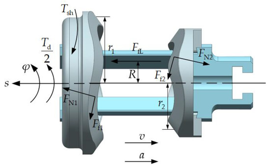
Figure 7.
Force analysis of the cam rail set I.
As shown in Figure 8, the forces acting on the cam rail set II is almost the same as mentioned above. The outer fork shaft is subjected to the input torque and the friction . The inner cam rail II is subjected to the normal force and the friction of the stacked roller set. The outer cam rail II is subjected to the normal force and the friction of the stacked roller set. Meanwhile, the outer peripheral surface of the outer cam rail II is subjected to the oil stirring shear torque . Among them, the magnitude of the normal force is equal to that of the normal force , and the magnitude of the normal force is equal to that of the normal force . Thus, the frictions corresponding to them are respectively equal.
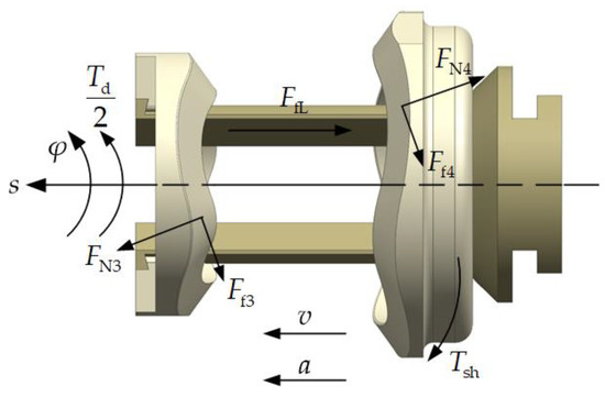
Figure 8.
Force analysis of the cam rail set II.
As shown in Figure 9a, the stacked roller set is subjected to the counterforces of the inner and outer cam rails and the oil load pressure. Now, the arbitrary cone roller on the right side is picked for force analysis. The cone roller is subjected to the counterforces, , , and , of the inner cam rail I and outer cam rail II. It is also subjected to the normal forces, and , of the left cone rollers. The cone roller is supported by the supporting force of the roller shaft and affected by the friction torque . Consequently, the dynamic equilibrium is realized. In order to simplify the model, it is supposed that the normal forces, and , are equal. What is more, the supporting force is located in the plane xOz, and the direction vector of it forms an angle ϕ with the axis z. In detail, the coordinate system O-xyz is obtained by translating the moving coordinate system along the axis Z3, whose origin is located at the center of the bottom of the cone roller. Thus, the dynamic equilibrium equation in the z-axis direction can be expressed as:
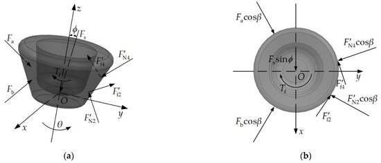
Figure 9.
Force analysis of the cone roller: (a) schematic diagram of the forces acting on the cone roller; (b) projection of the forces.
The projection of the forces on the bottom of the cone roller are shown in Figure 9b. Since the outer cam rail II is in the returning stroke, the space angles of the counterforces of it correspond to the angle functions mentioned in the previous section. On the contrary, the space angles of the counterforces performed by the inner cam rail I have a phase difference of 2π/N. Therefore, the dynamic equilibrium equation of the cone roller in the y-axis direction can be expressed as:
where .
In order to make the mathematical model easier to calculate, the formula is used to convert all the frictions into the product of the friction coefficient and the normal forces. The component of the supporting force in the z-axis direction is equal to the oil hydraulic load acting on the large end of the roller shaft. Hence, the pressing force is introduced into the model, namely , where p is the load pressure and A is the area of the large end of the roller shaft. It should be pointed out that the pressing force is offered by the pressure difference between the load pressure chamber and the low pressure chamber. The pressure difference can be substituted with the load pressure, because the pressure of the low pressure chamber is nearly zero. Eventually, Equations (17)–(20) are transformed into a matrix through the above conversion, which can be described as:
where R is the force arm of the friction .
According to the previous research [22], the formula of the oil stirring shear torque is given by the following Equation (22):
where µ is the dynamic viscosity of the oil, is the average diameter of the outer peripheral surface of the outer cam rail, is the average width of the outer peripheral surface of the outer cam rail and is the average gap between the outer peripheral surface of the outer cam rail and the inner wall of the roller casing.
By substituting Equations (11)–(16) and (22) into Equation (21), the functions of the forces , and and the instantaneous torque can be obtained with respect to the rotational angle φ, the load pressure p and the rotational speed n. Through discretizing the instantaneous torque function as well as discretizing the interval into a sequence (t is the spacing of the sequence), the average torque T can be obtained as a function of the load pressure p and the rotational speed n, which can be described as:
4. Numerical Analysis
According to the above mathematical model, numerical analysis is conducted based on MATLAB in this section. First of all, all the equations and formulas of the above mathematical model are programmed in MATLAB. The trend of the key forces with respect to the rotational angle and the load pressure is studied in the working section [0, 45°]. In the above model, the friction in the structure belongs to the sliding-rolling friction of steel to steel, which is dominated by rolling friction. Therefore, the range of the friction coefficient is roughly 0.001 to 0.02 [23]. The default value of the friction coefficient is supposed to be 0.007 here. Then, based on different friction coefficients, the influence of the load pressure and the rotational speed on the torque loss is discussed. The parameters for calculation are shown in Table 1.

Table 1.
Parameters for calculation.
4.1. Analysis of Key Forces
The key forces in the mathematical model refer to the normal forces , and and the instantaneous torque . Their trend characterizes the working characteristics of the cam rail sets and the stacked roller set with change in the rotational angle. In addition, their trend with the load pressure changing can indicate whether there is a clearance between the cone roller on a certain side and the cam rail. Thus, it is provable that the transmission mechanism has the capability to eliminate the clearance.
The designed limit of the rotational speed of the transmission mechanism is 10,000 rpm. The working condition will be the worst when the rotational speed achieves the limit. Hence, the limit can be used as a preset value for the following research. At different load pressures, the curves of the normal forces and with respect to the rotational angle are shown in Figure 10 and Figure 11. When the rotational angle changes from 0° to 22.5°, the cam rail set I is moving to the right with the equal acceleration. It is noticeable that the normal force is greater than the normal force to provide the acceleration to the right direction. When the rotational angle is equal to 22.5°, the normal forces and are both mutated due to the flexible impact of the equal acceleration and deceleration motion law. When the rotational angle changes from 22.5° to 45°, the cam rail set I is moving to the right with the equal deceleration. It is apparent that the normal force is greater than the normal force to provide the acceleration to the left direction. Moreover, the normal force is equal to 0 in the section that the cam rail set I moving to the right with the equal acceleration, when the load pressure is 1 MPa. Consequently, it indicates that the left cone rollers do not contact with the outer cam rail I. Thus, it can be deduced that there is a clearance between the left cone rollers and the outer cam rail I. When the normal force is equal to 0, it can be deduced that there is a clearance between the right cone rollers and the inner cam rail I, as well. When the load pressure is larger than 2 MPa, the normal forces and are positive, which means that the clearance has been eliminated. To be precise, the critical value is 1.60 MPa when the normal forces turn to positive throughout the certain working section.
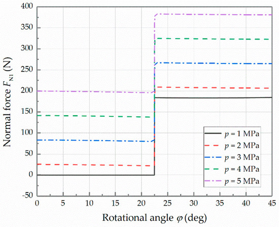
Figure 10.
Curves of the normal force at different pressures.
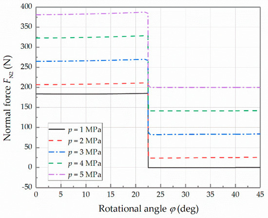
Figure 11.
Curves of the normal force at different pressures.
At different load pressures, the curves of the normal force with respect to the rotational angle are shown in Figure 12. In the stacked roller set, the normal forces among the cone rollers are relatively stable, which hardly change with the rotational angle. However, an increment of the load pressure will result in an increase in the normal force , which indicates that adjusting the load pressure can change the load capacity of the stacked roller set.
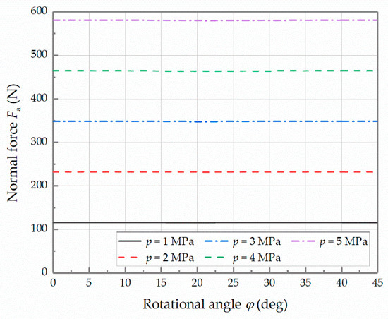
Figure 12.
Curves of the normal force at different pressures.
At different load pressures, the curves of the instantaneous torque with respect to the rotational angle are shown in Figure 13. When the rotational angle changes from 0° to 45°, the instantaneous torque increases to the peak value linearly at the beginning. At the point = 22.5° the instantaneous torque jumps to the trough value. Then, it linearly increases to the initial value again. It shows that the shape of the curves of the instantaneous torque is sawtooth in the complete working process. Compared with the rotational angle, the load pressure has little effect on the instantaneous torque.
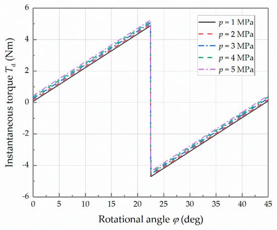
Figure 13.
Curves of the instantaneous torque at different pressures.
4.2. Analysis of the Torque Loss
Since the mathematical model describes the no-load situation, the average torque can characterize the torque loss of the transmission mechanism effectively. When the rotational speed is 10,000 rpm, the curves of the torque loss with respect to the load pressure and different friction coefficients are shown in Figure 14. According to Figure 14, increasing the load pressure can eliminate the contact clearance between the cone rollers and the cam rails. However, it also makes the components of the frictions and the normal forces become larger in the circumferential direction of the cam rail, resulting in an increase in the torque loss. The designed limit of the load pressure is 5 MPa. When the load pressure achieves the limit, the curves of the torque loss with respect to the rotational speed at different friction coefficients are shown in Figure 15. The increment in the rotational speed raises the torque loss slightly. The two figures reflect that the increment in the friction coefficient will lead to a substantial increase in the torque loss.
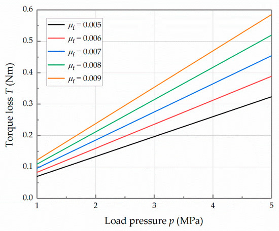
Figure 14.
Curves of the torque loss with respect to the load pressure at different friction coefficients.
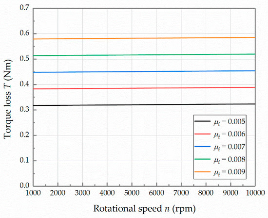
Figure 15.
Curves of the torque loss with respect to the rotational speed at different friction coefficients.
When the friction coefficient is equal to the preset value, which is 0.007, the function of the torque loss with respect to the load pressure and the rotational speed can be obtained according to Equation (23). The function can be expressed as:
Therefore, the theoretical torque characteristics of the transmission mechanism are shown in Figure 16. In the extreme case, the maximum axial load can reach 1150 N and the mechanical efficiency can reach 91.45% when the stacked roller set can be effectively compressed. It needs to be pointed out that the form of the load refers to that of the novel stacked rollers 2D piston pump [24].
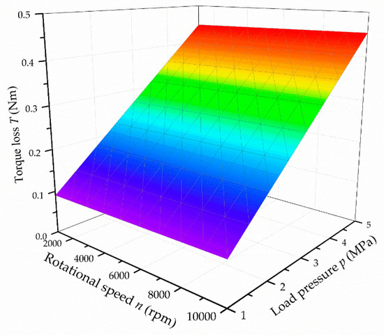
Figure 16.
Theoretical torque characteristics.
5. Experimental Research
In order to verify the correctness of the mathematical model and analytical results, an experiment rig is built to measure the torque of the high-speed transmission mechanism with a stacked roller set. The schematic diagram of the experiment rig is shown in Figure 17. The pumping station supplies the high-pressure oil for the load pressure. As the pressure of its returning oil can be regarded as zero, the pressure difference used to compress the stacked roller set can be equivalent to the pressure measured in the port of the load pressure chamber. A three-phase variable frequency motor is used to drive the transmission mechanism. The maximum rotational speed of the motor can reach 20,000 rpm. The pressure sensor is utilized to measure the load pressure, and the torque/speed sensor is used to measure the torque and rotational speed of the transmission mechanism. The load pressure, torque and rotational speed can be collected by the data acquisition card, and are processed through LabVIEW on the computer. The results are displayed on the screen for reading and recording. The details of the relevant sensors are shown in Table 2.
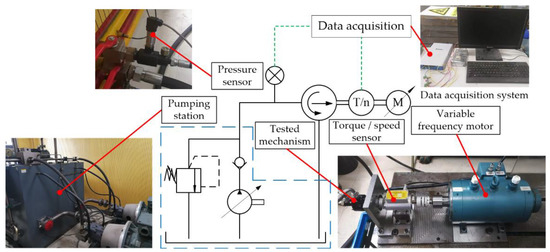
Figure 17.
Schematic diagram of the experiment rig.
Table 2.
Details of the relevant sensors.
Firstly, the motor is accelerated to 10,000 rpm, and the pressure sensor reading is adjusted to each target value via regulating the output pressure of the pumping station. When the torque display stabilizes, the data are recorded. The analytical and experimental torque losses with respect to the load pressure are shown in Figure 18. When the load pressure changes from 1 MPa to 5 MPa, the experimental torque loss is increasing linearly with the load pressure, which is consistent with the theoretical trend. The practical friction coefficient gradually raises from 0.005 to 0.008. The reason might be that the increase in the load pressure causes the enhancement of friction loss, which results in a temperature rise. Then, the viscosity of the oil drops, causing the lubrication to deteriorate. In general, the average friction coefficient of the transmission mechanism is about 0.007.
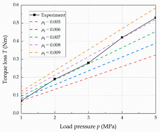
Figure 18.
Analytical and experimental torque losses with respect to the load pressure at the rotational speed of 10,000 rpm.
Secondly, the pressure sensor reading is adjusted to 5 MPa by regulating the output pressure of the pumping station, and the motor is accelerated to each target rotational speed. When the torque display stabilizes, the data are recorded. The analytical and experimental torque losses with respect to the rotational speed are shown in Figure 19. When the rotational speed raises from 1000 rpm to 7000 rpm, the torque loss has a slight increase, and its value remains approximately 0.45 Nm. While the rotational speed continues to raise to 10,000 rpm, the torque loss increases significantly, eventually reaching 0.53 Nm. The probable reason of the difference in the final stage is illustrated as following. Due to the temperature rise caused by the high speed, the lubrication effect deteriorates, which results in an increase in friction loss. Therefore, the higher speed leads to a larger torque loss.
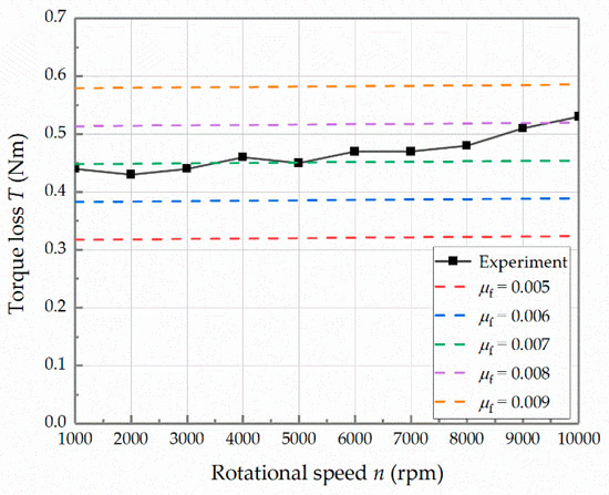
Figure 19.
Analytical and experimental torque losses with respect to the rotational speed at the load pressure of 5 MPa.
Finally, the pressure sensor reading is adjusted to each target value via regulating the output pressure of the pumping station, and the motor is accelerated to the target rotational speed at each load pressure. When the display is stable, the data are recorded. The operation is repeated three times. Afterwards, the mean values are calculated to draw the figures. The comparison of the practical and theoretical torque characteristics of the transmission mechanism are shown in Figure 20. The data from Figure 20 are listed in Table 3. Among them, the difference is largest when the load pressure is 1 MPa, because the torque loss is too close to the precision of the torque/speed sensor. It can be obtained that the mean error between the analytical results and the experimental results is 11.9%. Apart from the data when the load pressure is 1 MPa, the mean error can be much better, which is 8.9%.
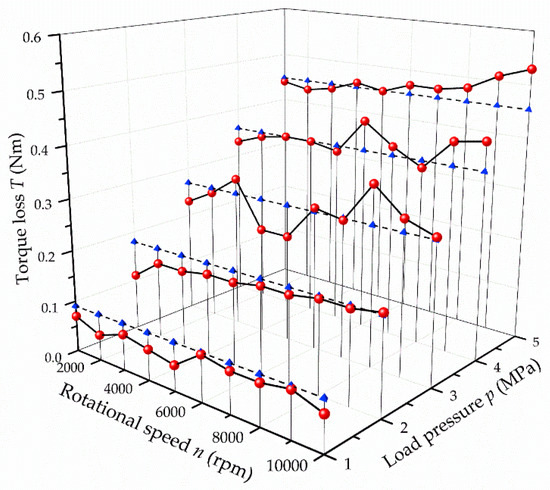
Figure 20.
Comparison of practical torque characteristics and theoretical torque characteristics.
Table 3.
Error between the practical torque loss and theoretical torque loss.
6. Conclusions
Firstly, this paper introduces the structure and working principle of the high-speed transmission mechanism with a stacked roller set. Secondly, the equation of the cam rail surface is established based on the enveloping surface theory. Then, the space angle functions of the forces are derived based on the differential geometry principle. Afterwards, the dynamic equilibrium equations are obtained. Eventually, the influence of the load pressure and the rotational speed on the torque loss is studied at different friction coefficients. The mathematical model was verified by the experiment. Some useful conclusions are drawn as follows:
- (1)
- According to the mathematical model, in the case of low load pressure, the normal forces, and , between the cam rail and the rollers have zero values. In this situation, there might be a contact clearance between the cam rail and the rollers on one side, which means it is invalid to press the stacked roller set to support the cam rail.
- (2)
- The validity of the mathematical model is verified by the experimental results. Combined the analytical results with the experimental results, the increment of the load pressure will enlarge the normal forces and the frictions, which raises the torque loss of the transmission mechanism significantly. Furthermore, the increase in the rotational speed will make the axial inertia forces of the cam rail sets increase. However, the influence of the rotational speed on the torque loss is slight, because the mass of the cam rail set is very small.
- (3)
- In the case of high speed and high pressure, the viscosity of the oil decreases due to the temperature rise, which leads to the deterioration of the lubrication. Therefore, there is a growing trend of the friction coefficient. Overall, the average friction coefficient of the transmission mechanism is approximately 0.007. In addition, the torque loss at different load pressures and rotational speeds can be calculated based on the mathematical model. The errors between the theoretical torque loss and practical torque loss can be accepted when the load pressure is greater or equal to 2 MPa. Apart from the data when the load pressure is 1 MPa, the mean error is 8.9%. The overall mean error is 11.9%, which takes the data of the load pressure of 1 MPa into account.
Author Contributions
Methodology, K.Z.; conceptualization, J.R.; formal analysis, K.Z.; investigation, K.Z.; resources, J.R.; software, C.R.; validation, C.R.; data curation, C.R.; writing—original draft preparation, K.Z.; writing—review and editing, J.R. and S.L.; supervision, H.W.; project administration, J.R.; funding acquisition, S.L. and J.R. All authors have read and agreed to the published version of the manuscript.
Funding
The research work is supported by the National Key Research and Development Program (Grant No. 2019YFB2005202).
Institutional Review Board Statement
Not applicable.
Informed Consent Statement
Not applicable.
Data Availability Statement
Not applicable.
Conflicts of Interest
The authors declare no conflict of interest.
Nomenclature
| N | Number of cone rollers |
| α | Angle between two adjacent contact lines |
| β | Half cone angle of the cone roller |
| b | Angle between the projection lines of two adjacent contact lines |
| γ | Angle between the axis of the cone roller and the contact plane |
| s | Axial displacement of the cam rail |
| h | Stroke of the cam rail |
| φ | Rotational angle of the cam rail |
| L | Distance from any point on the surface of the cone roller to the plane X3O3Y3 |
| θ | Rotational angle of the cone roller |
| Cone roller surface in the moving coordinate system | |
| Transformation matrix from the coordinate system O0−X0Y0Z0 to the coordinate system O1−X1Y1Z1 | |
| Transformation matrix from the coordinate system O1−X1Y1Z1 to the coordinate system O2−X2Y2Z2 | |
| Transformation matrix from the coordinate system O2−X2Y2Z2 to the coordinate system O3−X3Y3Z3 | |
| Cone roller surface in the global coordinate system | |
| Vector function of the single-parameter surface family of the cone roller | |
| Parametric expression of the cam rail surface | |
| Direction of the circumferential friction acting on the cone roller | |
| Direction of the sliding friction along the generatrix of the cone roller | |
| Normal vector of the cone roller surface | |
| Projection of the normal vector on the bottom of the cone roller | |
| Unit vector along the circumference of the cam rail at the contact point | |
| Unit vector of the axis Y3 in the global coordinate system | |
| Unit vector of the axis Z0 in the global coordinate system | |
| Pressure angle of the cam rail surface | |
| Angle between the friction and the axial direction of the cam rail | |
| Angle between the normal force and the circumferential unit vector at the contact point | |
| Angle between the friction and the circumferential unit vector at the contact point | |
| Angle between the component of the normal force and the axis Y3 | |
| Angle with phase difference with | |
| Angle with phase difference with | |
| Angle with phase difference with | |
| Angle with phase difference with | |
| Angle with phase difference with | |
| Acceleration of the cam rail set | |
| n | Rotational speed of the cam rail set |
| Instantaneous torque | |
| Friction of the linear bearing | |
| Normal force acting on the outer cam rail I | |
| Friction acting on the outer cam rail I | |
| Normal force acting on the inner cam rail I | |
| Friction acting on the inner cam rail I | |
| Normal force acting on the inner cam rail II | |
| Friction acting on the inner cam rail II | |
| Normal force acting on the outer cam rail II | |
| Friction acting on the outer cam rail II | |
| Normal force between stacked rollers | |
| Normal force between stacked rollers | |
| Supporting force provided by the roller shaft | |
| Friction torque provided by the roller shaft | |
| Oil stirring shear moment | |
| Mass of the cam rail set I | |
| Force arm of the normal force and the friction | |
| Force arm of the normal force and the friction | |
| ϕ | Angle between the supporting force and the z-axis |
| Friction coefficient | |
| p | Load pressure |
| A | Area of the large end of the roller shaft |
| µ | Dynamic viscosity of the oil |
| Average diameter of the outer peripheral surface of the outer cam rail | |
| Average width of the outer peripheral surface of the outer cam rail | |
| Average gap between the outer peripheral surface of the outer cam rail and the inner wall of the roller casing | |
| Average torque |
References
- Alle, N.; Hiremath, S.S.; Makaram, S.; Subramaniam, K.; Talukdar, A. Review on Electro Hydrostatic Actuator for Flight Control. Int. J. Fluid Power 2016, 17, 125–145. [Google Scholar] [CrossRef]
- Zhu, Y.; Li, G.P.; Wang, R.; Tang, S.N.; Su, H.; Cao, K. Intelligent Fault Diagnosis of Hydraulic Piston Pump based on Wavelet Analysis and Improved AlexNet. Sensors 2021, 21, 549. [Google Scholar] [CrossRef]
- Hong, H.C.; Zhang, B.; Yu, M.; Zhong, Q.; Yang, H.Y. Analysis and Optimization on U-shaped Damping Groove for Flow Ripple Reduction of Fixed Displacement Axial-Piston Pump. Int. J. Fluid Mach. Syst. 2020, 13, 126–135. [Google Scholar] [CrossRef]
- Chen, Y.; Zhang, J.H.; Xu, B.; Chao, Q.; Liu, G. Multi-objective Optimization of Micron-Scale Surface Textures for the Cylinder/Valve Plate Interface in Axial Piston Pumps. Tribol. Int. 2019, 138, 316–329. [Google Scholar] [CrossRef]
- Zhang, J.; Liu, B.L.; Lu, R.Q.; Yang, Q.F.; Dai, Q.M. Study on Oil Film Characteristics of Piston-Cylinder Pair of Ultra-High Pressure Axial Piston Pump. Processes 2020, 8, 16. [Google Scholar] [CrossRef] [Green Version]
- Tang, H.S.; Ren, Y.; Xiang, J.W. Power Loss Characteristics Analysis of Slipper Pair in Axial Piston Pump considering Thermoelastohydrodynamic Deformation. Lubr. Sci. 2019, 31, 381–403. [Google Scholar]
- Jiang, J.H.; Wang, Z.B.; Li, G.Q. The Impact of Slipper Microstructure on Slipper-Swashplate Lubrication Interface in Axial Piston Pump. IEEE Access 2020, 8, 222865–222875. [Google Scholar] [CrossRef]
- Xing, T.; Xu, Y.Z.; Ruan, J. Two-Dimensional Piston Pump: Principle, Design, and Testing for Aviation Fuel Pumps. Chin. J. Aeronaut. 2019, 33, 1349–1360. [Google Scholar] [CrossRef]
- Tong, C.W. Design and Research of Two-Dimensional (2D) Hydraulic Monomer Pump. Master’s Thesis, Zhejiang University of Technology, Hangzhou, China, 2016. [Google Scholar]
- Shentu, S.N.; Ruan, J.; Qian, J.Y.; Meng, B.; Wang, L.F.; Guo, S.S. Study of Flow Ripple Characteristics in an Innovative Two-Dimensional Fuel Piston Pump. J. Braz. Soc. Mech. Sci. Eng. 2019, 41, 1–15. [Google Scholar] [CrossRef]
- Li, J.Y.; Jin, D.C.; Tong, C.W.; Nansheng, S.; Meng, B.; Ruan, J. Design and an Error Compensation of End Cam for Two Dimensional (2D) Axial Piston Pump. Hydraul. Pneum. Seals 2017, 37, 18–22. [Google Scholar]
- Jin, D.C.; Ruan, J.; Li, S.; Meng, B.; Wang, L.F. Modelling and Validation of a Roller-Cam Rail Mechanism used in a 2D Piston Pump. J. Zhejiang Univ. Sci. A 2019, 20, 201–217. [Google Scholar] [CrossRef]
- Jin, D.C.; Ruan, J.; Xing, T.; Wang, L.F. Design and Experiment of Two-dimensional Cartridge Water Pump based on Mathematical Model. Trans. Chin. Soc. Agric. Mach. 2019, 50, 177–185. [Google Scholar]
- Qian, J.Y.; Shentu, S.N.; Ruan, J. Volumetric Efficiency Analysis of Two-Dimensional Piston Aviation Fuel Pump. Acta Aeronaut. Astronaut. Sin. 2020, 41, 423267. [Google Scholar]
- Huang, Y.; Ruan, J.; Zhang, C.C.; Ding, C.; Li, S. Research on the Mechanical Efficiency of High-Speed 2D Piston Pumps. Processes 2020, 8, 853. [Google Scholar] [CrossRef]
- Huang, Y.; Ruan, J.; Chen, Y.; Ding, C.; Li, S. Research on the Volumetric Efficiency of 2D Piston Pumps with a Balanced Force. Energies 2020, 13, 4796. [Google Scholar] [CrossRef]
- Wang, H.Y.; Li, S.; Ruan, J. Design and Research of Two-Dimensional Fuel Pump of Inertia Force Balanced. Acta Aeronaut. Astronaut. Sin. 2021, 4. [Google Scholar] [CrossRef]
- Huang, Y.; Ding, C.; Wang, H.Y.; Ruan, J. Numerical and Experimental Study on the Churning Losses of 2D High-Speed Piston Pumps. Eng. Appl. Comput. Fluid Mech. 2020, 14, 764–777. [Google Scholar] [CrossRef]
- Ding, C.; Huang, Y.; Zhang, L.C.; Ruan, J. Investigation of the Churning Loss Reduction in 2D Motion-converting Mechanisms. Energies 2021, 14, 1506. [Google Scholar] [CrossRef]
- Li, J.; Rao, X.; Tang, M.; Deng, Y.Y.; Xiong, M.L. Research of the Profile Surface Equation of Globoidal Indexing Cam based on Unified Mathematical Expression. J. Mech. Transm. 2018, 264, 29–34. [Google Scholar]
- Tsay, D.M.; Lin, B.J. Improving the Geometry Design of Cylindrical Cams Using Nonparametric Rational B-splines. Comput. Aided Des. 1996, 28, 5–15. [Google Scholar] [CrossRef]
- Zhang, J.H.; Li, Y.; Xu, B.; Pan, M.; Chao, Q. Experimental Study of an Insert and its Influence on Churning Losses in a High-Speed Electro-Hydrostatic Actuator Pump of an Aircraft. Chin. J. Aeronaut. 2019, 32, 2028–2036. [Google Scholar] [CrossRef]
- Li, D. Research on Frictional Properties and Temperature Distribution of High-Speed Railway Axle Box Bearing. Master’s Thesis, Dalian University of Technology, Dalian, China, 2017. [Google Scholar]
- Zhang, C.C.; Ruan, J.; Xing, T.; Li, S.; Meng, B.; Ding, C. Research on the Volumetric Efficiency of a Novel Stacked Roller 2D Piston Pump. Machines 2021, 9, 128. [Google Scholar] [CrossRef]
Publisher’s Note: MDPI stays neutral with regard to jurisdictional claims in published maps and institutional affiliations. |
© 2021 by the authors. Licensee MDPI, Basel, Switzerland. This article is an open access article distributed under the terms and conditions of the Creative Commons Attribution (CC BY) license (https://creativecommons.org/licenses/by/4.0/).