1. Introduction
Autonomous underwater vehicle (AUV), compared to other types of underwater vehicle platforms, has the advantages of high autonomy and wide detection range. It has been widely used in marine environment observation, marine resource investigation, and marine security, in addition to other fields, and it is an underwater core system platform for human beings to understand the ocean, from offshore to deep sea. AUV is a typical representation of the underwater unmanned system platform. With the rapid development of artificial intelligence and other cutting-edge technologies, the intelligent research of the unmanned system has gradually gained attention worldwide [
1,
2,
3]. Since the advent of the first AUV in the 1950s, people have been trying to combine various intelligent methods with the AUV system platform to improve the autonomy and intelligence of its operation [
4,
5].
Although current research on autonomous underwater vehicles has made significant achievements, some autonomous underwater vehicles still have insufficient movement and precision control [
6,
7,
8,
9], such as autonomous underwater vehicles used for docking with the other underwater objects [
10,
11] or the precise tracking of a target, or the underwater vehicles that require continuous long-distance navigation, etc. [
12,
13]. This makes it impossible for underwater vehicles to successfully complete certain tasks. The improvement of the motion and control accuracy of the underwater vehicle depends on the accuracy of the parameters obtained from the identification of the vehicle dynamics model. Therefore, research concerning the parameter identification and control of the AUV dynamic model is of great significance to the development of the AUV field.
A variety of methods and algorithms are used in the nonlinear systems identification of AUV [
14,
15,
16,
17]. Mirzaei M. considered the identification of the AUV under the condition of high-speed motion and planning force. The identification process was divided into two stages of planning and non-planning for identification, and the identification results were significantly improved [
18]. Martin proposed the total least squares (TLS) offline identification algorithm for the parameters of the AUV dynamic model by comparing the mean absolute error between the measured data of motion velocity and the numerical simulation data for six different six-degrees of freedom coupled nonlinear finite dimensional models [
19]. Zhou proposed a time domain identification algorithm based on genetic algorithm and applied genetic algorithm (GA) to the identification of hierarchical systems [
20]. In order to better express the target equation of system identification in biological evolution, Santos used a genetic programming (GP) tree structure to describe the problem and adopted this method to identify the mathematical relationship between the intake port and the exhaust port of the poppet valve. Applying the GP method to the structure selection problem of system identification can automatically modify the structure and composition of the gene expression tree and then identify the nonlinear tube system [
21]. Gandomi proposed a new method to study the nonlinear model interaction problem of classical regression identification by using polygenic genetic programming method and tested it in complex structural engineering problems, such as, for example, verification [
22].
Adaptive control has also attracted the attention of many researchers [
23,
24,
25,
26,
27,
28]. Fossen researched the early nonlinear control problems of underwater vehicles. Focusing on the problem that the linear velocity of the underwater robot cannot be obtained, he designed a nonlinear observer to estimate the state of the linear velocity and used the three degrees of freedom model of AUV to display the design of the adaptive control law of convergence and robustness [
29,
30]. Santhakumar used model reference adaptive control to track and control the underwater vehicle control system. The proposed adaptive control method estimated the unknown parameters online and compensated them into the system, so that the influence of manipulator work on the underwater vehicle system could be estimated through adaptive control [
31]. Valladarez studied the joint dynamic operation problems caused by the cooperation between underwater vehicles and divers. In order to accurately control the underwater robots, it is vital that the vehicle model be described correctly, however, vehicle configuration under the influence of uncertain factors, can lead to difficulties obtaining the accurate model, so he used model reference adaptive control to study the heave control of the hovering underwater vehicle system [
32].
In this paper, a novel autonomous underwater vehicle called “Arctic AUV” is developed and its structure is designed. At the same time, the dynamic mathematical model of the “Arctic AUV” is established. On this basis, the system parameter identification method based on the multi-sensor least square centralized fusion algorithm is proposed, and the hybrid control scheme based on adaptive PID and predictive control is used to realize the accurate motion control of the “Arctic AUV”. The validity of the proposed system identification and control scheme is verified by the motion experiments of indoor pool and open water under different modes.
2. Structure Design of the “Arctic AUV”
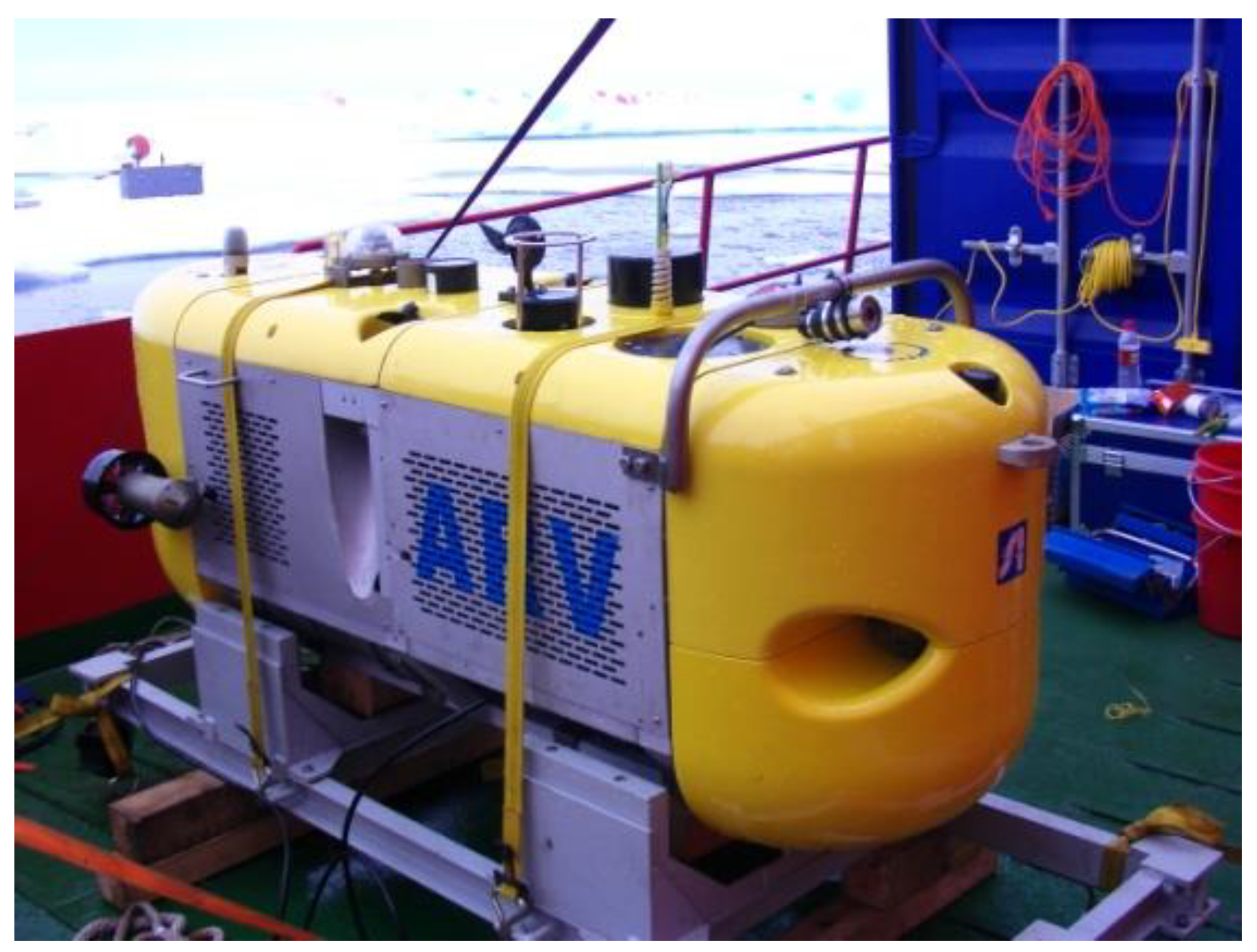
The “Arctic AUV” is a novel autonomous underwater vehicle that can carry a variety of measuring equipment to monitor the marine environment under the Arctic ice. It can not only operate under remote control, but it can also operate autonomously in a pre-programmed way.
Figure 1 is the physical display of the “Arctic AUV”.
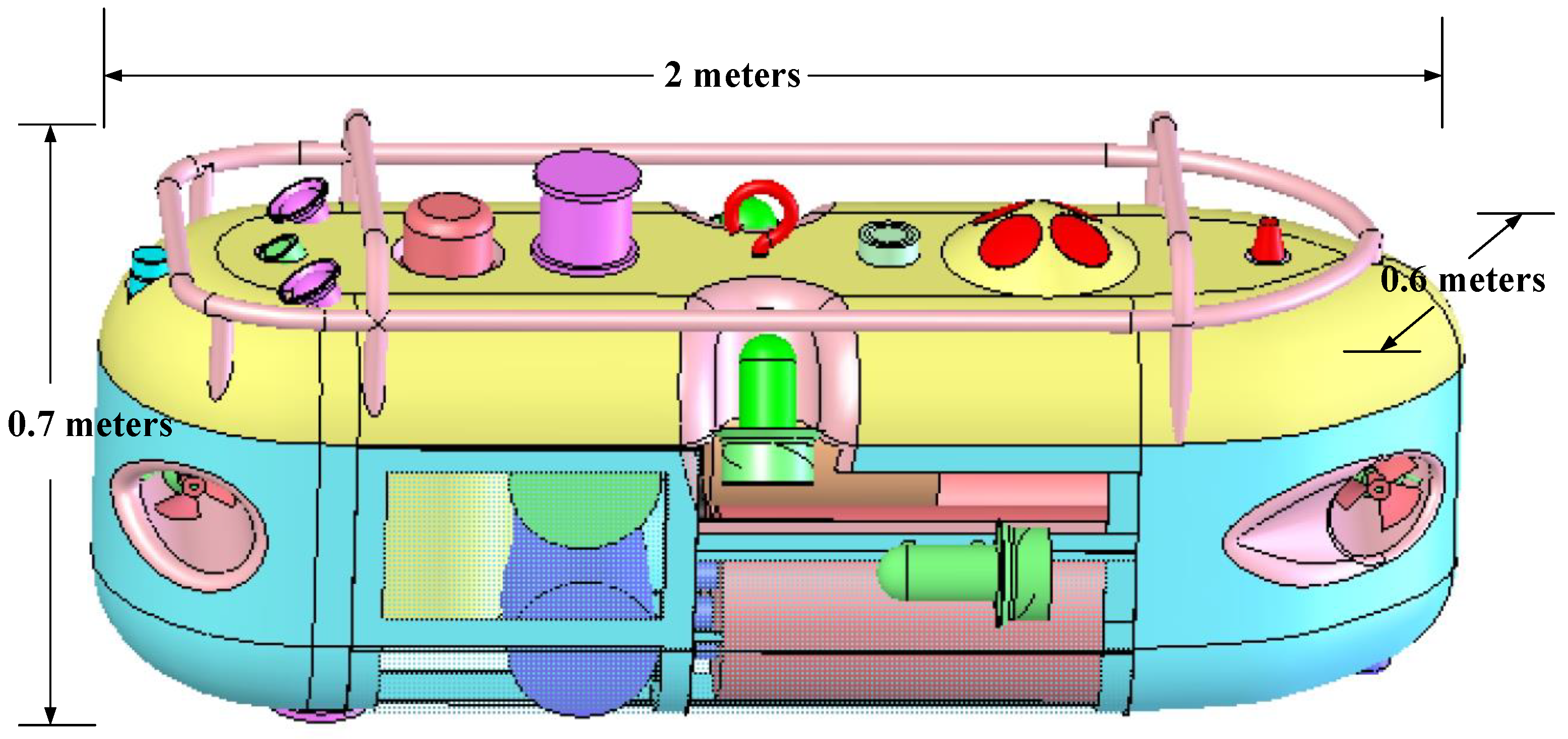
The structure of the “Arctic AUV” is shown in
Figure 2. The “Arctic AUV” has six propellers driven by brushless DC motors. Six thrusters are arranged as follows: two horizontal main thrusters are responsible for the forward and steering motion of the vehicle; two horizontal channel thrusters are responsible for the lateral movement of the vehicle, and two vertical thrusters are responsible for the heave movement of the vehicle. With this thruster arrangement, the AUV system can achieve four degrees of freedom (DOF) motion: forward or backward, side-shift, steering, and heave.
The design size of the “Arctic AUV” is: 2 m (length) × 0.6 m (width) × 0.7 m (height), the weight in the air is 280 kg, the depth of operation is 100 m. “Arctic AUV” has the functions of depth setting, height setting, orientation, and positioning. In the autonomous mode, both directional and fixed-point navigation missions can be carried out. The sensor equipment carried by the Arctic AUV include: a TCM electronic compass, a DVL flow rate measurement sensor, OCTANS inertial navigation sensor, and a depth gauge. The “Arctic AUV” is capable of autonomous navigation under moving sea ice.
The main purpose of the Arctic AUV is to detect the hydrological parameters of the Arctic and the shape of the sea ice in the water. According to the requirements of the detection task, the sensor arrangement of the Arctic AUV is different from that of the traditional underwater vehicles. Many sensors are arranged on the top of the robot, which can easily collect the data under the ice. In addition, in order to prevent the sea ice from colliding with the sensors, an anti-collision device is installed on the top of the robot.
3. The Mathematical Model of “Arctic AUV”
The establishment of the “Arctic AUV” motion model is the premise of studying the motion control of the “Arctic AUV”. The underwater vehicle is a complex nonlinear dynamic system that can also be affected by the external environment. Therefore, not only the dynamic characteristics of the vehicle itself, but also the interference factors of the external environment should be considered when building the motion model of the “Arctic AUV”. In this paper, the mathematical model of the AUV is established, and various interference forces and torques of the AUV are analyzed, which lays a foundation for the design of the controller in the following sections.
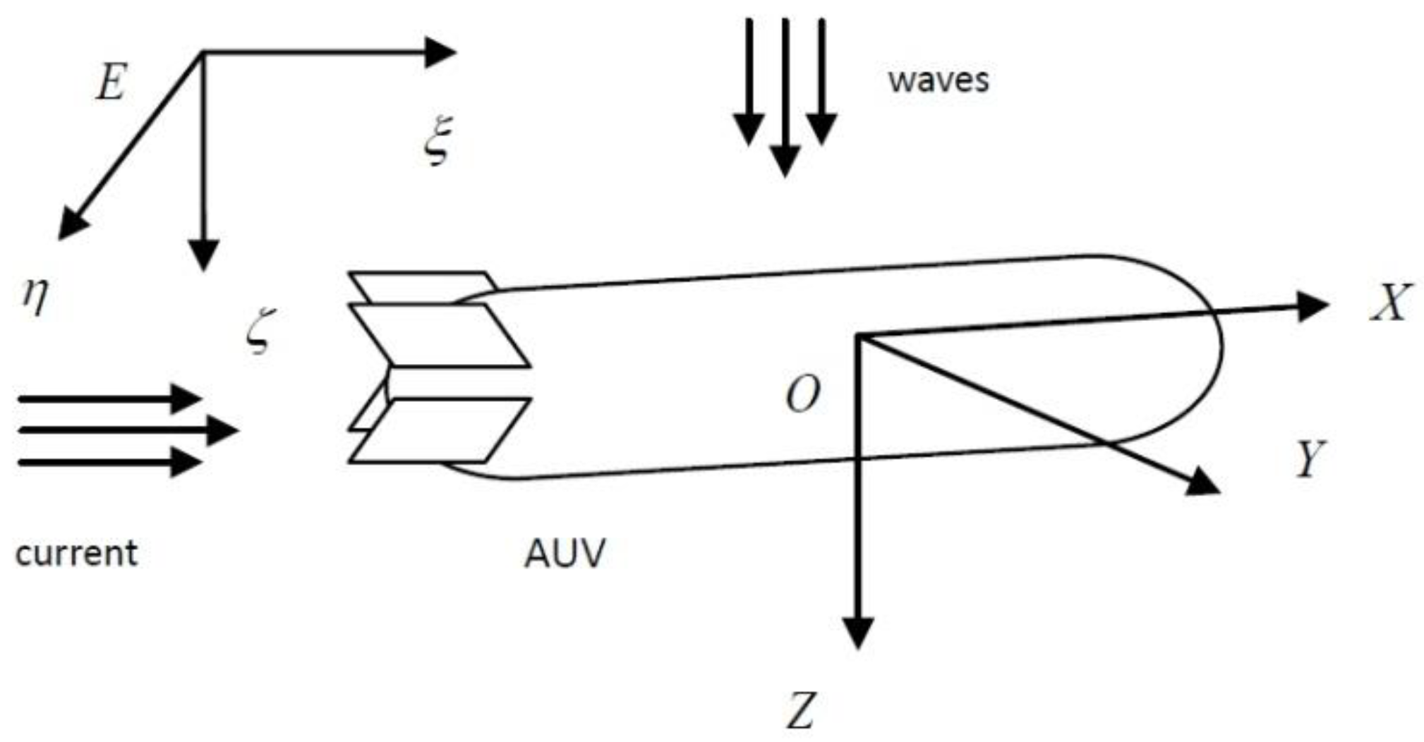
In this paper, an underwater vehicle model based on the Newton–Euler equation is adopted. In order to analyze the kinematics and dynamics of the underwater vehicle, two coordinate systems need to be established: the inertial coordinate system
and the vehicle carrier coordinate system
O-xyz [
28]. The relationship between the two coordinate systems is shown in
Figure 3, and the vehicle carrier coordinate system is usually chosen. The kinetic equation can be established. Since the inertia law can only be applied to the inertial coordinate system, it is necessary to transform the dynamic equation of the vehicle carrier coordinate system into the inertial coordinate system.
According to the Newton–Euler motion equation of the rigid body in the fluid, the 6-DOF dynamics model of the AUV in the vehicle carrier coordinate system can be described as [
3]:
In the equation, mass, and inertia matrix includes rigid body mass and inertia matrix and hydrodynamic additional mass matrix , as .
The Coriolis and centripetal force matrix
of the AUV includes a rigid body centripetal force matrix
and a Coriolis-like force matrix
caused by an additional mass inertial matrix
, namely:
The fluid resistance includes the drag force and lift force of the AUV. At low speed, the lift force is ignored, and the drag force is retained to the quadratic term, then the fluid resistance matrix is:
and
are linear and quadratic resistance coefficients respectively, which can be expressed as:
is the restoring force (moment) vector generated by gravity and buoyancy,
;
is the force (moment) vector generated by the propeller,
.
transforms the linear (angular) velocity vector in the vehicle carrier coordinate system into the corresponding vector in the inertial coordinate system. All coefficients in Equations (4) and (5) are listed in
Table 1.
The roll angle of the AUV is too small to control. The underwater vehicle is symmetrical at about three sections; Coriolis and centripetal force can be ignored at low speed. Assume that gravity is equal to buoyancy, i.e., W = G. Therefore, the dynamic model of the AUV can be simplified as:
In the motion coordinate system, the coordinate of the gravity center of the underwater vehicle is
the coordinate of the buoyancy center is
, So the center of buoyancy is also on the
Oz axis. Here is
The combined force of the gravity and buoyancy of the underwater vehicle only affects its movement in the direction of the heave freedom. Moreover, when the underwater vehicle is completely immersed in water, the buoyancy, which is generated by the water on the underwater vehicle, is greater than the gravity experienced by the underwater vehicle. It can ensure that when the underwater vehicle works underwater, it can rely on positive buoyancy to float on its own, in case of failure.
According to the above simplified formulas, the dynamics model of the AUV in three degrees of freedom directions can be obtained. In the motion coordinate system, the dynamics model of the AUV with a single degree of freedom is:
The horizontal course loop of the AUV can be described by Equation (11). The depth control of the “Arctic AUV” is carried out in the following way: the vertical inclination of the AUV is controlled by a horizontal rudder, and the depth of the AUV is changed by the forward velocity and the longitudinal inclination. At this time, the vertical velocity in the vehicle body coordinate system is very small.
In the form of second order Nomoto model:
is the time constant,
is the steady state gain.
is the delay time. The Laplace transform:
is also the time constant,
is also the steady state gain.
is the delay time. The Laplace transform:
The time constant and the steady state gain are the main parameters that affect the transient and steady state characteristics of the control system. In the process of designing the control system, these two parameters have a decisive influence on the controller parameters. These two parameters are very important to the design of the control system and the online adjustment of the controller parameters.
4. “Arctic AUV” System Identification
In the previous section, the dynamic model of the underwater vehicle was established and simplified through theoretical analysis, but there are still some parameters that need to be determined in the dynamic model. The determination of these parameters can be accomplished by parameter identification of the dynamic model of the underwater vehicle. The higher the accuracy of the identified parameters, the more accurate the dynamic model will describe the underwater vehicle’s motion state.
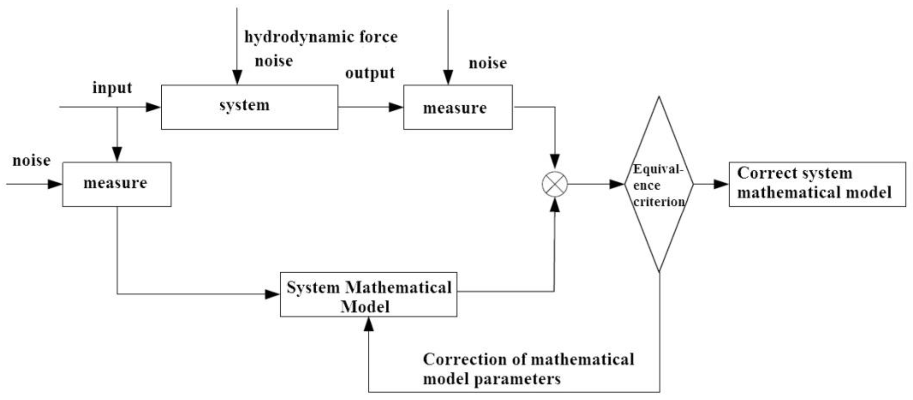
The purpose of system identification is to estimate the unknown parameters of the model under a certain error criterion, based on the measurement information provided by the process. The principle is shown in
Figure 4.
In order to obtain the estimated value
of model parameters
, generally, the method of gradual approximation is adopted. At time
k, the output of the model at that time is calculated according to the estimated parameters at the previous time, that is, the process output forecast value:
Calculate the forecast error:
and is measurable, bring into the identification algorithm, under a certain criterion condition, calculate the estimated value of the model at time , and iterate continuously with the new model parameters until the criterion function converges to a predetermined minimum value.
In order to improve the accuracy of the parameter estimation of the dynamic model of the underwater vehicle and enable the identification algorithm to perform real-time calculations, this paper proposes a total least squares algorithm fusion algorithm based on the multi-sensor fusion data fusion, and on this basis, through theoretical derivation multi-sensor fusion based online identification algorithm of underwater vehicle dynamics model parameters.
The model structure adopted by the least square method is:
where
and
represent the output and input of the process,
is an uncorrelated random noise sequence with a mean value of 0.
The augmented least squares method tries to identify the noise model:
Since noise is unknowable, this paper uses the corresponding estimator instead:
In this way, an augmented least squares recursive algorithm with forgetting factor
can be written:
where,
is called the covariance matrix and
is the constant value forgetting factor. When
, it is the general least square method (LS). The algorithm has good convergence properties.
In the multi-sensor system of an underwater vehicle, the to-be-identified model of a single sensor can be written as follows:
where,
,
in the upper right corner is the measurement value of the
sensor among the
N sensors, make
,
, and:
Then the solution in the sense of augmented least squares is:
Make
,
, then the multi-sensor augmented least squares centralized fusion can be written as:
5. Control Scheme Design of the “Arctic AUV”
The previous article analyzes and derives the system identification. In this section, the adaptive control scheme of the “Arctic AUV” is designed from the perspective of engineering application. Using the hierarchical idea, the controller is divided into three layers: the coordination and management layer, the adaptive layer, and the control layer. The coordination and management layer monitor the status of the system at all times, performs fault diagnosis procedures, and immediately makes adjustment strategies in the event of instability or some institutional failures; the adaptive layer implements the identification procedures, filters the measurement data, and determines the validity of the identification results; the control layer is responsible for the solution of the control law. The system structure is shown in
Figure 5.
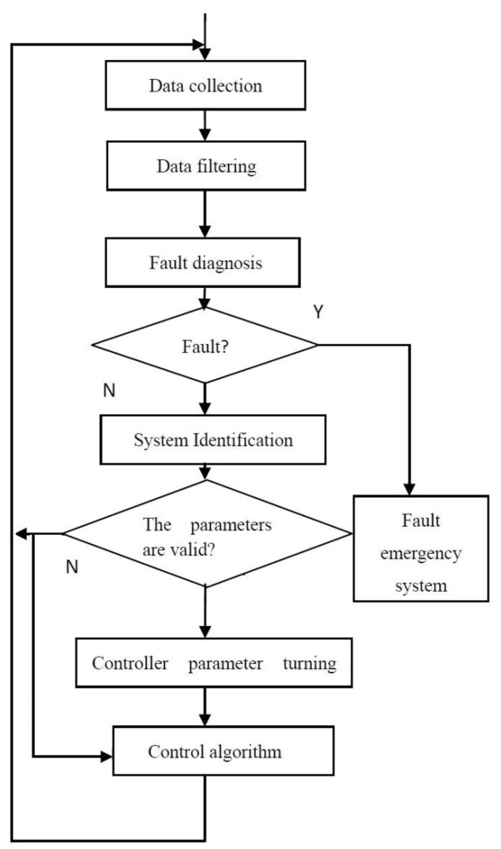
The operation process of the control system is shown in
Figure 6. The data measured by the sensor is first removed and filtered to remove the sensor outliers and high-frequency environmental interference; the fault diagnosis program judges whether the system is faulty based on the measurement data and historical data, and if there is a fault, it will go to the fault emergency system. The system identification procedure recursively identifies the model parameters of the system, judges the effectiveness of the identification results according to the discrimination criteria, and uses the obtained model parameters to tune the controller parameters. If the identification results are invalid, the system will execute the control law that was tuned last time.
6. Self-Tuning Control Algorithm of “Arctic AUV”
“Arctic AUV” adopts self-tuning PID control to solve the problem of time-varying parameters. Self-tuning PID control combines PID control and parameter identification. The adjustment of PID parameters is set by the parameters obtained by system identification and pre-designed performance indicators.
This paper obtains the model parameters of the system through the method of system identification and combines the identification parameters and the tuning of PID parameters to form a self-tuning PID control. First, the PD control rate is given:
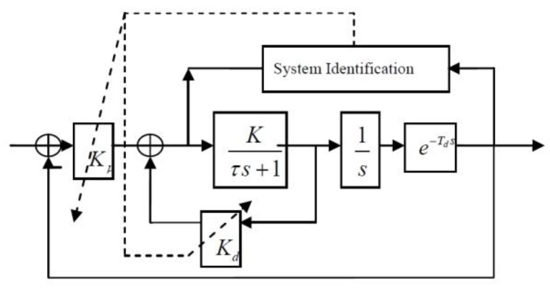
The control system structure is shown in
Figure 7.
The differential control term here does not use error differentiation but speed feedback. The advantage of this is that the closed-loop system will reduce a zero point and the transient performance is good. The closed-loop system equation is:
The undamped natural frequency is denoted by
, and the damping coefficient is denoted by
.
It can be deduced from this:
It can be seen that
Kp and
are related to the time constant
of the system, the steady-state gain
K, and the desired response characteristics. The controller can be designed according to the expected performance indicators and the characteristic parameters of the underwater vehicle, but the
and
K of the “Arctic AUV” is changing during the navigation process. The identification method is as follows:
Using the identified and K parameters, the PID controller can be corrected in real time, so that the output response of the system always conforms to the designed response characteristics.
Due to the existence of environmental interference, the underwater vehicle will have steady-state errors during navigation. In order to eliminate the steady-state error, it can be compensated by adding an integral link. Take the control law as:
The integral coefficient adopts the anti-saturation method, and
is the error band that needs to be adjusted. Here
parameter is selected as:
In order to improve the robustness of the system, a robust compensation term is added to the control law:
The magnitude of the robust compensation term affects the robustness of the system. If a large, fixed value is selected to ensure the stability of the system under the maximum interference, the output of the controller will be very large or even saturated. Here, it is automatically adjusted according to the value of the PD controller.
is the design parameter:
The purpose of the robust compensation item is to produce a control quantity when is greater than zero, so that is generated.
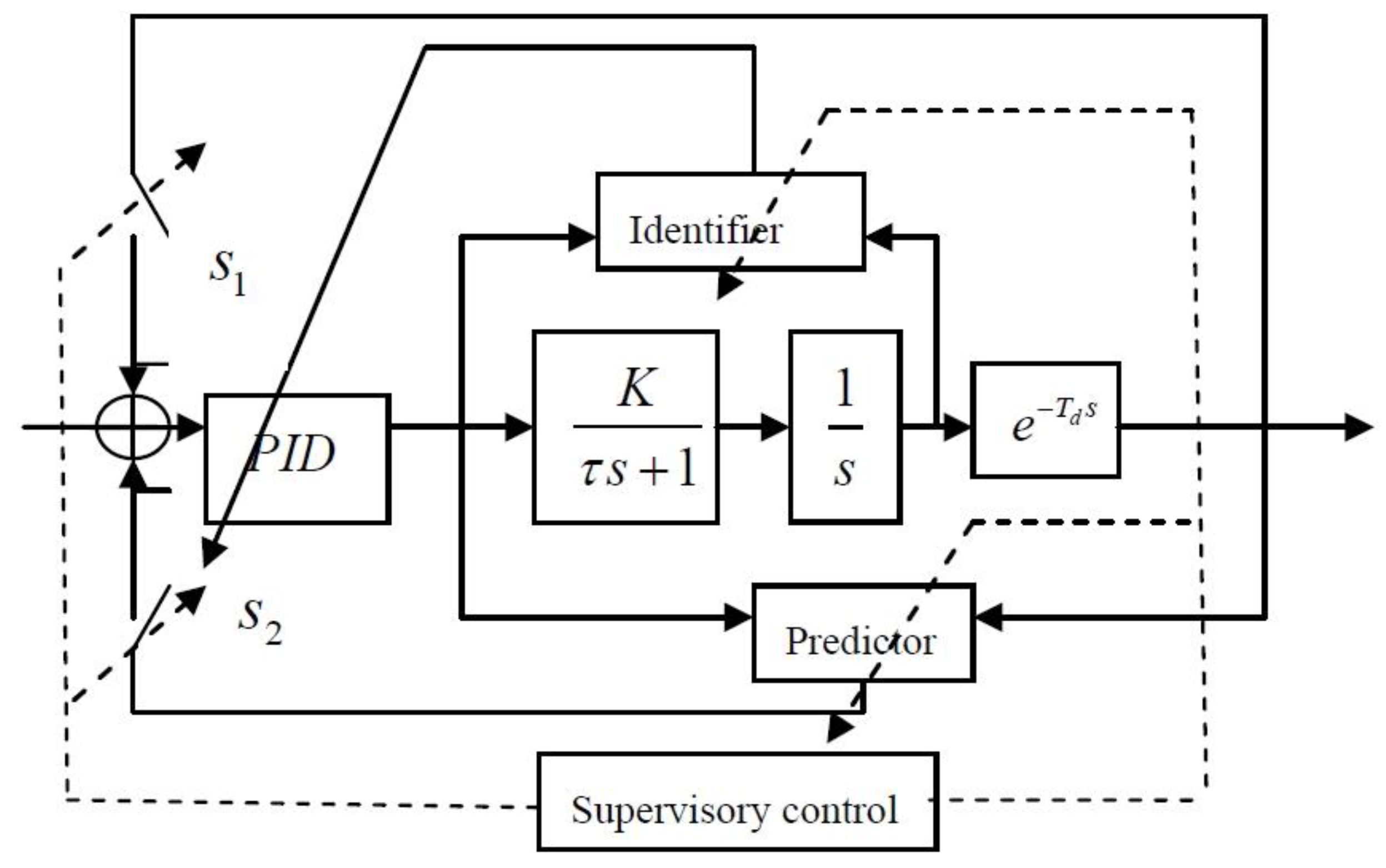
In addition, “Arctic AUV” also uses predictive PID controller structure diagram, shown in
Figure 8. The controller includes: PID control module, recognizer, predictor, and supervisory controller. The role of the supervisory controller is to judge the effectiveness of system identification and prediction, and only run the response algorithm when it is judged to be effective. The system operation process is that the PID control method is adopted after the system is started. The identifier and the predictor work at the same time. According to the parameter validity criterion, when the predictor output is valid, the predictive PID control is adopted, and when the identifier output is valid, the self-tuning PID control is adopted.
7. Experiments
7.1. System Identification of “Arctic AUV”
This section uses the mathematical models and system identification methods of the previous chapters to identify the parameters of the “Arctic AUV”. The identification experiment consists of two parts: offline identification and online identification. The offline identification method is to record the operation data of the “Arctic AUV” through the pool experiment, and then analyze and identify the data to obtain the model parameters. Offline identification is mainly to obtain the model parameters of the “Arctic AUV” and use these parameters to analyze the system and design the controller. The method of online identification is to embed the identification algorithm into the “Arctic AUV” controller to identify the model parameters of the system in real time. Online identification is mainly used for adaptive control.
The focus of this paper is the heading loop and depth loop of the “Arctic AUV”. The following are the experiments on the heading loop and depth loop of the “Arctic AUV” from two aspects of offline and online identification.
7.1.1. Offline Identification of “Arctic AUV”
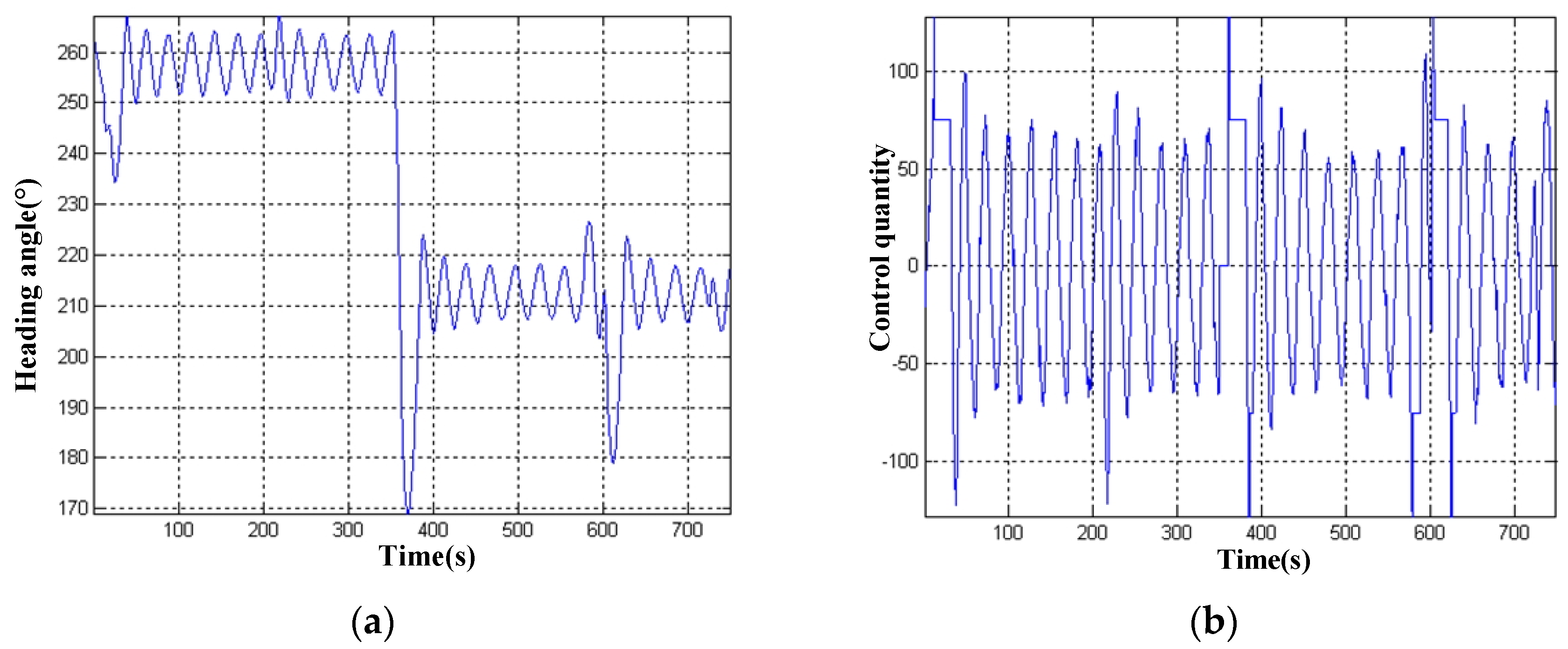
Parameter Identification of Heading Loop
During the experiment, the heading loop adopts the PID controller, and the parameters are
10,
20,
0.
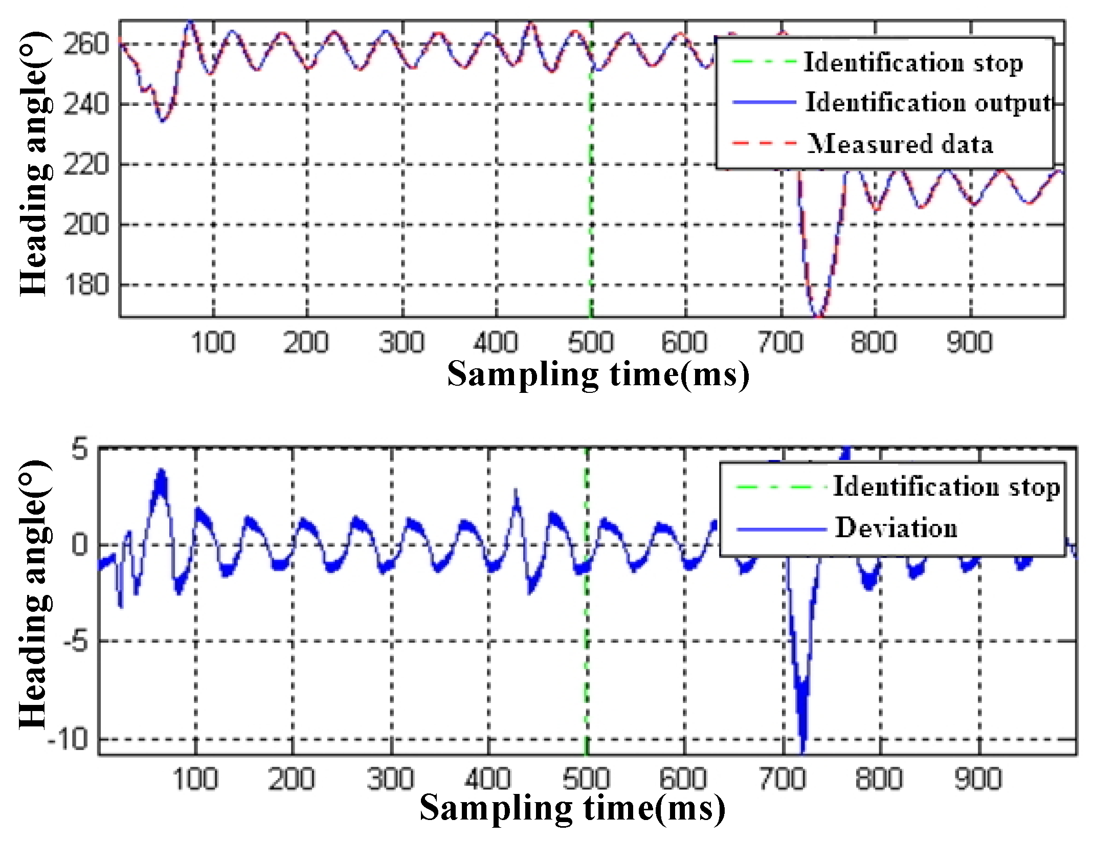
Figure 9 shows the heading angle and control curve recorded by the experiment.
Determination of delay time d: the delay time of the system is the minimum of the variance of the residual variance.
Table 2 shows the variance of the corresponding residuals when d is taken at different values.
It can be seen from
Table 2 and
Table 3 that when the delay time parameter is d = 6, the variance of the residual error of identification is the minimum. As the sampling time is 0.5 s, the delay time of the heading angle loop is 3 s. The identification results obtained at this time are:
−1.8615,
0.8615,
0.0020,
3.3531,
0.0286. The mathematical model of the heading loop is:
Figure 10 shows the comparison curve between the identified output data and the actual data.
7.1.2. Parameter Identification of Depth Loop
During the experiment, the depth loop adopts PID controller, and the parameters are
60,
40,
0.
Figure 11 shows the depth and control curve of the experimental record.
Due to the effect of positive buoyancy, the model of the depth loop of the underwater vehicle is slightly different from that of the heading loop:
is the thruster control quantity,
is the residual buoyancy force,
is the resultant force in the vertical plane,
. The resultant force
should be calculated before parameter identification. The key is to calculate the residual buoyancy of the underwater vehicle. The adopted method is to take the average value of the output data of the control quantity in the stability section of the depth closed-loop control to analyze the residual buoyancy of the vehicle.
Figure 12 shows the output curve of depth control quantity obtained from the pool experiment.
As can be seen from the depth control quantity, the control quantity has a direct current component to overcome the buoyancy force on the vehicle carrier when it is stable. The averaged data in the stationary section is U = 55.062, which is the same unit as the control quantity
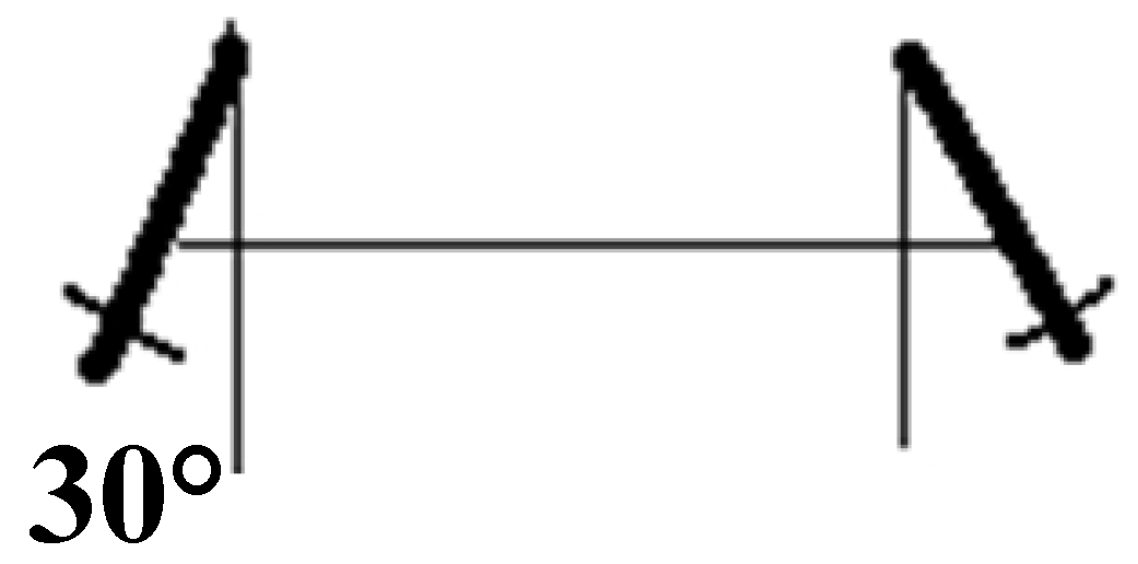
in the vertical plane. The arrangement of the vertical propeller is shown in
Figure 13.
U = 55.062 corresponds to a propeller thrust of 0.32 kg. The combined thrust of the two propellers is 0.27 kg. The “Arctic AUV” has a positive buoyancy of 2.7 N.
Applying the
Z transformation to
(sampling period is
T):
Writing it as a discrete time series:
Writing it in general terms for a second order system:
Determination of delay time d: the delay time of the system is the minimum of the variance of the residual error.
Table 4 shows the variance of the corresponding residuals when d is taken at different values.
It can be seen from
Table 4 and
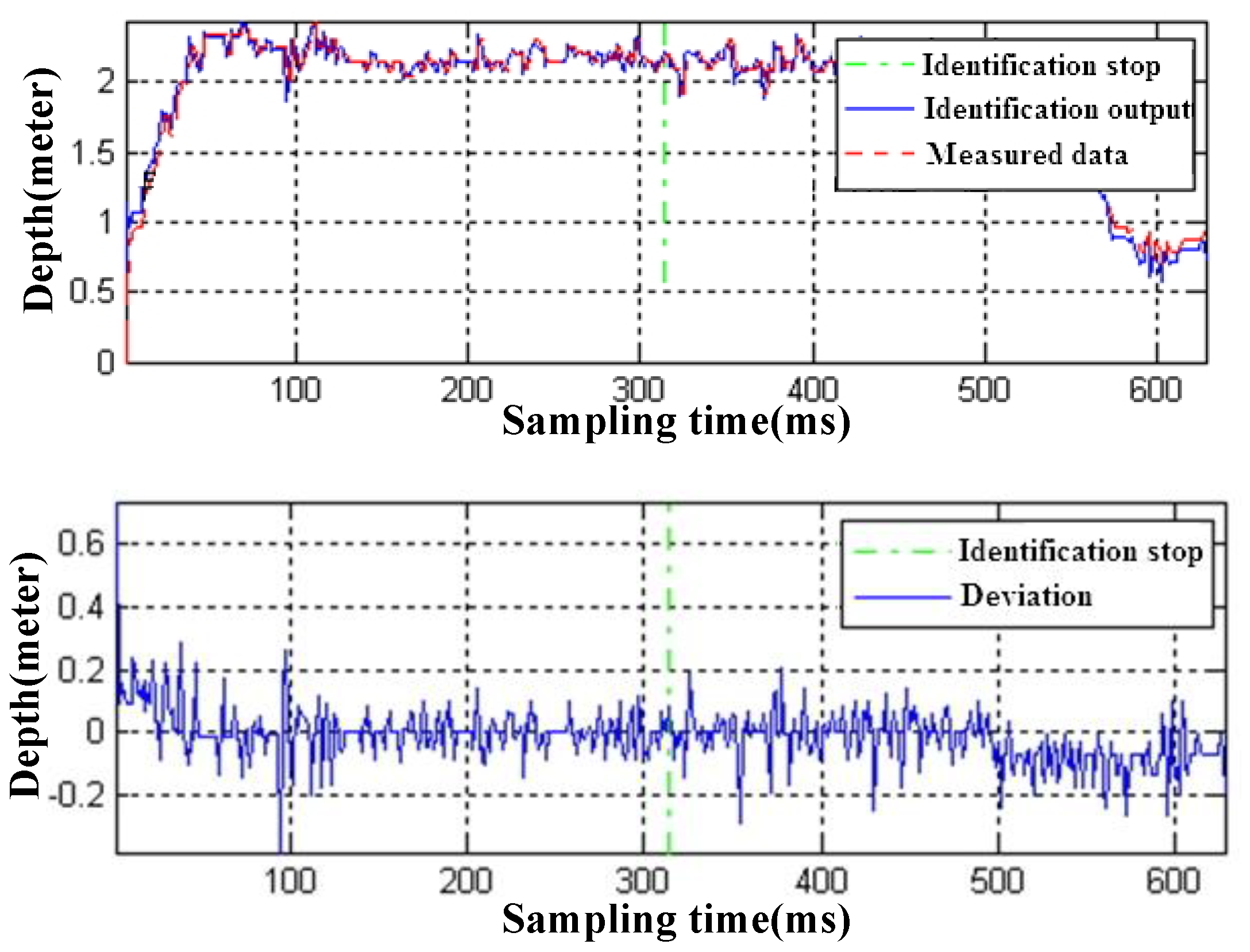
Table 5 that when the delay time parameter of the identification model is d = 0, the residual variance of identification is the minimum. Since the sampling time is 0.5 s, the delay time of the depth loop is 0 s. The identification result is as follows:
−1.3651,
0.3653,
0.0013,
0.4965,
0.0042.
The mathematical model of the depth loop is:
Figure 14 shows the comparison curve between the identified output data and the actual data.
7.1.3. Online Identification of “Arctic AUV”
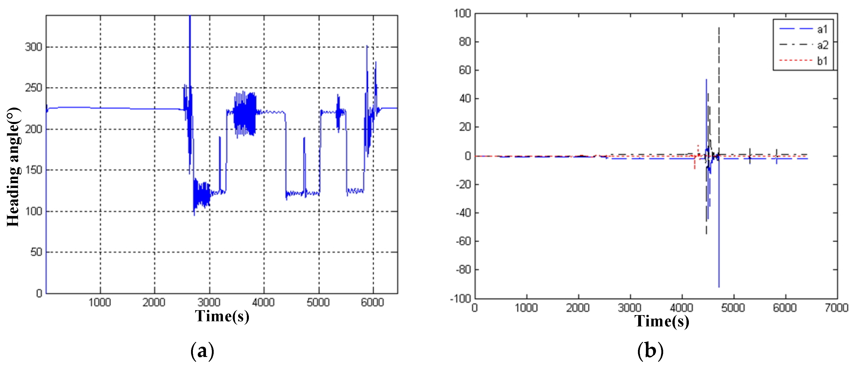
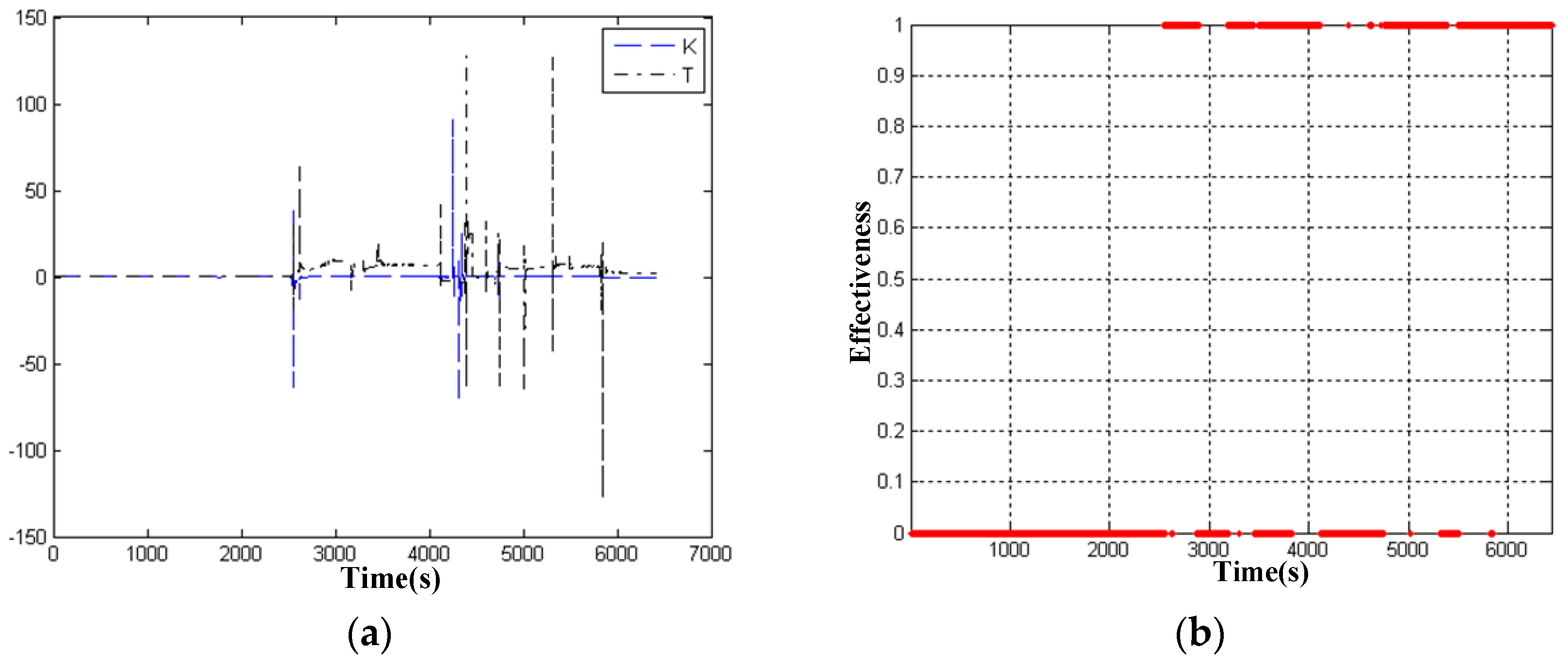
The online identification parameters are mainly used to adjust the coefficient of the controller, so the effectiveness of the parameters is very important. In this section, the validity of the online identification method is verified by experiments. Water flow interference is added during the experiment. A covariance resetting method is used to avoid covariance matrix overflow or singularity in the process of identification. The results of identification experiment are shown in
Figure 15 and
Figure 16.
It can be seen from the identification curve that in the first half of the period, because the AUV did not go into the water, the parameters identified at this time were wrong. After the AUV entered the water, the identification parameters converged most of the time, however in the transition stage, or when the disturbance was relatively large, the identification parameters were wrong. It is necessary to judge the validity of the parameters to determine whether the parameters identified can be used for AUV control in practical engineering applications.
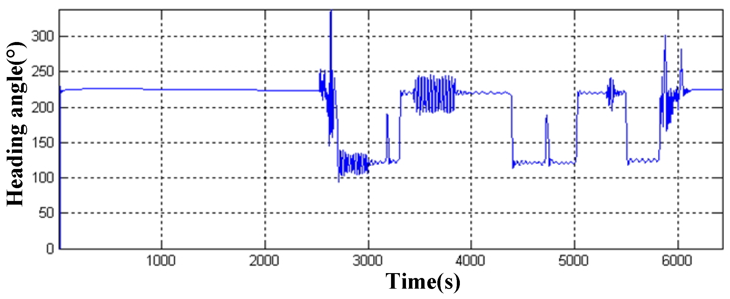
7.2. Self-Tuning PID Control Experiment
The self-tuning PID control is applied to the heading control loop of “Arctic AUV”. Since the adaptive control algorithm uses online identification to adjust the parameters of the controller, according to the analysis in the previous section, when the identification parameters are not accurate, the controller needs to switch to the PID controller with fixed parameters. Here, the parameters of the PID controller are
p = 15, D = 0, and I = 0. Target heading angles were set at 123° and 223°.
Figure 17 shows the experimental response curve.
At first, the system identification could not converge to the true value, and the heading angle oscillation was serious. However, when the true value of the parameters are identified, the parameters of the controller are adjusted according to the designed indexes and the control effect reaches the expected design index. In order to verify the robustness of the system, water flow interference and pull rope interference are added to the system. When the identification has an error, the system automatically switches to the fixed parameter PID controller, and then automatically switches to the adaptive controller after the identification convergence. The validity of the self-tuning PID controller is verified by experiments.
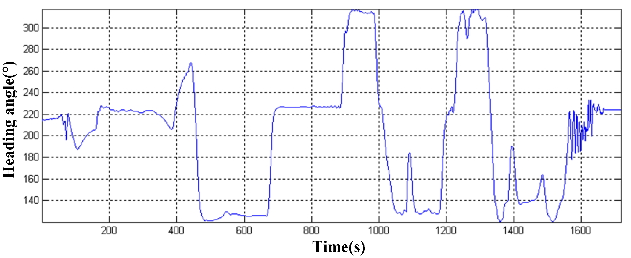
The above analysis of the “Arctic AUV” system identification deduced that the system has a delay of 3 s, the use of fixed parameters of the PID control effect is not ideal, and the adaptive predictive PID control can be applied to the heading control loop. The control cycle is 0.5 s, therefore the predicted step size is 6 steps. Target heading angles are 223°, 123° and 313°, with flow interference, and sailing speed of 1 knot. The experimental results are shown in
Figure 18.
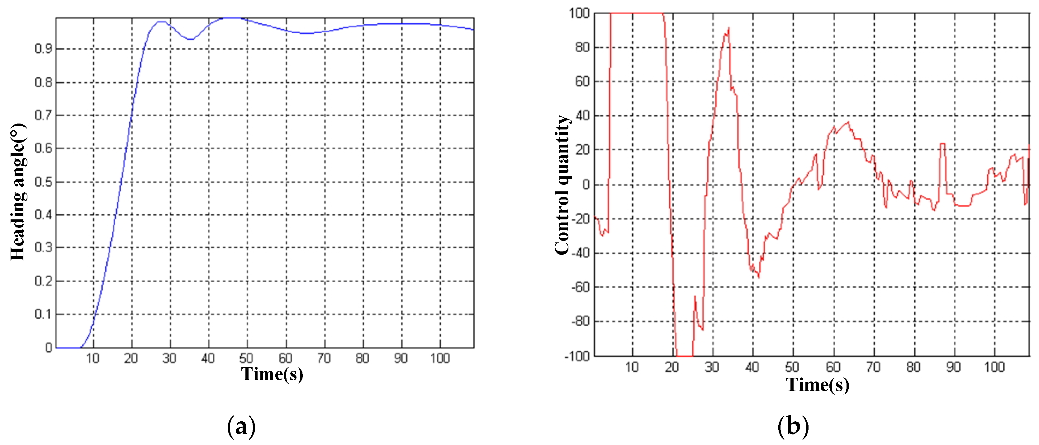
In order to demonstrate the effectiveness of the algorithm, the step response of the adaptive predictive PID control is compared with the response of the traditional PID control under the same parameters.
Figure 19 shows the response curve with ordinary PID control.
Figure 20 shows the response curve of sampling prediction PID control.
It can be seen from the curve that the adaptive predictive PID control effect is obviously better than the fixed parameter PID control. Of course, for the delay problem of the underwater vehicle, we should first start from the nature of the problem and find a method to reduce the delay. When the delay problem cannot be fundamentally solved, the adaptive predictive PID control method will be considered.
The experimental results show that the mathematical model established in this paper can reflect the motion state of the “Arctic AUV” more truly, so it is of great significance to study the manoeuvrability and adaptive control of the “Arctic AUV”. Both the self-tuning PID control and adaptive sliding mode control have good control effects, fast responses, no overshoots or steady state errors, a smooth change of control quantity, and no obvious chattering phenomenon, etc. Only in the case of strong interference will the output of the system identifier be severely affected. The experiment verifies the robustness of the control algorithm in this case.
8. Conclusions
This paper takes the “Arctic AUV” control in a complex ocean environment as the starting point for research, then a large number of theoretical derivation and experimental verification are carried out from two aspects of system parameter identification and motion control, and the mathematical model of the “Arctic AUV” is established. The relationship between the mathematical model of system identification and the physical variable of the vehicle is derived. The influence of the complex ocean environment on the control of the underwater vehicle is analyzed, and the hybrid scheme of self-correcting PID control and predictive control is applied to the control of the “Arctic AUV”. The heading loop and depth loop of the “Arctic AUV” are identified, and the validity of the model is verified by experiments.


