Precise Locating Control for a Polar Crane Based on Sliding Mode Active Disturbance Rejection Control and Quadratic Programming Algorithm

Abstract

A polar crane is a large-scale special lifting equipment operated in a nuclear power plant. To address the precise locating control problem of a polar crane with the center of gravity shifting, with cross-coupling, and with external disturbance, an effective control scheme is proposed in this paper. Firstly, a nonholonomic constraint dynamic model of the polar crane is established according to the Lagrange–Rouse equation. Then, an expansion state observer (ESO) of the active disturbance rejection control (ADRC) method is applied to estimate and compensate the cross-coupling disturbance in real-time. To improve the robustness and convergence speed of the control system, the nonsingular terminal sliding mode (NTSM) control method is incorporated with ADRC and the stability of the controller is proven by the Lyapunov function approach. Furthermore, to solve the problem of redundant actuation and to reduce trajectory deviation of the bridge truck, the contact forces of the horizontal guide device are introduced into the quadratic programming (QP) optimization algorithm. Finally, the effectiveness and superiority of the proposed control scheme are illustrated by simulation results.

1. Introduction

A polar crane is a large-scale special lifting equipment operated at the top of a containment vessel; it is mainly used for heavy equipment lifting and fuel replacing. Taking the lifting process of reactor pressure vessel upper heads as an example, the hook block needs to be slowly lowered and accurately aligned with the center of the reactor pressure vessel, which places a high demand for precision lifting on the polar crane.

Reliable manufacturing processes and reasonable structural design methods are the basis for precise lifting of a polar crane. Literature [1] took the physical structure of the rope-sheave system of the polar crane into account and proposed a systematic method for analyzing the dynamics of the system based on the virtual power principle. Literature [2] presented a quasi-static method to analyze the equilibrium path and trajectory deflections for the load of the polar crane, which is of great significance for improving the structural layout of the lifting system. Literature [3] proposed a static balanced approach to analyzing the straightness deviation of the hook block during the lifting process. Literature [4] analyzed the influence of bridge deformation on the locating accuracy under different working conditions by the finite element method. Literature [5] presented an effective control method for the welding deformation of corbel by improving the welding process and welding sequence. Literature [6] analyzed the rigid-flexible coupling model of a polar crane based on the ANSYS and ADAMS co-simulation analysis method. The results obtained have important reference values in analyzing the influence of structural flexibility on locating accuracy.

Related studies did not consider the impact of the operation process on lifting accuracy. In the field of traditional hoisting machinery, a series of control technologies is relatively mature and provides an important reference for the polar crane. In the aspect of swing suppression control, Literature [7] aimed for a double pendulum structure of overhead cranes and proposed a trajectory tracking and swing suppression control method based on sliding mode control theory. Literature [8] proposed a multivariable generalized predictive control method for an overhead crane based on the particle swarm optimization algorithm and achieved good control performance. Literature [9] designed a linear quadratic regulator based on Takagi–Sugeno fuzzy modeling and particle swarm optimization algorithm for anti-swing and positioning control of the overhead crane. In terms of crane trajectory planning, aimed at the problem of payload residual swing caused by inertial force, Literature [10] designed the acceleration curve of the trolley based on the energy control method. Literature [11] proposed an energy optimal model of the overhead crane according to energy consumption, operation time, and safety. To deal with the problem of parameter uncertainty in the trajectory planning, Literature [12] proposed an uncertain estimation and optimization scheme which provides guidance for uncertain analysis and online controller design of overhead cranes. Literature [13] proposed a new control system based on the state feedback control method to deliver high-performance trajectory tracking with minimum load swings in high-speed motions. In the field of the offshore ship-mounted crane, Literature [14] designed a neural network-based adaptive controller to solve the payload swing caused by sea waves. Literature [15] proposed a novel event-triggered fuzzy robust fault-tolerant control approach to overcome actuator fault and external disturbance of offshore ship-mounted crane. Literature [16] designed an observer-based nonlinear feedback control to achieve simultaneous accurate jib/trolley positioning and fast payload swing suppression against complex unknown external disturbances.

A polar crane is a nonlinear control system with multiple inputs, multiple outputs, and strong coupling. Moreover, due to the movement of the trolley, a polar crane is often in a state of center of gravity shift during rotation. As an effective nonlinear control method, active disturbance rejection control (ADRC) has the advantages of simple, feasible, and strong robustness, and for the coupling system, the cross-coupling disturbance can be estimated and compensated by the ESO. Therefore, compared with the traditional decoupling control method, ADRC has significant advantages [17,18,19] and can be an important method to solve the control problem of the polar crane.

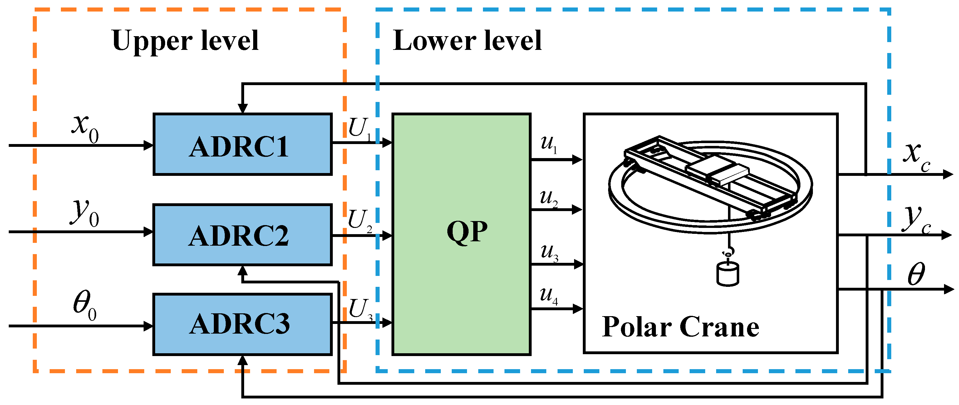
As stated previously, most studies in the field of precise lifting of a polar crane have only focused on the lifting mechanism design and analysis, but the problem of location deviation during crane operation has been ignored. To address this problem, a novel locating control scheme for the polar crane is proposed in this paper. The main contributions of this paper are summarized as follows:

(1)

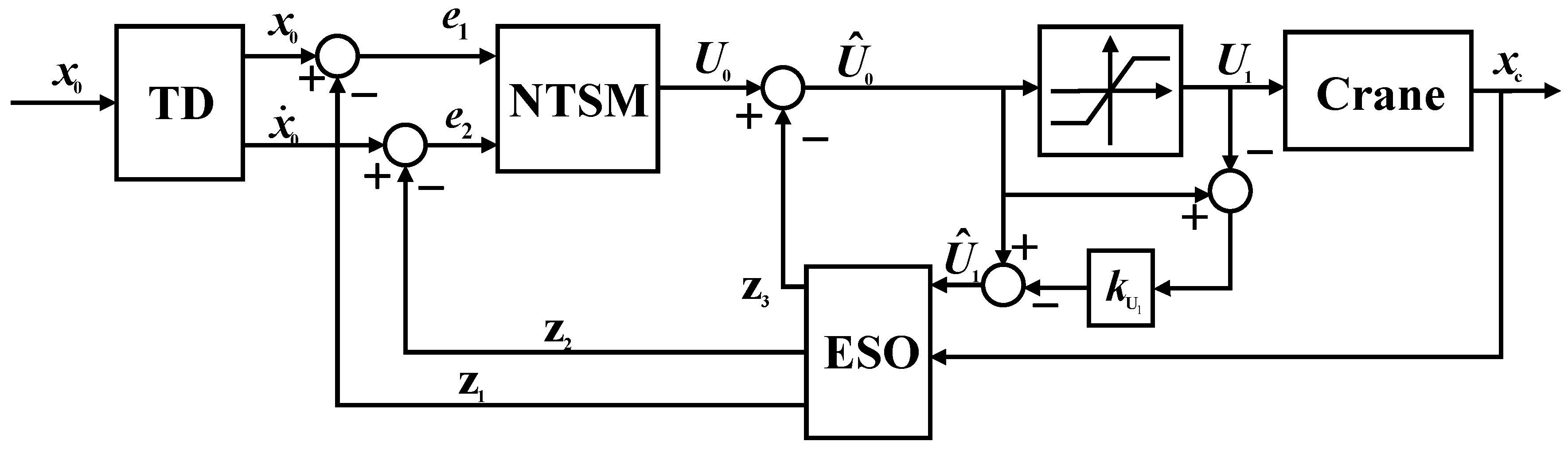
An nonsingular terminal sliding mode (NTSM)-ADRC-based decoupling method is first proposed to effectively address the cross-coupling disturbance for the polar crane system and to greatly improve the robustness and adaptability of the crane system.

(2)

To properly address the problem of redundant actuation, a quadratic programming (QP) optimization model is designed, in which the contact force of the horizontal guide device is introduced to reduce the trajectory deviation of the bridge truck.

(3)

The proposed NTSM-ADRC-QP control scheme has good performance in locating control under the conditions of center of gravity shift and external disturbance.

The paper is organized as follows: The nonholonomic constraint dynamic model of the polar crane and model validation are introduced in Section 2. Section 3 illustrates the overall structure of the NTSM-ADRC-based decoupling control method, the stability analysis, and the quadratic programming algorithm for the polar crane. Numerical simulations and analyses are provided in Section 4 for the proposed control scheme. Finally, Section 5 concludes the main works of this paper.

2. Crane Description, Modeling, and Simulation

A polar crane is installed on the top of the containment vessel. As shown in Figure 1, the main structures include a crane bridge, a bridge truck, a trolley, a lifting mechanism, a horizontal guide device, and an electrical system.

The bridge truck is used to drive the crane rotating on the rail, and the trolley is installed on the crane bridge; thus, it can move on the crane bridge. Based on the cooperative movement between the trolley and the bridge truck, the lifting mechanism can cover all areas of the reactor building. In addition, horizontal guide devices are installed to ensure the crane operates safely.

2.1. Dynamic Model of the Polar Crane

In Figure 2, a graphical representation of the polar crane is shown. It could be seen that $\left\{X,O,Y\right\}$ is a global coordinate frame attached to the center of the rail, $\left\{x,P_c,y\right\}$ is a local coordinate frame attached to the polar crane, $P_c$ is the geometric center of the crane, and $P_G$ is the center of mass of the crane.

Under the condition of planer movement, the configuration of the polar crane can be described by seven generalized coordinates. Among them, three variables describe the position and orientation of the crane, and four variables describe the motion states of the driving wheels:

$$\mathit{q}={\left[x_c,y_c,\theta ,{\phi }_1,{\phi }_2,{\phi }_3,{\phi }_4\right]}^T,$$

where $\left(x_c,y_c\right)$ are the coordinates of the geometric center $P_c$ in the global coordinate frame; $\theta$ is the rotation angle of the polar crane; and ${\phi }_1$, ${\phi }_2$, ${\phi }_3$, and ${\phi }_4$ are the angular displacements of the driving wheels installed in the bridge truck.

Moreover, the corresponding system parameters are illustrated in

Table 1. Structure parameters of the polar crane.

Symbol	Description	Unit	Symbol	Description	Unit
$L_1$	Length of the crane bridge	$\mathrm{m}$	$m$	Mass of the trolley	$\mathrm{kg}$
$L_2$	Width of the crane bridge	$\mathrm{m}$	$r$	Radius of the driving wheel	$\mathrm{m}$
$l$	Length of the outrigger	$\mathrm{m}$	${\delta }_1$	Angle between wheel axle and x axis	$\mathrm{deg}$
$R$	Radius of the rail	$\mathrm{m}$	${\delta }_2$	Angle between outrigger and x axis	$\mathrm{deg}$
$M$	Mass of the crane bridge	$\mathrm{kg}$	$d$	Distance between the trolley and $P_c$	$\mathrm{m}$

.

According to Figure 2, the relationship between the geometric center $P_c$ and the center of mass $P_G$ can be depicted as follows:

$$\begin{array}{l}{x}_g=x_c-\frac{md}{M+m}\cos \theta \\ y_g=y_c-\frac{md}{M+m}\sin \theta \end{array},$$

(1)

where $\left(x_g,y_g\right)$ are the coordinates of the center of mass $P_G$ in the global coordinate frame.

Assuming a pure rolling condition for the driving wheels, the following constraint equations can be derived:

$$\{\begin{array}{c}-{\dot{x}}_c\sin (\theta +{\delta }_1)+{\dot{y}}_c\cos (\theta +{\delta }_1)+R\dot{\theta }=r{\dot{\phi }}_1\\ {\dot{x}}_c\sin (\theta -{\delta }_1)-{\dot{y}}_c\cos (\theta -{\delta }_1)+R\dot{\theta }=r{\dot{\phi }}_2\\ {\dot{x}}_c\sin (\theta +{\delta }_1)-{\dot{y}}_c\cos (\theta +{\delta }_1)+R\dot{\theta }=r{\dot{\phi }}_3\\ -{\dot{x}}_c\sin (\theta -{\delta }_1)+{\dot{y}}_c\cos (\theta -{\delta }_1)+R\dot{\theta }=r{\dot{\phi }}_4\end{array},$$

(2)

The matrix form of the constraints in Equation (2) can be rewritten as follows:

$$\mathit{A}\left(\mathit{q}\right)\dot{\mathit{q}}=\mathbf{0},$$

(3)

where

$$\mathit{A}\left(\mathit{q}\right)=\left[\begin{array}{ccccccc}-\sin \left(\theta +{\delta }_1\right)& \cos \left(\theta +{\delta }_1\right)& R& -r& 0& 0& 0\\ \sin \left(\theta -{\delta }_1\right)& -\cos \left(\theta -{\delta }_1\right)& R& 0& -r& 0& 0\\ \sin \left(\theta +{\delta }_1\right)& -\cos \left(\theta +{\delta }_1\right)& R& 0& 0& -r& 0\\ -\sin \left(\theta -{\delta }_1\right)& \cos \left(\theta -{\delta }_1\right)& R& 0& 0& 0& -r\end{array}\right],$$

(4)

The Lagrange–Rouse equation is used to derive the dynamic equations of the polar crane, since the planer movement of the crane, the total kinetic energy $L$, can be written as follows:

$$L=\frac{1}{2}\left(M+m\right)\left({\dot{x}}_g{}^2+{\dot{y}}_g{}^2\right)+\frac{1}{2}{J}_d{\dot{\theta }}^2+{\displaystyle \sum _{i=1}^4\frac{1}{2}}{J}_{\omega }{\dot{\phi }}_i^2,$$

(5)

where $J_{\omega }$ is the rotary inertia of the driving wheel and $J_d$ is the equivalent rotary inertia of the crane bridge and trolley around the center of mass $P_G$. Note that $J_d$ will change in response to the variation of the parameter $d$.

The Lagrange–Rouse equation of motion for the polar crane system is governed by the following [20]:

$$\frac{\mathrm{d}}{\mathrm{dt}}\left(\frac{\partial L}{\partial {\dot{q}}_j}\right)-\frac{\partial L}{\partial q_j}=F_j+{\displaystyle \sum _{k=1}^4{\lambda }_k{B}_{kj}},j=1,2\dots 7,$$

(6)

where $q_j$ is the element of $\mathit{q}$, $F_j$ is the generalized force, ${\lambda }_k$ is the Lagrange multiplier, and $B_{kj}$ is the element of $\mathit{A}\left(\mathit{q}\right)$.

Substituting the derivative of Equations (1) and (5) into Equation (6), the dynamic equations can be expressed by the generalized coordinates:

$$\begin{array}{l}\left(M+m\right){\ddot{x}}_c+md\ddot{\theta }\sin \theta +md{\dot{\theta }}^2\cos \theta =F_{x_c}-{\lambda }_1\sin \left(\theta +{\delta }_1\right)+{\lambda }_2\sin \left(\theta -{\delta }_1\right)+{\lambda }_3\sin \left(\theta +{\delta }_1\right)-{\lambda }_4\sin \left(\theta -{\delta }_1\right)\\ \left(M+m\right){\ddot{y}}_c-md\ddot{\theta }\cos \theta +md{\dot{\theta }}^2\sin \theta =F_{y_c}+{\lambda }_1\cos \left(\theta +{\delta }_1\right)-{\lambda }_2\cos \left(\theta -{\delta }_1\right)-{\lambda }_3\cos \left(\theta +{\delta }_1\right)+{\lambda }_4\cos \left(\theta -{\delta }_1\right)\\ md{\ddot{x}}_c\sin \theta -md{\ddot{y}}_c\cos \theta +\left(\frac{m^2{d}^2}{M+m}+J_d\right)\ddot{\theta }=M_{\theta }+{\displaystyle \sum _{i=1}^{4}R{\lambda }_i}\\ J_{\omega }{\ddot{\phi }}_1=u_1-r{\lambda }_1\\ J_{\omega }{\ddot{\phi }}_2=u_2-r{\lambda }_2\\ J_{\omega }{\ddot{\phi }}_3=u_3-r{\lambda }_3\\ J_{\omega }{\ddot{\phi }}_4=u_4-r{\lambda }_4\end{array},$$

(7)

where $F_{x_c}$, $F_{y_c}$, and $M_{\theta }$ are the generalized forces corresponding to the generalized coordinates $x_c$, $y_c$, and $\theta$, respectively, and $u_1$, $u_2$, $u_3$, and $u_4$ are the control torques of the driving wheels.

For the convenience of expression, the dynamic equations in Equation (7) can be rewritten in a matrix form:

$$\mathit{M}\left(\mathit{q}\right)\ddot{\mathit{q}}+\mathit{C}\left(\mathit{q},\dot{\mathit{q}}\right)\dot{\mathit{q}}=\mathit{F}+{\mathit{A}}^{\mathit{T}}\left(\mathit{q}\right)\mathbf{\lambda },$$

(8)

where $\mathit{M}\left(\mathit{q}\right)$ is the mass/inertia matrix of the crane system; $\mathit{C}\left(\mathit{q},\dot{\mathit{q}}\right)$ denotes Coriolis and centripetal forces; $\mathit{F}$ is the vector of generalized forces; $\mathit{A}\left(\mathit{q}\right)$ is the matrix of system constraints, which was obtained earlier; and $\mathbf{\lambda }$ is the vector of Lagrange multipliers.

2.2. Generalized Force Analysis of the Crane System

2.2.1. Dynamic Analysis of the Bridge Truck

During crane operation, in addition to the control torques, the driving wheels of the bridge truck are also subject to lateral forces. Furthermore, the vertical load is the necessary condition for generation of the lateral force, and the vertical loads can be expressed as follows:

$$\{\begin{array}{c}{F}_{z1}=\frac{1}{4}\left(M+m\right)g-\frac{mgd}{2L_1}-\frac{H}{2L_1}\left(M+m\right)\left({\ddot{x}}_c\cos \theta +{\ddot{y}}_c\sin \theta \right)-\frac{L_1\left(M+m\right)-2md}{2L_1{L}_2}H\left(-{\ddot{x}}_c\sin \theta +{\ddot{y}}_c\cos \theta \right)\\ F_{z2}=\frac{1}{4}\left(M+m\right)g+\frac{mgd}{2L_1}+\frac{H}{2L_1}\left(M+m\right)\left({\ddot{x}}_c\cos \theta +{\ddot{y}}_c\sin \theta \right)-\frac{L_1\left(M+m\right)+2md}{2L_1{L}_2}H\left(-{\ddot{x}}_c\sin \theta +{\ddot{y}}_c\cos \theta \right)\\ F_{z3}=\frac{1}{4}\left(M+m\right)g+\frac{mgd}{2L_1}+\frac{H}{2L_1}\left(M+m\right)\left({\ddot{x}}_c\cos \theta +{\ddot{y}}_c\sin \theta \right)+\frac{L_1\left(M+m\right)+2md}{2L_1{L}_2}H\left(-{\ddot{x}}_c\sin \theta +{\ddot{y}}_c\cos \theta \right)\\ F_{z4}=\frac{1}{4}\left(M+m\right)g-\frac{mgd}{2L_1}-\frac{H}{2L_1}\left(M+m\right)\left({\ddot{x}}_c\cos \theta +{\ddot{y}}_c\sin \theta \right)+\frac{L_1\left(M+m\right)-2md}{2L_1{L}_2}H\left(-{\ddot{x}}_c\sin \theta +{\ddot{y}}_c\cos \theta \right)\end{array},$$

(9)

where $H$ is the altitude distance between the center of mass of the crane and the rail plane.

Besides that, the lateral force is also related to the side-slip angle of the driving wheel, and the side-slip angle of each wheel can be expressed as follows:

$$\{\begin{array}{c}{\beta }_1=\arctan \frac{{\dot{x}}_c\cos (\theta +{\delta }_1)+{\dot{y}}_c\sin (\theta +{\delta }_1)}{\left|-{\dot{x}}_c\sin (\theta +{\delta }_1)+{\dot{y}}_c\cos (\theta +{\delta }_1)+R\dot{\theta }\right|}\\ {\beta }_2=\arctan \frac{-{\dot{x}}_c\cos (\theta -{\delta }_1)-{\dot{y}}_c\sin (\theta -{\delta }_1)}{\left|{\dot{x}}_c\sin (\theta -{\delta }_1)-{\dot{y}}_c\cos (\theta -{\delta }_1)+R\dot{\theta }\right|}\\ {\beta }_3=\arctan \frac{-{\dot{x}}_c\cos (\theta +{\delta }_1)-{\dot{y}}_c\sin (\theta +{\delta }_1)}{\left|{\dot{x}}_c\sin (\theta +{\delta }_1)-{\dot{y}}_c\cos (\theta +{\delta }_1)+R\dot{\theta }\right|}\\ {\beta }_4=\arctan \frac{{\dot{x}}_c\cos (\theta -{\delta }_1)+{\dot{y}}_c\sin (\theta -{\delta }_1)}{\left|-{\dot{x}}_c\sin (\theta -{\delta }_1)+{\dot{y}}_c\cos (\theta -{\delta }_1)+R\dot{\theta }\right|}\end{array},$$

(10)

Based on the empirical model, the lateral forces can be expressed as follows [21]:

$$F_{h_i}=A_i(1-e^{-B_i{\beta }_i})(1-e^{-C_i{F}_{zi}}),i=1,2,3,4,$$

(11)

where $A_i$, $B_i$, and $C_i$ are coefficients determined by wheel test data.

Therefore, the lateral force can be written as a vector form:

$${\mathit{F}}_{\mathit{h}}={\left[h_1,h_2,0,0,0,0,0\right]}^T,$$

(12)

where

$$h_1=-F_{h_1}\cos (\theta +{\delta }_1)+F_{h_2}\cos (\theta -{\delta }_1)+F_{h_3}\cos (\theta +{\delta }_1)-F_{h_4}\cos (\theta -{\delta }_1),$$

$$h_2=-F_{h_1}\sin (\theta +{\delta }_1)+F_{h_2}\sin (\theta -{\delta }_1)+F_{h_3}\sin (\theta +{\delta }_1)-F_{h_4}\sin (\theta -{\delta }_1),$$

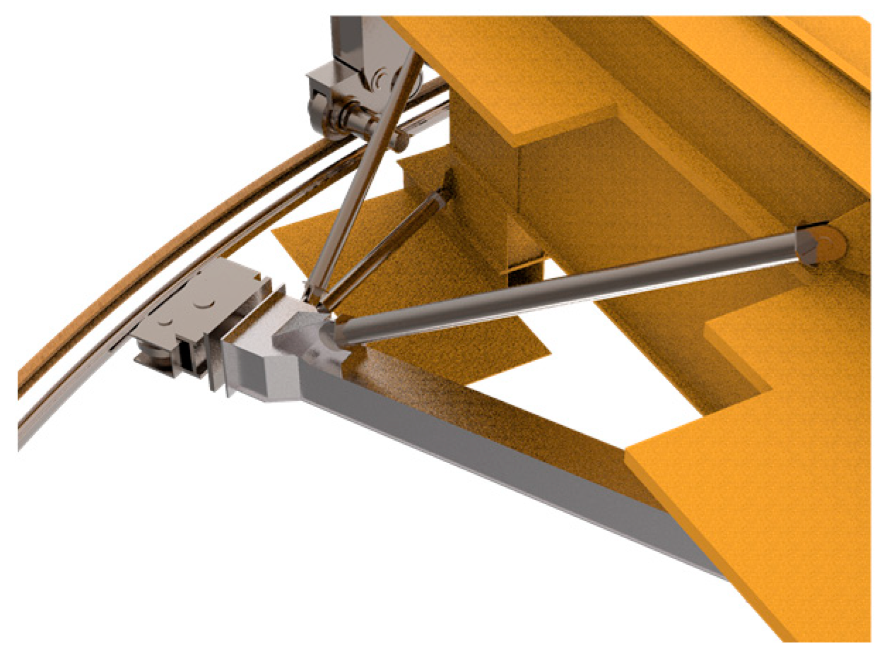
2.2.2. Dynamic Analysis of the Horizontal Guide Device

As shown in Figure 3, horizontal guide devices are installed at every corner of the crane bridge, which are mainly composed of a horizontal guide outrigger, an oblique rod, a horizontal rod, and horizontal guide wheels. Furthermore, the horizontal guide wheels are connected to the outrigger by disc springs.

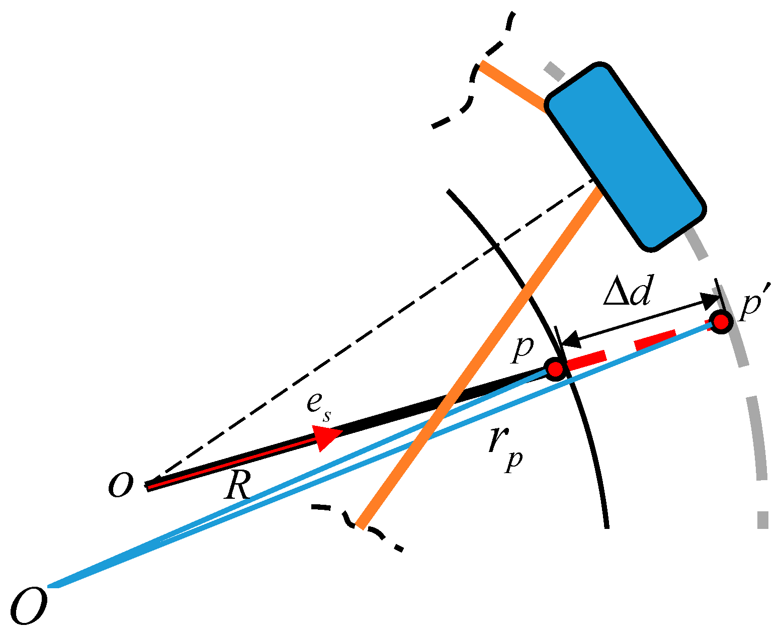
For ease of calculation, invasion between the horizontal guide wheel and the rail is allowed, so that the invasion distance can be used instead of the compression of the disc spring. Figure 4 shows the kinematic relationship of the horizontal guide device, where $p$ is the contact point of the horizontal guide wheel and the rail, $p^{\prime }$ is the invasion point, ${\mathit{e}}_{\mathit{s}}$ is the unit vector along the horizontal guide outrigger, $\Delta \mathrm{d}$ is the invasion distance, and $R$ is the radius of the rail.

Referring to [22], the kinematic relationship can be expressed as follows:

$$\Vert {\mathit{r}}_{\mathit{p}}-△\mathrm{d}{\mathit{e}}_{\mathit{s}}\Vert =R,$$

(13)

From Equation (13), the invasion distance can be obtained as follows:

$$\Delta \mathrm{d}=b-\sqrt{b^2-c},$$

(14)

where $b={\mathit{r}}_{\mathit{p}}\cdot {\mathit{e}}_{\mathit{s}}$ and $c={\mathit{r}}_{\mathit{p}}\cdot {\mathit{r}}_{\mathit{p}}-R^2$.

Therefore, the contact forces of the horizontal guide wheels can be written as follows:

$${\mathit{F}}_{{\mathit{n}}_{\mathit{i}}}=-f_{n_i}{\mathit{e}}_{\mathit{s}}^{\mathit{i}},i=1,2,3,4,$$

(15)

where $f_{n_i}$ is the magnitude of the contact force, which can be confirmed based on the relationship between invasion distance $\Delta \mathrm{d}$ and stiffness coefficient of the disc spring and where ${\mathit{e}}_{\mathit{s}}^{\mathit{i}}$ is the unit vector of each horizontal guide outrigger.

From the above analysis, the contact forces can be written in a vector form:

$${\mathit{F}}_{\mathit{n}}={\left[n_1,n_2,0,0,0,0,0\right]}^T,$$

(16)

where

$$n_1={\mathit{F}}_{{\mathit{n}}_1}\cos \left(\theta +{\delta }_2\right)-{\mathit{F}}_{{\mathit{n}}_2}\cos \left(\theta -{\delta }_2\right)-{\mathit{F}}_{{\mathit{n}}_3}\cos \left(\theta +{\delta }_2\right)+{\mathit{F}}_{{\mathit{n}}_4}\cos \left(\theta -{\delta }_2\right),$$

$$n_2={\mathit{F}}_{{\mathit{n}}_1}\sin \left(\theta +{\delta }_2\right)-{\mathit{F}}_{{\mathit{n}}_2}\sin \left(\theta -{\delta }_2\right)-{\mathit{F}}_{{\mathit{n}}_3}\sin \left(\theta +{\delta }_2\right)+{\mathit{F}}_{{\mathit{n}}_4}\sin \left(\theta -{\delta }_2\right),$$

Moreover, the frictional force between the horizontal guide wheel and the rail can be expressed as follows:

$${\mathit{F}}_{{\mathit{s}}_{\mathit{i}}}=-\mu f_{n_i}\frac{{\mathit{v}}_{{\mathit{p}}_{\mathit{i}}}}{\Vert {\mathit{v}}_{{\mathit{p}}_{\mathit{i}}}\Vert },i=1,2,3,4,$$

(17)

where $\mu$ is the rolling friction coefficient between the horizontal guide wheel and the rail and ${\mathit{v}}_{p_i}$ is the tangential velocity of the horizontal guide wheel.

Similarly, the frictional forces can be written in a vector form as follows:

$${\mathit{F}}_{\mathit{s}}={\left[s_1,s_2,s_3,0,0,0,0\right]}^T,$$

(18)

where

$$s_1=-{\mathit{F}}_{{\mathit{s}}_1}\sin \left(\theta +{\delta }_2\right)+{\mathit{F}}_{{\mathit{s}}_2}\sin \left(\theta -{\delta }_2\right)+{\mathit{F}}_{{\mathit{s}}_3}\sin \left(\theta +{\delta }_2\right)-{\mathit{F}}_{{\mathit{s}}_4}\sin \left(\theta -{\delta }_2\right),$$

$$s_2={\mathit{F}}_{{\mathit{s}}_1}\cos \left(\theta +{\delta }_2\right)-{\mathit{F}}_{{\mathit{s}}_2}\cos \left(\theta -{\delta }_2\right)-{\mathit{F}}_{{\mathit{s}}_3}\cos \left(\theta +{\delta }_2\right)+{\mathit{F}}_{{\mathit{s}}_4}\cos \left(\theta -{\delta }_2\right),$$

$$s_3={\displaystyle \sum _{i=1}^4{\mathit{F}}_{{\mathit{s}}_{\mathit{i}}}}\cdot l,$$

2.3. Simulation and Verification of the Crane System

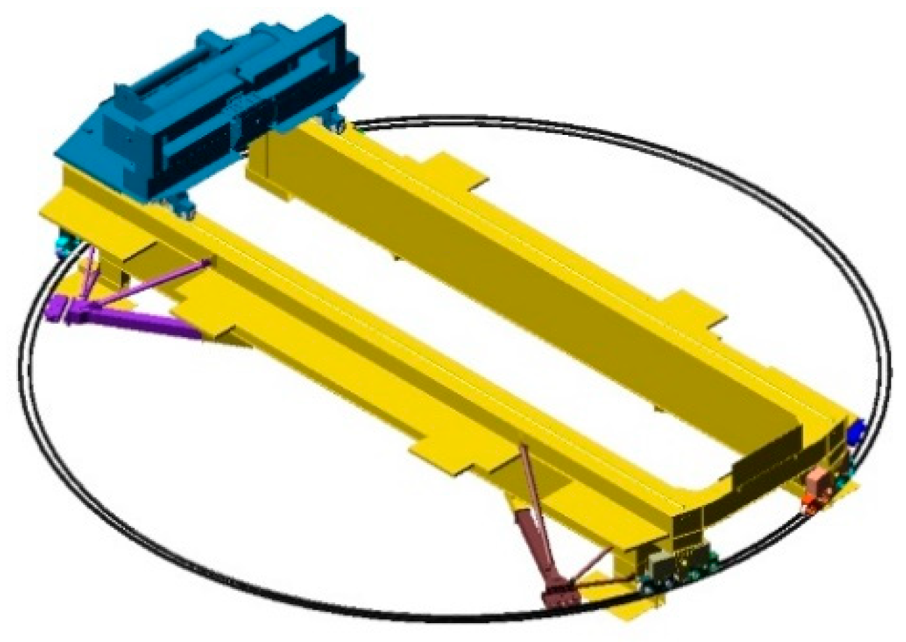
To verify the crane system depicted by the aforementioned equations, the simulation results of the crane system in MATLAB are compared with the results obtained from the crane system modeled in ADAMS software.

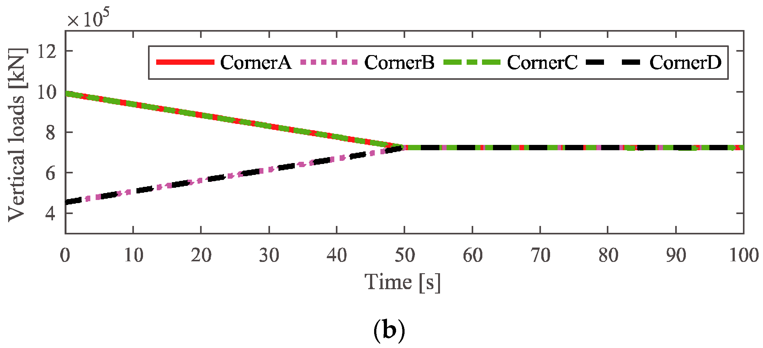
To this end, by using the modeled polar crane in ADAMS software, as shown in Figure 5, the crane system is simulated in a typical working condition, in which the movement states of the crane can be expressed as follows:

$$\begin{array}{ll}d=\{\begin{array}{l}20.5-0.41t\\ 0\end{array}& \begin{array}{c}0\le t<50\\ 50\le t\le 100\end{array}\\ {\dot{\phi }}_i=0.25\mathrm{rad}/\mathrm{s}& i=1,2,3,4\end{array},$$

(19)

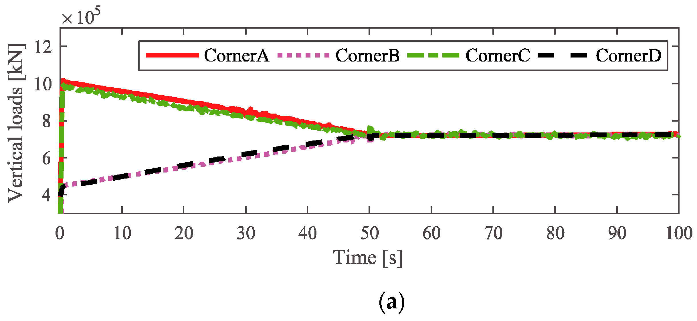
where an equal angular velocity $0.25\mathrm{rad}/\mathrm{s}$ is applied to the driving wheels of the bridge truck and the trolley starts to move from the end of crane bridge ($d=20.5\mathrm{m}$) at $0.41\mathrm{m}/\mathrm{s}$ and then stops at the center of crane bridge ($d=0\mathrm{m}$). The vertical loads of the driving wheels during crane operation are shown in Figure 6.

As it can be seen in the illustrations, although the vertical loads of the driving wheels obtained by using the proposed model and ADAMS are almost the same, there are still some slight differences; the main reasons for this are the differences in the wheel–rail contact conditions and structure simplification of the proposed theoretical model.

3. Control Scheme Design and Stability Analysis

Considering the location deviation between the geometric center of the crane and the center of rail, a NTSM-ADRC-QP-based control scheme is designed for the polar crane in this section.

3.1. ADRC-Based Decoupling Method

According to the dynamic equations of polar crane, as shown in Equation (7), the dynamic equations without Lagrange multipliers can be derived as follows:

$$\{\begin{array}{l}\left(M+m\right){\ddot{x}}_c+md\ddot{\theta }\sin \theta +md{\dot{\theta }}^2\cos \theta =F_x+\frac{J_{\omega }}{r}\left[{\ddot{\phi }}_1\mathbf{sin}(\theta +{\delta }_1)-{\ddot{\phi }}_2\mathbf{sin}(\theta -{\delta }_1)-{\ddot{\phi }}_3\mathbf{sin}(\theta +{\delta }_1)+{\ddot{\phi }}_4\mathbf{sin}(\theta -{\delta }_1)\right]+{\mathit{B}}_{\mathit{x}}\mathit{u}\hfill \\ \left(M+m\right){\ddot{y}}_c-md\ddot{\theta }\cos \theta +md{\dot{\theta }}^2\sin \theta =F_y+\frac{J_{\omega }}{r}\left[-{\ddot{\phi }}_1\mathbf{cos}(\theta +{\delta }_1)+{\ddot{\phi }}_2\mathbf{cos}(\theta -{\delta }_1)+{\ddot{\phi }}_3\mathbf{cos}(\theta +{\delta }_1)-{\ddot{\phi }}_4\mathbf{cos}(\theta -{\delta }_1)\right]+{\mathit{B}}_{\mathit{y}}\mathit{u}\hfill \\ m{\ddot{x}}_{c}d\sin \theta -m{\ddot{y}}_{c}d\cos \theta +\left(\frac{m^2{d}^2}{M+m}+J_d\right)\ddot{\theta }=M_{\theta }-\frac{R{J}_{\omega }}{r}{\displaystyle \sum _{i=1}^4{\ddot{\phi }}_i+{\mathit{B}}_{\mathbf{\theta }}\mathit{u}}\hfill \end{array},$$

(20)

where

$${\mathit{B}}_{\mathit{x}}=\frac{1}{r}\left[\begin{array}{cccc}-\sin \left(\theta +{\delta }_1\right)& \sin \left(\theta -{\delta }_1\right)& \sin \left(\theta +{\delta }_1\right)& -\sin \left(\theta -{\delta }_1\right)\end{array}\right],$$

$${\mathit{B}}_{\mathit{y}}=\frac{1}{r}\left[\begin{array}{cccc}\cos \left(\theta +{\delta }_1\right)& -\cos \left(\theta -{\delta }_1\right)& -\cos \left(\theta +{\delta }_1\right)& \cos \left(\theta -{\delta }_1\right)\end{array}\right],$$

$${\mathit{B}}_{\mathbf{\theta }}=\left[\begin{array}{cccc}\frac{R}{r}& \frac{R}{r}& \frac{R}{r}& \frac{R}{r}\end{array}\right],$$

$$\mathit{u}={\left[\begin{array}{cccc}{u}_1& u_2& u_3& u_4\end{array}\right]}^T,$$

Through a simple transformation, Equation (20) can be modified as follows:

$$\{\begin{array}{l}{\ddot{x}}_c=f_1\left(\overline{q},\dot{\overline{q}},{\ddot{\phi }}_1,{\ddot{\phi }}_2,{\ddot{\phi }}_3,{\ddot{\phi }}_4,w_1,t\right)+U_1\hfill \\ {\ddot{y}}_c=f_2\left(\overline{q},\dot{\overline{q}},{\ddot{\phi }}_1,{\ddot{\phi }}_2,{\ddot{\phi }}_3,{\ddot{\phi }}_4,w_2,t\right)+U_2\hfill \\ \ddot{\theta }=f_3\left(\overline{q},\dot{\overline{q}},{\ddot{\phi }}_1,{\ddot{\phi }}_2,{\ddot{\phi }}_3,{\ddot{\phi }}_4,w_3,t\right)+U_3\hfill \end{array},$$

(21)

where $\overline{q}=\left(x_c,y_c,\theta \right)$; $w_1$, $w_2$, and $w_3$ are uncertainty disturbances; $f_1$, $f_2$, and $f_3$ can be regard as total disturbance items including uncertainty disturbance and nonlinear coupling disturbance; and $U_1$, $U_2$, and $U_3$ are virtual control items. Therefore, the crane dynamic system with single-input single-output relationships is formed.

In this section, the decoupling control scheme of crane system is hierarchically designed according to the ADRC method. It is used for disturbance estimation and compensation in real time. The quadratic programming algorithm is used for active torques distribution, and the decoupling control scheme is shown in Figure 7.

ADRC is composed of three parts: tracking differentiator (TD), ESO, and nonlinear state error feedback (NLSEF). For safety reasons in crane operation, the saturation of the virtual control items $U_i$ is taken into consideration in the design of ADRC; taking the generalized coordinate $x_c$ as an example, the control structure is shown in Figure 8.

3.1.1. ESO Design

Based on Equation (21), the state-space model of the generalized coordinate $x_c$ can be expressed as follows:

$$\{\begin{array}{l}{\dot{x}}_1=x_2\hfill \\ {\dot{x}}_2=f_1\left(\overline{q},\dot{\overline{q}},{\ddot{\phi }}_1,{\ddot{\phi }}_2,{\ddot{\phi }}_3,{\ddot{\phi }}_4,w_1,t\right)+U_1\hfill \\ x_c=x_1\hfill \\ U_1=sat\left({\widehat{U}}_0\right)\hfill \end{array},$$

(22)

where the function $sat\left({\widehat{U}}_0\right)$ is used to depict the saturation of $U_1$ and the function $sat\left({\widehat{U}}_0\right)$ is defined as follows:

$$U_1=sat\left({\widehat{U}}_0\right)=\{\begin{array}{cc}{\widehat{U}}_0\hfill & \hfill \left|{\widehat{U}}_0\right|<U_{\max }\\ \mathrm{sign}\left({\widehat{U}}_0\right)U_{\max }\hfill & \hfill \left|{\widehat{U}}_0\right|\ge U_{\max }\end{array},$$

(23)

where $U_{\max }>0$ is the maximum value of the $U_1$.

Regarding $f_1$ as a new state variable, Equation (22) can be expanded into the following control system:

$$\{\begin{array}{l}{\dot{x}}_1=x_2\hfill \\ {\dot{x}}_2=x_3+U_1\hfill \\ {\dot{x}}_3=h\hfill \\ x_c=x_1\hfill \\ U_1=sat\left({\widehat{U}}_0\right)\hfill \end{array},$$

(24)

Here, we define $h={\dot{f}}_1$, $h$ as unknown but bounded. Referring to [23,24,25], the ESO can be constructed as follows:

$$\{\begin{array}{l}{\epsilon }_1=z_1-x_c\hfill \\ {\dot{z}}_1=z_2-{\alpha }_{01}{\epsilon }_1\hfill \\ {\dot{z}}_2=z_3-{\alpha }_{02}fal\left({\epsilon }_1,a_1,{\sigma }_1\right)+{\widehat{U}}_1\hfill \\ {\dot{z}}_3=-{\alpha }_{03}fal\left({\epsilon }_1,a_2,{\sigma }_2\right)\hfill \end{array},$$

(25)

where $z_1$ and $z_2$ are the estimates of $x_1$ and $x_2$, respectively; $z_3$ is the estimate of the total disturbance $f_1$; ${\epsilon }_1$ is the estimation error of $z_1$; and ${\alpha }_{01}$, ${\alpha }_{02}$, and ${\alpha }_{03}$ are the gain coefficients. In addition, $a_1$, $a_2$, ${\sigma }_1$, and ${\sigma }_2$ are the tunable parameters of the function $fal\left(\epsilon ,a,\sigma \right)$, and the function $fal\left(\epsilon ,a,\sigma \right)$ is defined as follows:

$$fal\left(\epsilon ,a,\sigma \right)=\{\begin{array}{cc}\epsilon /{\sigma }^{1-a},\hfill & \hfill \left|\epsilon \right|\le \sigma \\ {\left|\epsilon \right|}^a\mathrm{sign}\left(\epsilon \right),\hfill & \hfill \left|\epsilon \right|>\sigma \end{array},$$

(26)

Due to the saturation, the actual input of the ESO can be expressed as follows:

$${\widehat{U}}_1=-k_{U_1}\Delta {\widehat{U}}_0+{\widehat{U}}_0,$$

(27)

where $\Delta {\widehat{U}}_0={\widehat{U}}_0-U_1$ is the saturation error and $k_{U_1}$ is the compensation coefficient.

By properly selecting the value of the observer parameters, the outputs of the ESO can estimate well the state variables of the crane system.

3.1.2. Design of Nonsingular Terminal Sliding Mode Control

To improve the robustness and convergence speed of the control scheme, the NTSM is introduced into the ADRC method instead of the traditional nonlinear state error feedback. According to Equation (22), the state-space model of the tracking error of the generalized coordinate $x_c$ can be expressed as follows:

$$\{\begin{array}{l}{\dot{e}}_1=e_2\hfill \\ {\dot{e}}_2=f_1+U_1=f_1+{\widehat{U}}_0-\Delta {\widehat{U}}_0\hfill \\ e_1=x_1-x_0\hfill \end{array},$$

(28)

Referring to [26,27,28], the nonsingular terminal sliding surface can be constructed as follows:

$$s=e_1+{\lambda }_x{\left|e_2\right|}^{{\gamma }_x}\mathrm{sign}\left(e_2\right),$$

(29)

where ${\lambda }_x$ and ${\gamma }_x$ are tunable parameters and satisfy ${\lambda }_x>0$ and $1<{\gamma }_x<2$.

Accordingly, the control law can be expressed as follows:

$${\widehat{U}}_0=u_{eq}+u_n,$$

(30)

where $u_{eq}$ is the equivalent control item and $u_n$ is the nonlinear control item.

The differential of $s$ can be obtained as follows:

$$\dot{s}=e_2+{\lambda }_x{\gamma }_x{\left|e_2\right|}^{{\gamma }_x-1}\left(f_1+{\widehat{U}}_0-\Delta {\widehat{U}}_0\right),$$

(31)

Let $\dot{s}=0$. The equivalent control item $u_{eq}$ can be obtained as follows:

$$u_{eq}=-\left[\frac{1}{{\lambda }_x{\gamma }_x}{\left|e_2\right|}^{2-{\gamma }_x}\mathrm{sign}\left(e_2\right)+f_1-\Delta {\hat{U}}_0\right],$$

(32)

Moreover, an exponential reaching law, $\dot{s}=-c_1\tanh \left(s\right)-c_{2}s$, is introduced to restrain the chattering [29], and according to the described exponential reaching law, the nonlinear control term can be constructed as follows:

$$u_n=-c_1\tanh \left(s\right)-c_{2}s,$$

(33)

where $c_1$ and $c_2$ are control parameters and satisfy $c_1>0$ and $c_2>0$.

Substituting Equations (32) and (33) into Equation (30), the specific form of the control law can be obtained:

$${\widehat{U}}_0=-\left[\frac{1}{{\lambda }_x{\gamma }_x}{\left|e_2\right|}^{2-{\gamma }_x}\mathrm{sign}\left(e_2\right)+f_1-\Delta {\widehat{U}}_0+c_1\tanh \left(s\right)+c_{2}s\right],$$

(34)

where the disturbance item $f_1$ and saturation error $\Delta {\widehat{U}}_0$ can be estimated and compensated by the ESO. Note the reference value $x_0={\dot{x}}_0=0$; thus, the control law of the NTSM can be further constructed by using the estimates $z_1$, $z_2$, and $z_3$ of the ESO:

$$\{\begin{array}{l}{U}_0=-\left[\frac{1}{{\lambda }_x{\gamma }_x}{\left|z_2\right|}^{2-{\gamma }_x}\mathrm{sign}\left(z_2\right)+c_1\tanh \left(s\right)+c_{2}s\right]\hfill \\ {\widehat{U}}_0=-z_3+U_0\hfill \end{array},$$

(35)

3.2. Stability Analysis

The following Lyapunov function is considered:

$$V=\frac{1}{2}{s}^2,$$

(36)

The differential of the above equation can be obtained as follows:

$$\begin{array}{cc}\hfill \dot{V}& =s\dot{s}=s\left\{e_2+{\lambda }_x{\gamma }_x{\left|e_2\right|}^{{\gamma }_x-1}\left(f_1+{\widehat{U}}_0-\Delta {\widehat{U}}_0\right)\right\}\hfill \\ & =s\left\{e_2+{\lambda }_x{\gamma }_x{\left|e_2\right|}^{{\gamma }_x-1}\left[f_1-\Delta {\widehat{U}}_0-\left(\frac{1}{{\lambda }_x{\gamma }_x}{\left|e_2\right|}^{2-{\gamma }_2}\mathrm{sign}\left(e_2\right)+f_1-\Delta {\widehat{U}}_0+c_1\tanh \left(s\right)+c_{2}s\right)\right]\right\}\hfill \\ & =-{\lambda }_x{\gamma }_x{\left|e_2\right|}^{{\gamma }_x-1}\left[c_{1}s\tanh \left(s\right)+c_2{s}^2\right]\hfill \end{array},$$

(37)

When $s\ne 0$, since ${\lambda }_x>0$ and $1<r_2<2$, then $\frac{r_2}{{\lambda }_2}{\left|x_2\right|}^{r_2-1}\ge 0$ and $\dot{V}\le 0$. Therefore, the NTSM control system is stable in the Lyapunov sense.

3.3. Design of Quadratic Programming Algorithm

In this section, the quadratic programming algorithm is used to solve the redundant actuation of the polar crane. Due to the contact force of the horizontal guide device being related to the trajectory deviation of the driving wheel, we also take stability and smoothness of the control torques into consideration; thus, we construct the quadratic program as follows:

$$\mathbf{min}J=\frac{1}{2}\Delta {\mathit{u}}^T\mathit{H}\Delta \mathit{u}+\mathit{Q}\mathit{u},$$

(38)

where $\Delta \mathit{u}\mathbf{=}\mathit{u}\left(t\right)-\mathit{u}\left(t-T\right)$ denotes the differences between the current control torques and the previous control torques, $\mathit{H}$ and $\mathit{Q}$ are the weight matrices, and $\mathit{H}$ is positively defined.

According to Equation (20), the constraint relationships between control torque $u_i$ and virtual control item $U_i$ can be expressed as follows:

$$\{\begin{array}{l}{\mathit{B}}_{\mathit{x}}\mathit{u}=U_1\hfill \\ {\mathit{B}}_{\mathit{y}}\mathit{u}=U_2\hfill \\ {\mathit{B}}_{\mathbf{\theta }}\mathit{u}=U_3\hfill \end{array},$$

(39)

Therefore, the optimization problem of redundant actuation of the polar crane can be rewritten in a quadratic form:

$$\begin{array}{l}\mathbf{min}J=\frac{1}{2}\Delta {\mathit{u}}^T\mathit{H}\Delta \mathit{u}+{\mathit{Q}}^T\mathit{u}\\ \mathrm{s}.\mathrm{t}.\mathit{B}\mathit{u}=\mathit{U}\\ u_{\min }\le u_i\le u_{\max }\end{array},$$

(40)

where $\mathit{H}$ is set to a $4\times 4$ unit matrix and the other matrices are constructed as follows:

$$\begin{gathered} \mathit{Q}={\left[\begin{array}{cccc}\frac{f_{n_1}}{{\displaystyle \sum _{i=1}^4{f}_{n_i}}}& \frac{f_{n_2}}{{\displaystyle \sum _{i=1}^4{f}_{n_i}}}& \frac{f_{n_3}}{{\displaystyle \sum _{i=1}^4{f}_{n_i}}}& \frac{f_{n_4}}{{\displaystyle \sum _{i=1}^4{f}_{n_i}}}\end{array}\right]}^T, \\ \mathit{B}={\left[\begin{array}{ccc}{\mathit{B}}_{\mathit{x}}& {\mathit{B}}_{\mathit{y}}& {\mathit{B}}_{\mathbf{\theta }}\end{array}\right]}^T, \\ \mathit{U}={\left[\begin{array}{ccc}{U}_1& U_2& U_3\end{array}\right]}^T, \end{gathered}$$

Finally, the control torques of the driving wheels can be obtained by solving this optimization problem.

4. Simulation Results and Discussion

In order to verify the effectiveness of the NTSM-ADRC-QP control scheme proposed in this paper, MATLAB/Simulink software is used for the simulations. The detailed dynamics parameters of the simulation model are shown in

Table 2. Parameters of the simulation model.

Symbol	Value	Symbol	Value
$L_1\left(\mathrm{m}\right)$	$39.8$	$m\left(\mathrm{kg}\right)$	$3.31\times {10}^5$
$L_2\left(\mathrm{m}\right)$	$10$	$r\left(\mathrm{m}\right)$	$0.395$
$l\left(\mathrm{m}\right)$	$20.5$	${\delta }_1(°)$	$14$
$R\left(\mathrm{m}\right)$	$20.5$	${\delta }_2(°)$	$30$
$M\left(\mathrm{kg}\right)$	$6.59\times {10}^5$	$d\left(\mathrm{m}\right)$	$-17\sim 17$

. Considering the structural characteristics of the system, there are two typical working conditions of the polar crane implemented to verify the performance of the proposed control scheme and compared with the ADRC-QP method simultaneously.

The parameters of the ESO in the control scheme are as follows:

$${\alpha }_{01}=50,{\alpha }_{02}=100,{\alpha }_{03}=30$$

where the parameters of the ESO in the ADRC-QP control scheme are set to be consistent with those in the NTSM-ADRC-QP control scheme and the parameters of the sliding mode surfaces in each channel are as follows:

$$\begin{gathered} {\lambda }_x=0.003,{\gamma }_x=1.56 \\ {\lambda }_y=0.002,{\gamma }_y=1.68 \\ {\lambda }_{\theta }=0.1,{\gamma }_{\theta }=1.1 \end{gathered}$$

In addition, considering the safety of the crane rotation, the virtual control item $U_3$ is limited to $\pm 100\mathrm{kN}\cdot \mathrm{m}$.

4.1. Simulation Analysis of the Autonomous Operating of the Bridge Truck

In this section, in order to verify the locating performance of the proposed control scheme, we consider a typical working condition of the polar crane, in which the bridge truck rotates at a constant velocity.

The reference attitude of the polar crane can be expressed as follows:

$${\left[\begin{array}{ccc}{x}_0& y_0& {\theta }_0\end{array}\right]}^T={\left[\begin{array}{ccc}0& 0& 0.25t\end{array}\right]}^T$$

The initial attitude of the polar crane can be depicted as follows:

$${\left[\begin{array}{ccc}{x}_c& y_c& \theta \end{array}\right]}^T={\left[\begin{array}{ccc}0& 0& 0\end{array}\right]}^T$$

The distance between the trolley and the geometric center $P_c$ is as follows:

$$d=17$$

To verify the robustness of the system, here, we applied the following external disturbances of the driving wheels:

$${\tau }_1={\tau }_4=\{\begin{array}{cc}0.1t\hfill & \hfill 0\le t<10\\ 2-0.1\left(t-10\right)\hfill & \hfill 10\le t<20\end{array}$$

and

$${\tau }_2={\tau }_3=\{\begin{array}{cc}0.2t\hfill & \hfill 0\le t<10\\ 4-0.2\left(t-10\right)\hfill & \hfill 10\le t<20\end{array}$$

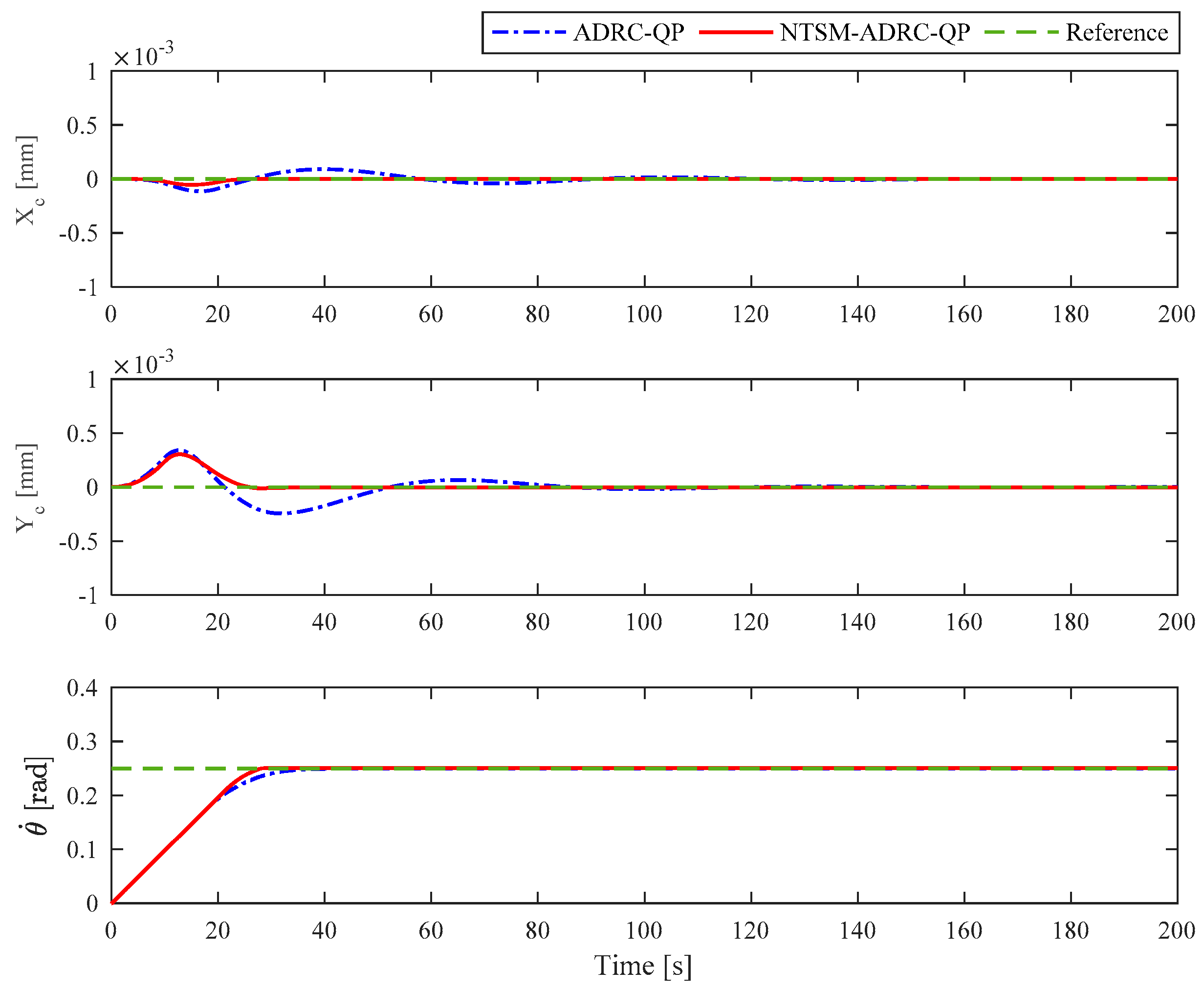
The locating performances of the polar crane in this working condition are illustrated in Figure 9, while the corresponding simulation results of the horizontal guide device and the driving wheel are shown in Figure 10, Figure 11 and Figure 12.

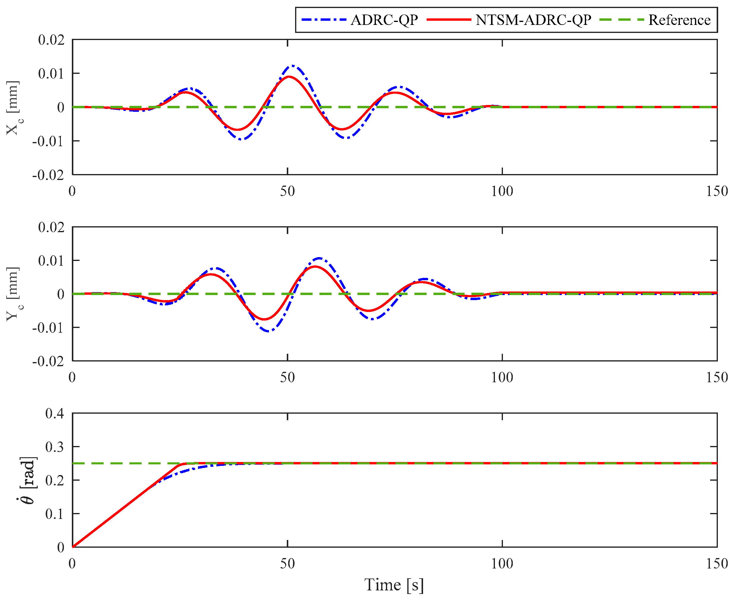
The locating performances of the two controllers are given in Figure 9. From Figure 9, it can be seen that the two controllers proposed in this paper are both able to ensure the locating accuracy very well, but in contrast, the convergence speed and robustness of the NTSM-ADRC-QP are obviously superior to the ADRC-QP. Figure 9 shows the rotation velocity of the polar crane, and the results show that the proposed control scheme can achieve the stable uniform rotation and the accurate locating simultaneously.

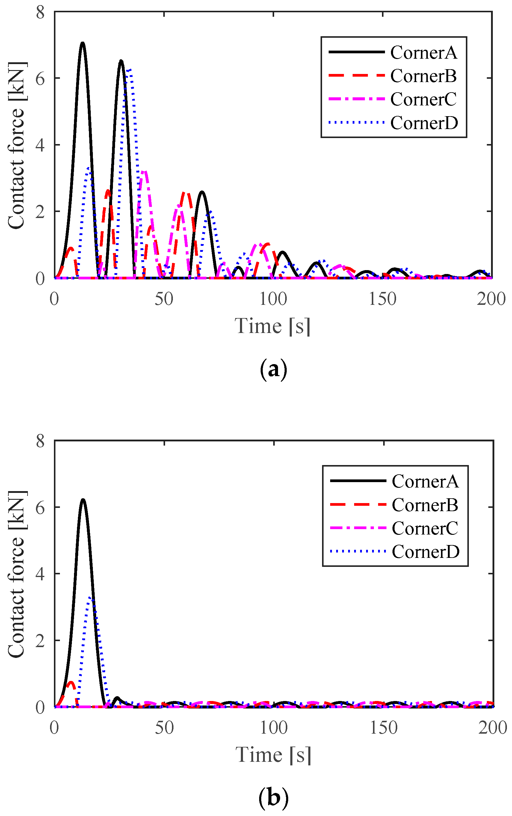
Figure 10 shows the contact forces of the horizontal guide devices; we can see that, compared with ADRC-QP, the contact forces of NTSM-ADRC-QP are obviously decreased. The main reason is that, as the location deviation decreases, the amount of compression between the horizontal guide wheel and the rail is accordingly decreased.

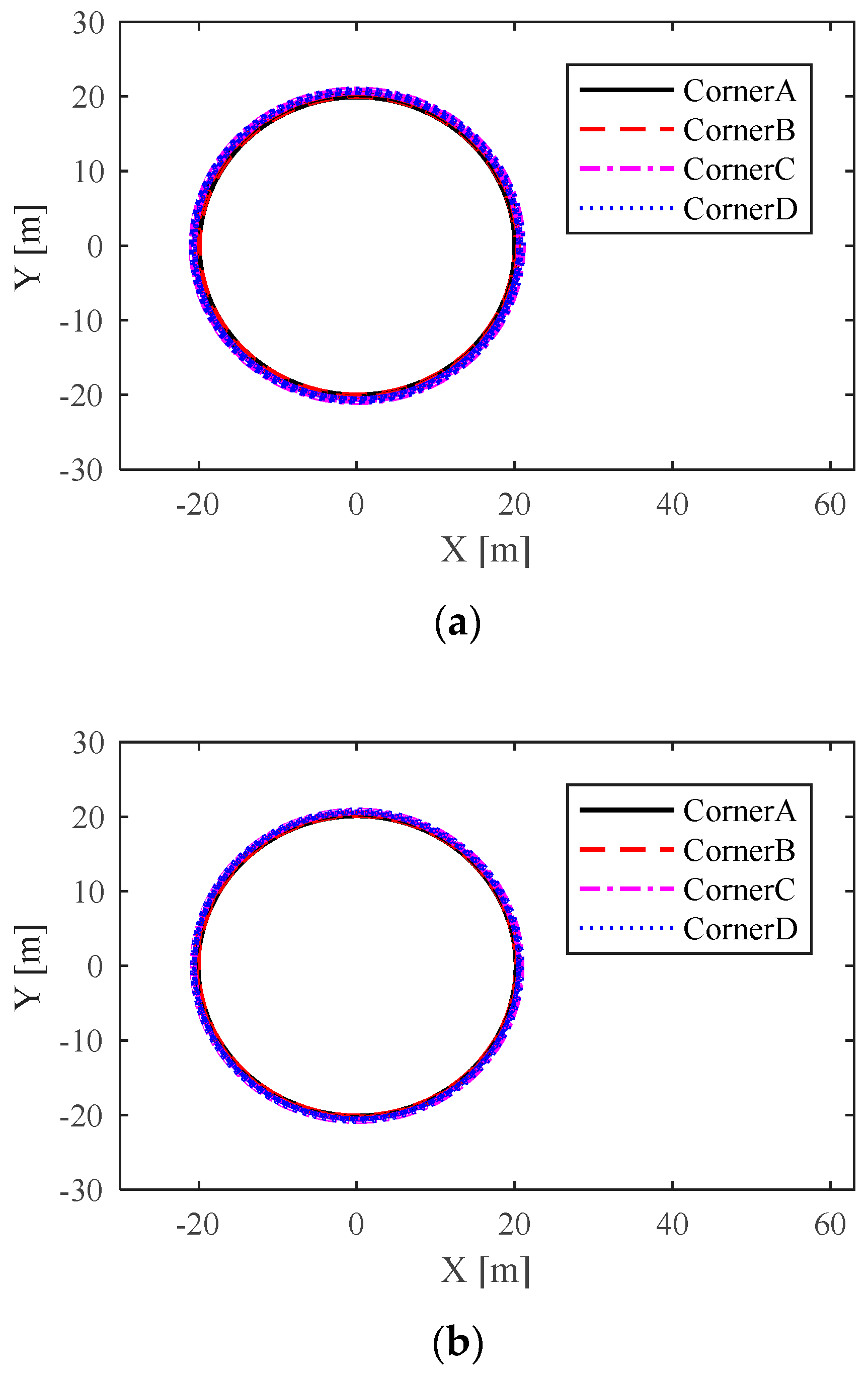
For direct observation, the moving trajectories of driving wheels at each corner are shown in Figure 11; note that the trajectory deviation of the driving wheels are amplified in the same proportion. It can be seen that the moving trajectories of the driving wheels via the NTSM-ADRC-QP control scheme are almost the same as the rail route, which reflects the remarkable control accuracy of the proposed NTSM-ADRC-QP control scheme directly.

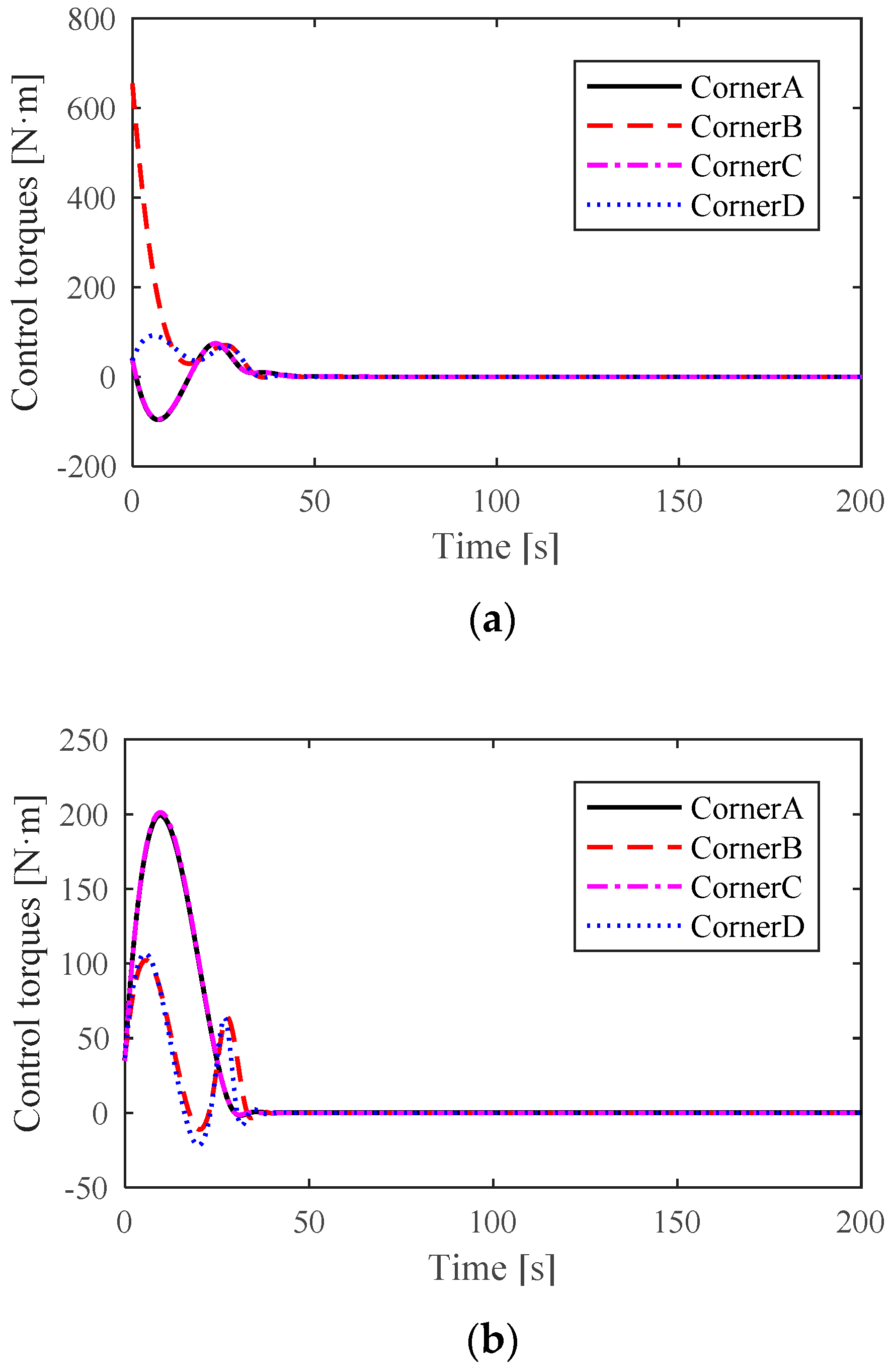
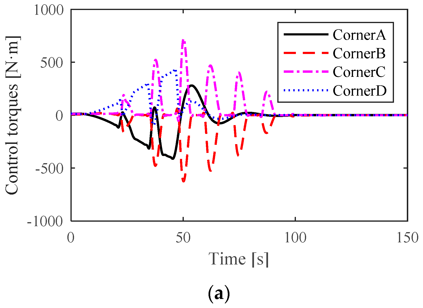
Figure 12 shows the distributed control torques of the driving wheels at each corner. It can be seen that the location deviation of the crane is close to zero before maintaining the uniform rotation, which reflects the robustness and effectiveness of the proposed control scheme. Furthermore, from the simulation results, note that the proposed quadratic program can effectively distribute the control torques and can thus improve the operational stability and control efficiency of the crane system.

4.2. Simulation Analysis of the Cooperative Operation

In this section, we focus on the effect of trolley movement on the crane locating performance, and the reference attitude and the initial attitude of the polar crane are set to be consistent with the above case; in this working condition, the distance between the trolley and the geometric center $P_c$ is as follows:

$$d=\{\begin{array}{cc}0.34t\hfill & \hfill 0\le t<50\\ 17-0.34\left(t-50\right)\hfill & \hfill 50\le t<100\end{array}$$

Note that the center of mass and the rotary inertia of the crane will change in response to the variation of the parameter $d$. The simulation results are shown in Figure 13, Figure 14, Figure 15 and Figure 16.

From Figure 13, it can be seen that the NTSM-ADRC-QP control scheme can still maintain fast convergence during crane operation, which reflects the better robustness of the designed control scheme. In addition, the simulation results further show that the movement of trolley has an important impact on crane location accuracy.

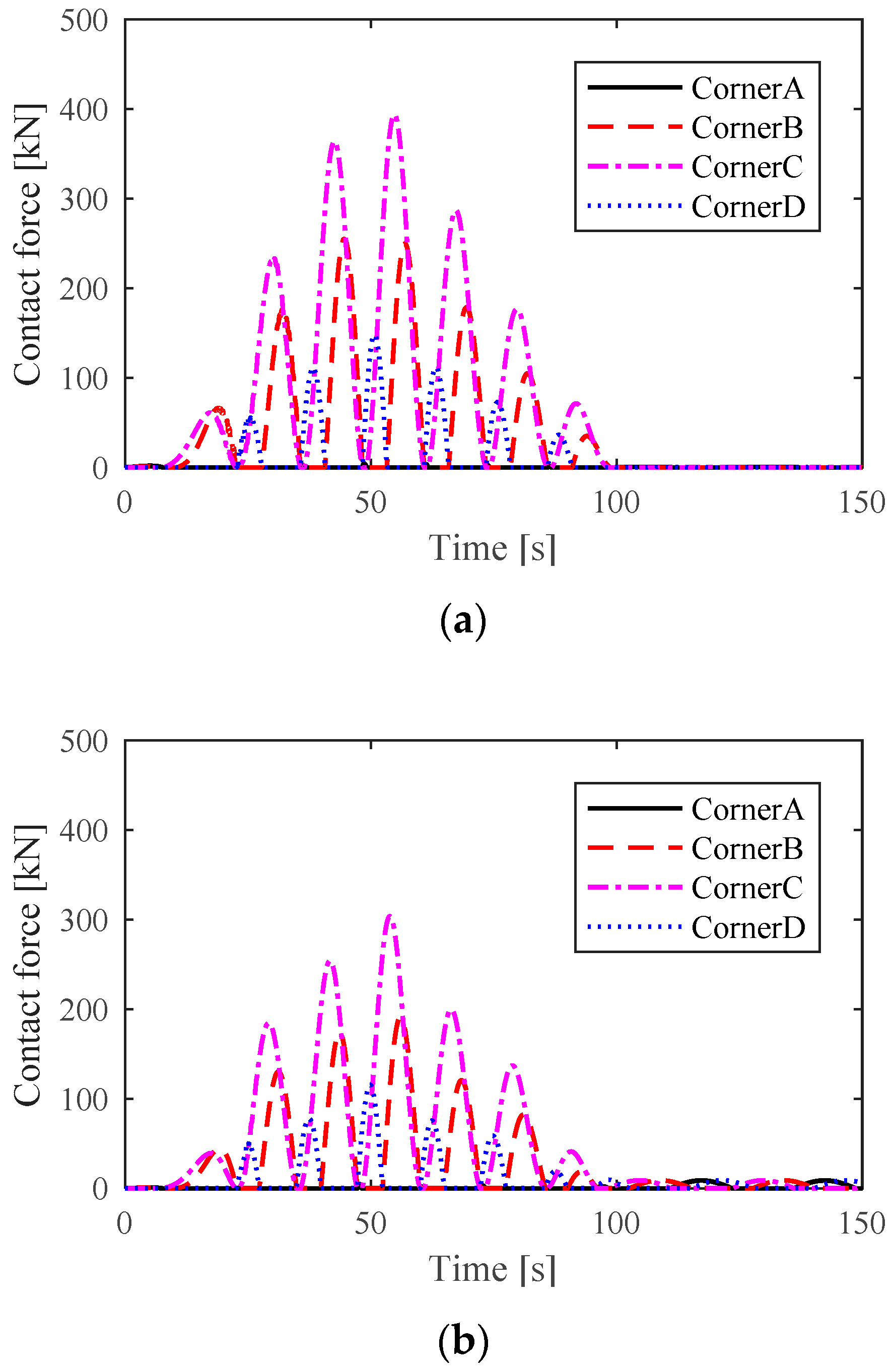
Figure 14 shows the contact forces of horizontal guide devices. We can see that the amplitude of the contact forces via the NTSM-ADRC-QP control scheme are decreased, which prove the robustness of the proposed control scheme on a side note.

Figure 15 shows the moving trajectories of the driving wheels at each corner. The simulation results are consistent with the results analyzed in Figure 13 and Figure 14. From the results, we can see that, under the center of mass and the rotary inertia changing, the moving trajectories of the driving wheels via NTSM-ADRC-QP are more precise.

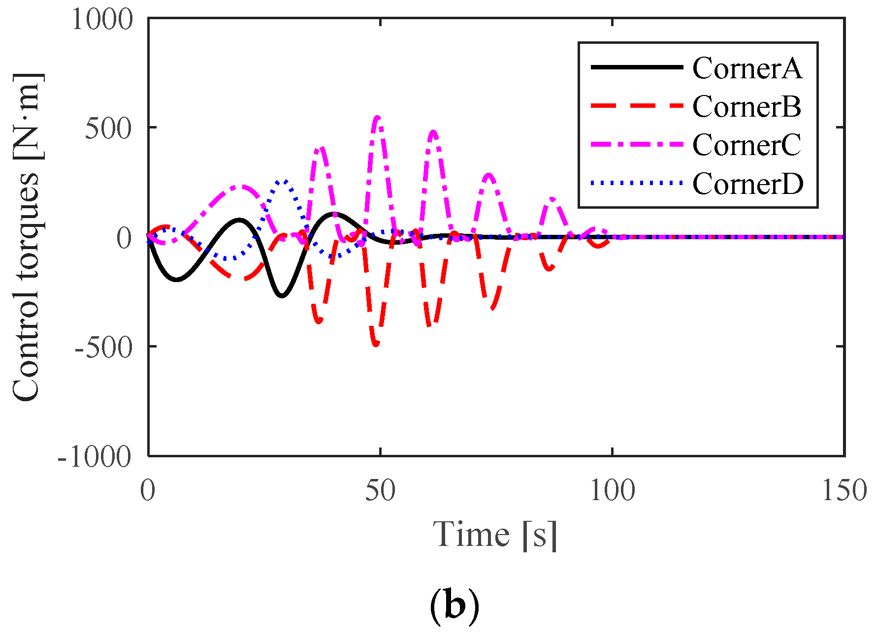
Figure 16 shows the distributed control torques of the driving wheels at each corner. In fact, based on the constraint relationships of the proposed quadratic programming algorithm, the variation in the location deviation will lead to variation in the control torques. Figure 16 manifests the adjustment process of the crane location deviation under the condition of uniform rotation.

5. Conclusions

In this paper, a novel locating control scheme is presented to address the problem of precise location for a polar crane. Based on the Lagrange–Rouse equation, a nonholonomic constraint dynamic model of the polar crane is established, and the ADRC-based decoupling control method is proposed to solve cross-coupling disturbance of the crane system. To improve the locating accuracy and robustness, the NTSM is incorporated with ADRC, and the stability of the control scheme is proved by the Lyapunov function approach. Additionally, a control torque distribution method based on the quadratic programming algorithm is designed to deal with the redundant actuation of the bridge truck. Considering the center of gravity shift during crane operation, two typical working conditions are simulated to verify the effectiveness of the proposed control scheme. The simulation results show that the proposed control scheme can achieve effective dynamic control of precise locations on the basis of uniform rotation.

In future work, we will further consider factors such as creep characteristics of wheel–rail contact and response delay of the driving wheel to improve the performance and safety of the control scheme. Furthermore, we will add the scale model test to verify the effectiveness of the proposed control scheme.

References

1. Zhaohui, Q.; Huitao, S.; Jing, W. Dynamic analysis of the rope-sheave system of polar crane for nuclear power plant. Proc. Inst. Mech. Eng. Part C J. Mech. Eng. Sci. 2018, 233, 269–286. [Google Scholar] [CrossRef]
2. Qi, Z.; Song, H.; Guo, S. Equilibrium path and load trajectory deflections for polar cranes in nuclear power plant. Adv. Mech. Eng. 2017, 9, 1–14. [Google Scholar] [CrossRef]
3. Cao, X.; Song, Y.; Qi, Z.; Yang, S. Research on straightness accuracy about hook assembly of the third-generation nuclear ring crane. J. Dalian Univ. Technol. 2013, 53, 51–57. [Google Scholar]
4. Qi, P.; Cao, X.; Lv, Y. The influence of the structural stiffness of the third-generation nuclear polar crane on precise positioning. Hoisting Conveying Mach. 2018, 17, 107–110. [Google Scholar] [CrossRef]
5. Deng, D.; Zhang, Y.; Zhen, R. Study on manufacturing process of ring-lifting corbel for nuclear power station. Hot Work. Technol. 2018, 47, 239–242, 246. [Google Scholar] [CrossRef]
6. Lv, Y.; Cao, X.; Gao, S. Study on rigid-flexible coupling dynamics simulation for the third-generation nuclear polar crane. Hoisting Conveying Mach. 2018, 17, 123–127. [Google Scholar] [CrossRef]
7. Ouyang, H.; Hu, J.; Zhang, G.; Mei, L.; Deng, X. Sliding-Mode-Based Trajectory Tracking and Load Sway Suppression Control for Double-Pendulum Overhead Cranes. IEEE Access 2018, 7, 4371–4379. [Google Scholar] [CrossRef]
8. Smoczek, J.; Szpytko, J. Particle Swarm Optimization-Based Multivariable Generalized Predictive Control for an Overhead Crane. IEEE/ASME Trans. Mechatron. 2017, 22, 258–268. [Google Scholar] [CrossRef]
9. Shao, X.; Zhang, J.; Zhang, X.-L. Takagi-Sugeno Fuzzy Modeling and PSO-Based Robust LQR Anti-Swing Control for Overhead Crane. Math. Probl. Eng. 2019, 2019, 1–14. [Google Scholar] [CrossRef]
10. Liu, H.; Chen, W.; Li, Y. Trajectory planning for crane’s trolley to suppress residual swing of payload. J. South China Univ. Technol. 2018, 46, 17–23. [Google Scholar] [CrossRef]
11. Wu, Z.; Xia, X. Optimal motion planning for overhead cranes. IET Control. Theory Appl. 2014, 8, 1833–1842. [Google Scholar] [CrossRef] [Green Version]
12. Peng, H.; Shi, B.; Wang, X.; Li, C. Interval estimation and optimization for motion trajectory of overhead crane under uncertainty. Nonlinear Dyn. 2019, 96, 1693–1715. [Google Scholar] [CrossRef]
13. Khatamianfar, A.; Savkin, A.V. Real-Time Robust and Optimized Control of a 3D Overhead Crane System. Sensors 2019, 19, 3429. [Google Scholar] [CrossRef] [PubMed] [Green Version]
14. Yang, T.; Sun, N.; Chen, H.; Fang, Y. Neural Network-Based Adaptive Antiswing Control of an Underactuated Ship-Mounted Crane With Roll Motions and Input Dead Zones. IEEE Trans. Neural Netw. Learn. Syst. 2020, 31, 901–914. [Google Scholar] [CrossRef] [PubMed]
15. Guo, B.; Chen, Y. Fuzzy robust fault-tolerant control for offshore ship-mounted crane system. Inf. Sci. 2020, 526, 119–132. [Google Scholar] [CrossRef]
16. Fang, Y.; Fang, Y. Switching Logic-Based Nonlinear Feedback Control of Offshore Ship-Mounted Tower Cranes: A Disturbance Observer-Based Approach. IEEE Trans. Autom. Sci. Eng. 2018, 16, 1125–1136. [Google Scholar] [CrossRef]
17. Wu, Z.; Guo, B. Active disturbance rejection control to MIMO nonlinear systems with stochastic uncertainties: Approximate decoupling and output-feedback stabilisation. Int. J. Control. 2018, 93, 1408–1427. [Google Scholar] [CrossRef]
18. Abdul-Adheem, W.R.; Ibraheem, I.K.; Azar, A.T.; Humaidi, A.J. Improved Active Disturbance Rejection-Based Decentralized Control for MIMO Nonlinear Systems: Comparison with the Decoupled Control Scheme. Appl. Sci. 2020, 10, 2515. [Google Scholar] [CrossRef] [Green Version]
19. Wang, Z.; Gong, Z.; Chen, Y.; Sun, M.; Xu, J. Practical control implementation of tri-tiltRotor flying wing unmanned aerial vehicles based upon active disturbance rejection control. Proc. Inst. Mech. Eng. Part G J. Aerosp. Eng. 2020, 234, 943–960. [Google Scholar] [CrossRef]
20. Jiang, L.; He, J. Control strategy and dynamic simulation of two-wheeled self-balancing vehicle. J. South China Univ. Technol. 2020, 44, 9–15. [Google Scholar]
21. Dong, Y.; Deng, Z.; Fang, H. Dynamics and Control Study of Rover with Six Wheels Independently Driven. J. Syst. Simul. 2009, 21, 1210–1213. [Google Scholar]
22. Zhang, X.; Qi, Z.; Wang, G.; Guo, S.; Qu, F. Numerical investigation of the seismic response of a polar crane based on linear complementarity formulation. Eng. Struct. 2020, 211, 110462. [Google Scholar] [CrossRef]
23. Gu, X.; Xu, W. Moving sliding mode controller for overhead cranes suffering from matched and unmatched disturbances. Trans. Inst. Meas. Control. 2020, 014233122092210. [Google Scholar] [CrossRef]
24. Coral-Enriquez, H.; Pulido-Guerrero, S.; Cortés-Romero, J. Robust Disturbance Rejection Based Control with Extended-state Resonant Observer for Sway Reduction in Uncertain Tower-cranes. Int. J. Autom. Comput. 2019, 16, 812–827. [Google Scholar] [CrossRef]
25. Cai, T.; Zhang, H.; Gu, L.; Gao, Z. On active disturbance rejection control of the payload position for gantry cranes. In Proceedings of the American Control Conference, Washington, DC, USA, 17–19 June 2013; pp. 425–430. [Google Scholar]
26. Wu, X.; Xu, K.; Lei, M.; He, X. Disturbance-Compensation-Based Continuous Sliding Mode Control for Overhead Cranes with Disturbances. IEEE Trans. Autom. Sci. Eng. 2020, 17, 2182–2189. [Google Scholar] [CrossRef]
27. Hoang, Q.; Park, J.; Lee, S.; Ryu, J. Aggregated Hierarchical Sliding Mode Control for Vibration Suppression of an Excavator on an Elastic Foundation. Int. J. Precis. Eng. Manuf. 2020, 21, 2263–2275. [Google Scholar] [CrossRef]
28. Ngo, Q.H.; Nguyen, N.P.; Nguyen, C.N.; Tran, T.H.; Bui, V.H. Payload pendulation and position control systems for an offshore container crane with adaptive-gain sliding mode control. Asian J. Control. 2020, 22, 2119–2128. [Google Scholar] [CrossRef]
29. Wu, Y.; Wang, L.; Zhang, J.; Li, F. Path Following Control of Autonomous Ground Vehicle Based on Nonsingular Terminal Sliding Mode and Active Disturbance Rejection Control. IEEE Trans. Veh. Technol. 2019, 68, 6379–6390. [Google Scholar] [CrossRef]
Figure 1. Overview of the polar crane.
Machines 09 00022 g001
Figure 2. Schematic of the polar crane system: (a) overview of the crane kinetic relationship and (b) local magnification of the crane geometric center.
Machines 09 00022 g002
Figure 3. Horizontal guide device.
Machines 09 00022 g003
Figure 4. Schematic of the horizontal guide device.
Machines 09 00022 g004
Figure 5. The polar crane modeled in ADAMS.
Machines 09 00022 g005
Figure 6. Response comparison of the vertical loads of the driving wheels: (a) simulation via ADAMS and (b) simulation via MATLAB.
Machines 09 00022 g006aMachines 09 00022 g006b
Figure 7. Schematic diagram of the decoupling control scheme, where x 0 , y 0 , and θ 0 are the reference values of the generalized coordinates x c , y c , and θ .
Machines 09 00022 g007
Figure 8. Error-compensation-based anti-saturation scheme for active disturbance rejection control (ADRC).
Machines 09 00022 g008
Figure 9. The comparison of locating performance of the two control schemes.
Machines 09 00022 g009
Figure 10. The comparison of the contact forces of the two control schemes: (a) contact forces via the ADRC-quadratic programming (QP) control scheme and (b) contact forces via the nonsingular terminal sliding mode (NTSM)-ADRC-QP control scheme.
Machines 09 00022 g010
Figure 11. The moving trajectory of the driving wheel: (a) moving trajectories of the driving wheels via the ADRC-QP control scheme and (b) moving trajectories of the driving wheels via the NTSM-ADRC-QP control scheme.
Machines 09 00022 g011
Figure 12. The control torques of the driving wheels: (a) control torques of the driving wheels via the ADRC-QP control scheme and (b) control torques of the driving wheels via the NTSM-ADRC-QP control scheme.
Machines 09 00022 g012
Figure 13. The comparison of the locating performances of the two control schemes.
Machines 09 00022 g013
Figure 14. The comparison of the contact forces of the two control schemes: (a) contact forces in the ADRC-QP control scheme and (b) contact forces in the NTSM-ADRC-QP control scheme.
Machines 09 00022 g014
Figure 15. The moving trajectory of the driving wheel: (a) moving trajectories of the driving wheels in the ADRC-QP control scheme and (b) moving trajectories of the driving wheels in the NTSM-ADRC-QP control scheme.
Machines 09 00022 g015
Figure 16. The control torques of the driving wheels: (a) control torques of the driving wheels via the ADRC-QP control scheme and (b) control torques of the driving wheels via the NTSM-ADRC-QP control scheme.
Machines 09 00022 g016aMachines 09 00022 g016b