1. Introduction
Artificial intelligence techniques are used throughout modern society for numerous applications. They have been used for gaming [
1], robotics [
2], credit worthiness decision-making [
3,
4], assisting in surgical procedures [
5,
6], cyberattack detection [
7] and numerous other applications. A key issue with some forms of artificial intelligence is a lack of human understanding of how the techniques work and the exact criteria upon which decisions are made. This issue is particularly pronounced when these systems make decisions which impact humans [
8]. Neural networks (see, e.g., [
9,
10]), in particular, have caused concern as their networks do not have a known meaning—instead, they are a temporary summation of the learning that has occurred to date [
11]. Moreover, the network could readily change if additional learning occurs. Concerns about understandability and unknown bias in decision-making have led to artificial intelligence techniques being called “algorithms of oppression” [
12] and the development of explainable techniques (see, e.g., [
13,
14]) that avoid some of these pitfalls.
Expert systems [
15,
16] are one of the earlier forms of artificial intelligence. They were introduced in the 1960s and 1970s with two key systems, Dendral and Mycin [
17]. They are inherently understandable as they utilize a rule-fact network. Initially, expert systems were designed to emulate what an expert in a field would do in making conclusions about specific data; however, expert systems have found use in numerous other areas, such as control systems [
18] and facial expression [
19] and power system [
20] analysis. Traditionally, expert systems have been implemented using an iterative algorithm that processes the rule-fact network. This approach is problematic in that the outcome of the network may be different depending on the order in which rules are selected for execution. Additionally, the iterative nature of the approach means that its decision-making time is unknown. This limitation impairs the utility of expert systems for robotics and other real-time applications.
One approach to removing these limitations is to implement expert systems in hardware where the rule execution logic can be performed truly in parallel (as opposed to simulated parallelism through timesharing or similar techniques). It has been proposed [
21,
22] that hardware-based gates be used in place of creating software-based rule-fact networks. The prior work [
21,
22], though, did not implement or validate hardware expert systems’ efficacy or performance.
This paper’s objective is to demonstrate the functionality and characterize the performance of hardware-based expert systems and to compare them to software-based ones. The contributions of this paper are the demonstration of the implementation of a hardware expert system (which was theorized, but not implemented, in prior work [
21,
22]), and the validation of their efficacy and the assessment of their performance. To this end, limitations on hardware expert systems network sizes are explored. Additionally, rule-fact expert system networks are developed in both software and hardware and their performance is compared.
This paper continues, in
Section 2, by reviewing prior work that provides a foundation for the work presented herein.
Section 3 details the system design that was used to model both the hardware and software-based expert system networks that were used for the experiments performed.
Section 4 presents the data collected via the testing of the types of networks and its analysis. Then, in
Section 5, applications and hardware expert system efficacy for them are discussed. Finally, the paper concludes in
Section 6 and discusses areas of potential future work.
2. Background
This section presents prior work on expert systems and their applications, as well as work related to the proposed concept of taking a hardware-based approach to implementing an expert system. First, a general overview of expert systems is presented. Following this, in
Section 2.2, expert systems’ potential use cases are described. In
Section 2.3, the use of artificial intelligence in robotics is discussed. Next, in
Section 2.4, prior work on explainable artificial techniques is reviewed. Finally,
Section 2.5 details how hardware-based expert systems have been previously theorized and assessed. It also discusses potential use cases and implementations of hardware-based expert systems.
2.1. Expert System
Expert systems are a form of artificial intelligence that was originally designed to emulate the behavior of a human expert within a specific field or application [
23]. Initially, these systems were developed using rule-fact networks [
15,
16] which were built based on knowledge collection from experts [
24]. Traditional expert systems utilize a rule-fact-based network to reach a conclusion based on given inputs [
24]. Simply, in these systems, facts can have either a true or a false value. The initial input facts serve as inputs to rules. If both input facts are identified as being true, then additional facts (the rule outputs) can also be asserted as true. The rule processing engine that operates an expert system scans the network for rules that have had their preconditions satisfied and updates any of the relevant output facts accordingly. Notably, the process used for rule selection is a key feature of expert system engines. The Rete algorithm, developed by Forgy [
25], gained prominence due to its capabilities for rule selection. Later versions of Rete, for which the underlying algorithms were not publicly disclosed, notably improved upon the initial algorithm’s performance [
26].
Beyond the traditional rule-fact expert systems, systems performing similar functions which use fuzzy logic [
27,
28,
29] and which are based on neural networks [
30,
31] have been proposed. Systems have also been developed which use the connection weights from a neural network to generate rules for expert systems’ rule-fact networks, rather than using a human knowledge engineer to develop the network [
27]. A system using neural network optimization principles directly on an expert system rule-fact network has also been proposed [
32].
2.2. Expert System Uses
Expert systems have been used in a wide variety of different fields and for different types of tasks. One area where expert systems have found a wide variety of uses is the medical field [
33]. Within the medical field, expert systems have been used and developed for diet planning [
34], diabetes therapy [
35], heart disease [
36], eye disease [
37], skin disease [
38], COVID-19 [
39] and hypertension [
40] diagnosis, lower back pain diagnosis and treatment [
33], neck pain diagnosis [
33] and many more have also been developed [
33] relating to medical diagnosis and treatment. Expert systems have also been used to diagnose diseases in fruits [
41], plants [
42] and animals [
43].
Beyond medicine and related fields, expert systems have also been used for numerous other applications including knowledge extraction [
44], construction [
45] and tourism [
46] planning, quality control [
47], fault detection [
48], power systems [
20], facial feature identification [
19], geographic information systems [
49] and agriculture [
50]. They have also found uses in education, such as for academic advising [
51], testing [
52] and projecting student performance [
53].
2.3. Artificial Intelligence in Robotics
Robotics is a key field where artificial intelligence concepts have been used. Machine learning, in particular, has been used to optimize robot performance through autonomous learning [
54]. Robots have been developed that are able to perform numerous tasks such as driving, flying, swimming and transporting items through various environments [
54]. One example of an application area where artificial intelligence is used within robotics is unmanned aerial vehicles (UAVs). UAVs themselves are used for numerous applications, including livestock [
55] and forest fire detection [
56], ensuring food security on farms [
57] and military applications [
54]. Artificial intelligence techniques have also been demonstrated for use in robot foraging [
58], robotic manufacturing [
59,
60], fault identification [
61] and diagnosis [
62].
Artificial intelligence has been implemented in robotics, using techniques such as deep learning and neural networks, to provide object recognition [
54,
56], interaction [
63] and avoidance [
64] capabilities. While artificial intelligence technologies have proved to be useful for object recognition, using neural networks and deep learning makes the systems difficult for humans to understand and troubleshoot, as the techniques are not inherently understandable [
8]. Artificial intelligence techniques have also been used for robotic command decision-making [
65] and managing connectivity and security, determining robot position and for other purposes [
66].
In addition to using neural networks and deep learning, other techniques, such as particle swarm optimization, have also been used for robotics. Particle swarm optimization, in particular, has been used for determining UAV trajectory and facilitating multi-robot communications [
66]. Machine learning has also been used within robotics for mobility prediction, virtual-reality-commanded operations and deployment optimization, among other things [
66]. Expert systems and the conceptually related Blackboard Architecture [
67] have been used for robotic command [
68]. Artificial intelligence is an integral part of robotics as many applications require capabilities beyond teleoperation which must be performed using artificial intelligence techniques. Despite the extensive use of artificial intelligence in robotics, numerous limitations still remain as many techniques are not deterministic with respect to time, making them problematic for controlling real-time autonomous robotic systems. Non-understandable techniques are also problematic for robotic (as well as other) uses, as discussed subsequently, as they cannot be guaranteed to perform appropriately in all circumstances. They are also not able to justify their decisions in cases of failure.
2.4. Explainable Artificial Intelligence
While expert systems have been around since the at least the 1970s [
17] (some would argue since the 1960s [
69], considering Dendral instead of Mycin to be the first expert system), the later growth in the prevalence of neural network use [
70] has led to issues that have driven the development of new types of artificial intelligence that strive to have expert systems’ inherent property of understandability. These techniques are called explainable artificial intelligence (XAI). They have been developed because neural networks have been shown to have issues related to poor transparency and bias and because they have the potential for learning non-causal relationships [
8]. Some are not able to even “explain their autonomous decisions to human users” [
13], despite their effectiveness at making them. XAI techniques seek to mitigate understandability problems by implementing techniques that facilitate human developers and users’ understanding of how autonomous systems are making their decisions [
13].
Arrieta et al. [
71] have categorized XAI into two categories: techniques that provide a “degree of transparency” and techniques which are “interpretable to an extent by themselves”. Expert systems fall into the interpretable by themselves category and are inherently human understandable due to their rule-fact network structure.
While XAI systems are a demonstrable advancement from opaque ones, Buhmann and Fieseler note that “simply the right to transparency will not create fairness” [
72]. Techniques such as expert systems that do not just explain how a decision was made but also constrain decisions to only valid outcomes are key to solving the problems identified by Buhmann and Fieseler.
2.5. Hardware Expert System
Hardware-based expert systems were proposed in [
21] and discussed in [
22]. Their performance was also projected in [
22]. While there are variations between hardware and software expert system implementations, a significant similarity exists between the rule-fact network structure of an expert system and circuits created using electronic AND-gates [
21]. A traditional expert system, whose inputs can have either true or false values, can—because of this similarity—be readily constructed electronically using hardware AND-gates [
22].
The use of a hardware-based expert system might prove to be effective for applications where a fixed rule-fact network would have numerous uses, where the reduced processing time required across multiple runs would compensate for the higher cost of physical network configuration. Thus, one use for electronic expert systems is for applications where the time benefits of hardware-based network performance outweigh the creation time and cost, in comparison to the much faster and cheaper production and time cost of a software-based expert system.
Notably, software-based systems require a computer to operate them. For applications where a computer is not already available or applications where the expert system’s needs drive the computational costs, hardware-based expert systems may also provide a financial benefit (in addition to a processing speed one).
A hardware-based network would operate in the same way as a traditional Boolean rule-fact network-based expert system that uses inputs that have either true or false values [
22]. The principal difference between the two is that a software-based expert system uses general purpose computational hardware to apply Boolean logic when processing the network to verify that rule prerequisites have been met and assert output facts. A hardware-based network instead uses electronic gates where signals are either a one-value (a HIGH digital signal) or a zero-value (a LOW digital signal). The two states that signals can be at parallels the rule-fact structure that an expert system relies on for network processing. This characteristic allows hardware-based implementations to provide all of the functionality of software-based systems while providing benefits over a software-based network, in applications where the network design is fixed. Due to the high setup and change-over costs, electronic implementations would not be practical for applications where the network changed frequently.
3. System Design
For data collection and testing, two types of networks were designed. The first type of networks were comprised of between one and five network components that each included 32 AND-gates. They were designed to measure the time it takes a signal to propagate through varying amounts of gates, based on how many network components were connected. The second type of networks were designed to model how a real-world network would work. They had different amounts of inputs, structures and network designs.
The underlying methodology behind the creation of each of the five networks for the second network type was to create different network configurations and complexities. Each type of network could have different potential bottlenecks and other considerations which could impact system performance. The networks’ designs first focused on some networks having more depth versus others having more breadth, both in terms of the number of required inputs and the configuration of facts and rules.
This design facilitated assessment as to whether a breadth-heavy network—one which had most of the inputs to the network required before later layers—or a depth-heavy network—one which had required additional inputs throughout most layers of the network—would take a longer time to fully process and whether any difference in the performance of the hardware versus software implementations would be noted between the two types.
Each network was also indicative of a potential real-world scenario, where a network would not typically fall at the extreme of solely being breadth-heavy or depth-heavy.
Additionally, in the design of each network, a key consideration was the ability to readily implement the corresponding physical network. A brief overview of the impetus for each individual design is included in
Section 3.1 along with the presentation of each network’s logical design.
3.1. Logical Design of Networks
Figure 1,
Figure 2,
Figure 3,
Figure 4 and
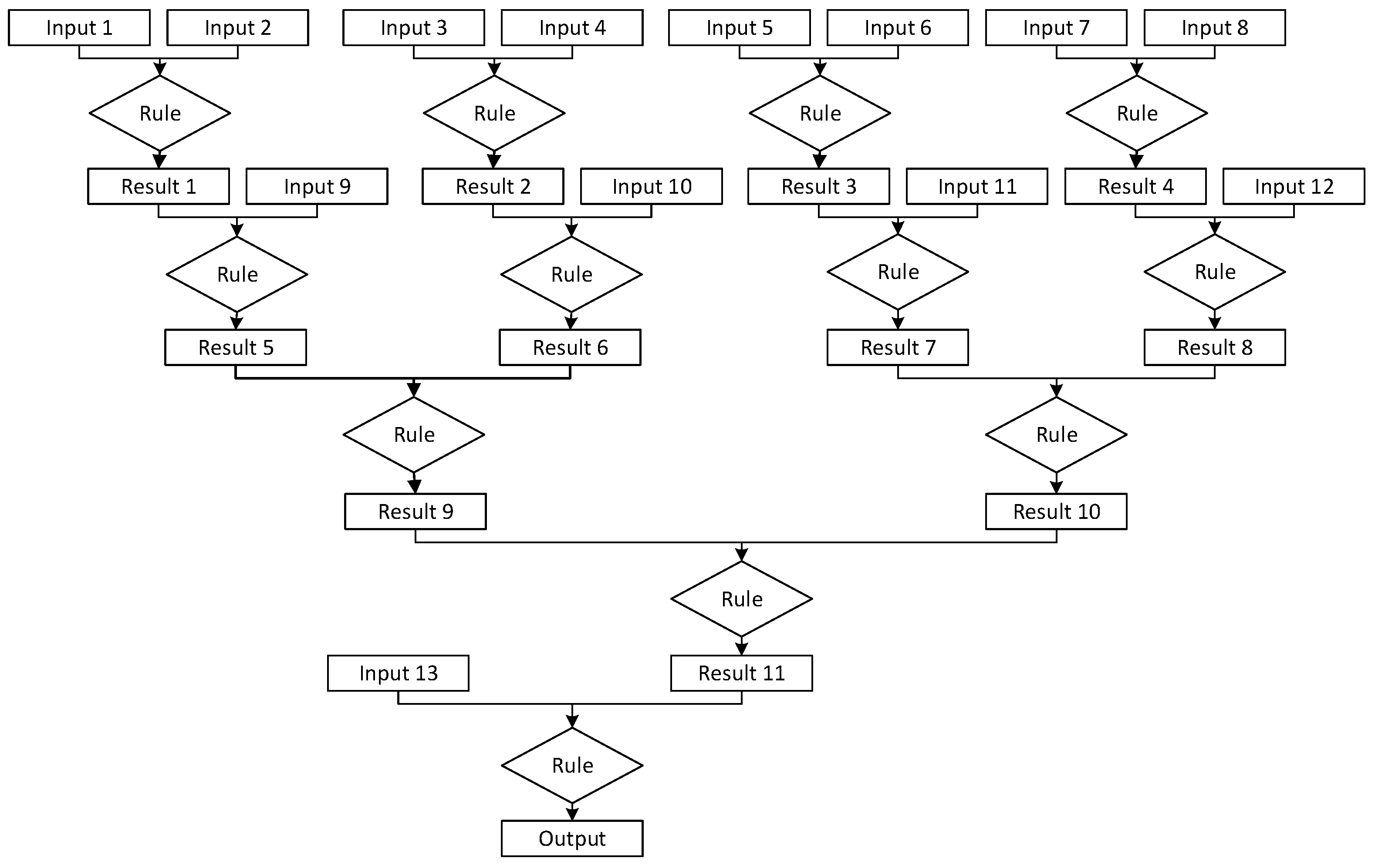
Figure 5 are distinct logical designs of rule-fact networks that were used to create both hardware and software expert systems for comparison purposes. These networks were designed to simulate how a real-world application of an expert system would work. Each has a different number of inputs and operations that work to produce a single output.
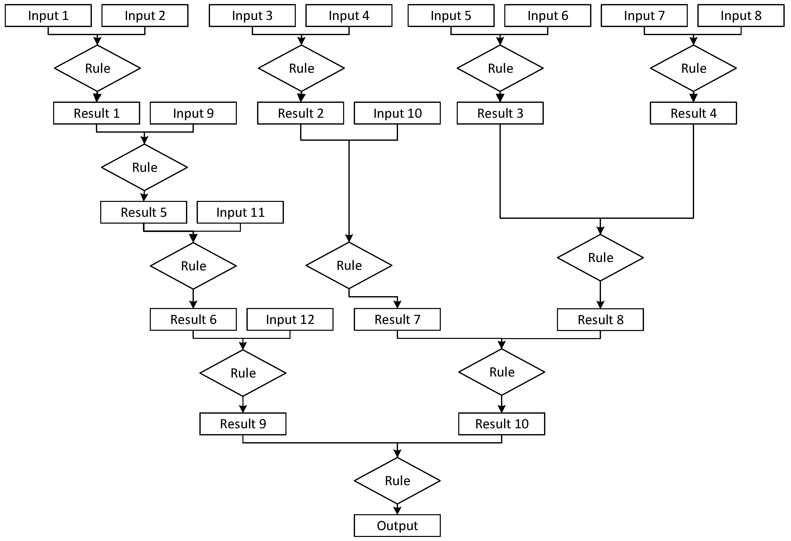
Network 1, for example, is a network that has an initial level of eight inputs and a second level of four additional inputs paired with the previous layers’ results. Then, the network requires an additional input on each layer up until the last layer to get a result. This network was designed to have characteristics in between those of a breadth-heavy and a depth-heavy network. It is slightly deeper than wide, with five rules in the completion path and the largest layer having four rules. A potential use case of Network 1 could be in a credit approval system that comes to a conclusion based off of many initial questions with some smaller additional follow-up data being used. Network 1 is shown in
Figure 1.
Network 2 was designed similarly to Network 1 but presents a scenario where, after the first and second layers requiring input, the network continues its processing without needing any additional input for two layers and then requires a final input before making its recommendation. As with Network 1, this network was designed to have characteristics in between the two extremes of high-width and high-depth networks. Its key focus was having most inputs supplied early in the network’s runtime.
Network 2 could be used within an application, such as identity verification, as most of the information is gathered at the beginning of the network with minor additional input or information being gathered later. The final input, number 13, would be typical of data that might be collected as part of a final validation step. Network 2 is depicted in
Figure 2.
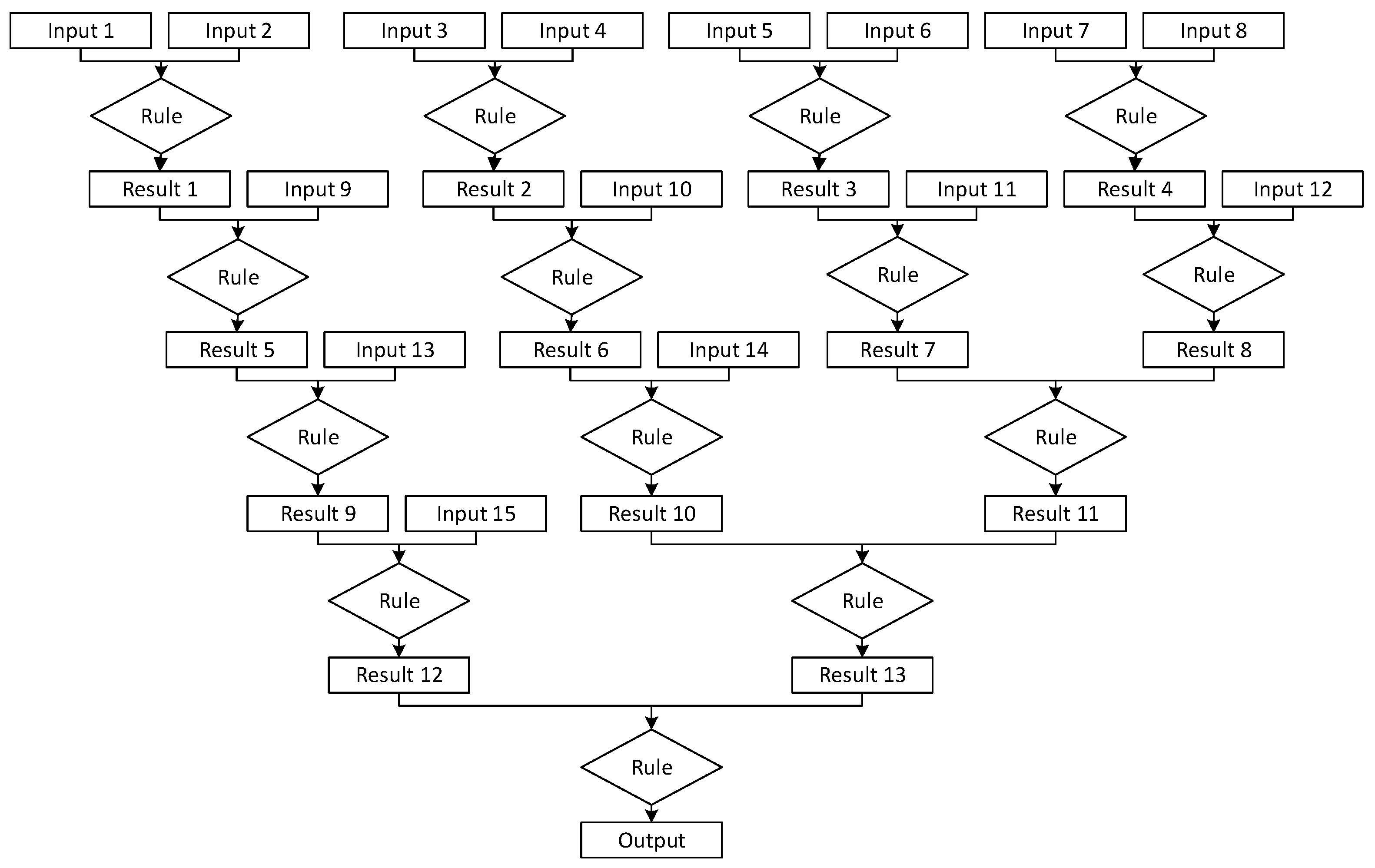
Network 3 was designed for a scenario that requires additional input paired with results from prior layers several times to draw a conclusion. This network was designed to be depth focused. It also incorporates inputs throughout this depth, as each layer requires additional information prior to the final two resulting facts being processed by a final rule to generate the recommendation or decision. Network 3 could serve very well in troubleshooting applications where, following the initial inputs, additional data are needed based on the information previously provided. Network 3 is presented in
Figure 3.
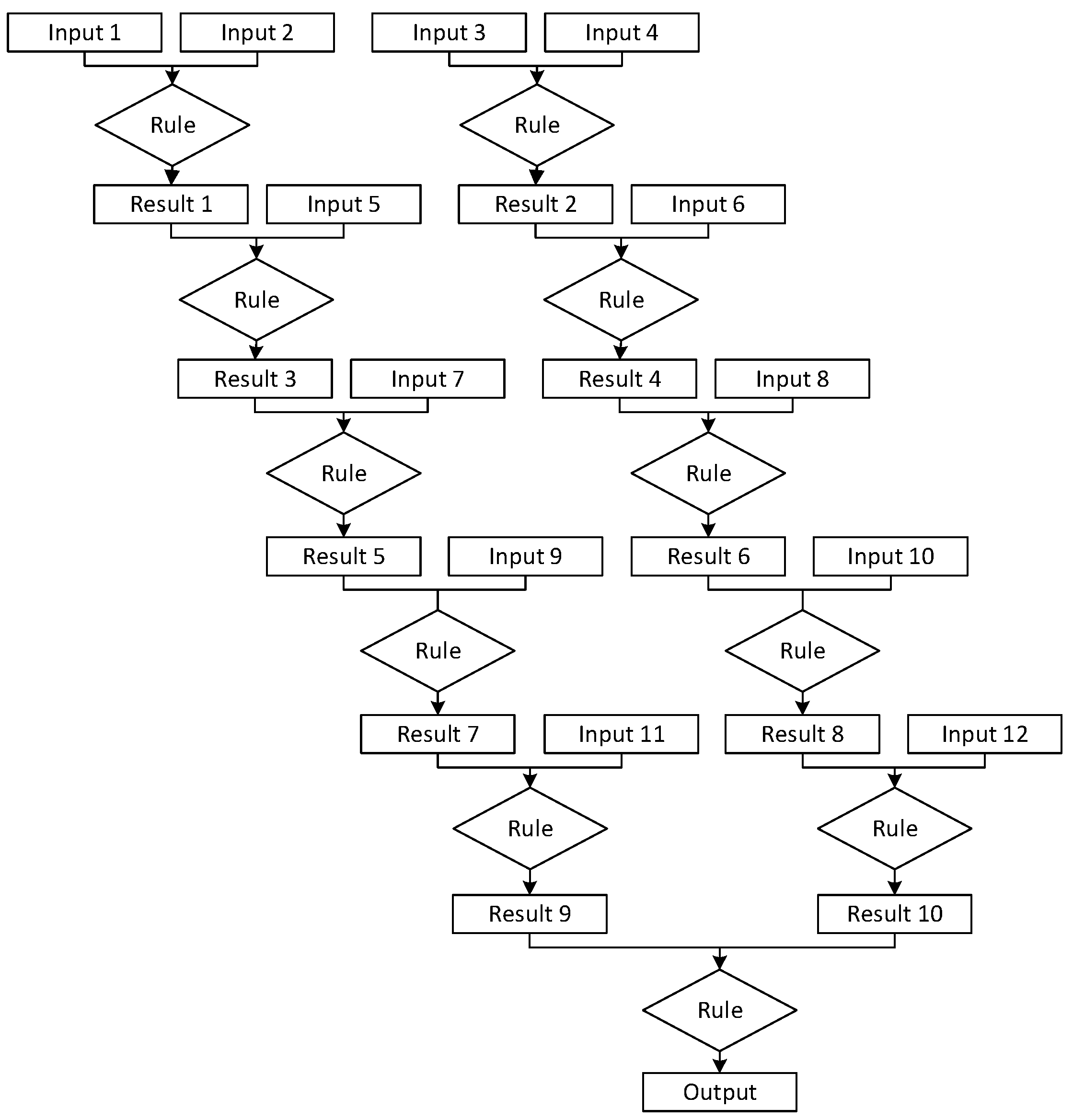
Network 4 shares the same structure as Network 2 but adds an initial layer in which four inputs are initially required, and their result replaces two initial inputs in the following iteration. This network was designed to be a breadth-heavy network whose inputs are supplied early in network operations, leaving about half of the layers to operate without requiring any additional inputs. While the network has a lot more breadth than Network 3, Network 4 could also find use in troubleshooting applications that, after an initial iteration where a problem is identified, need additional preliminary information in the next layer, with additional follow-up data being needed throughout the rest of the network. Network 4 is shown in
Figure 4.
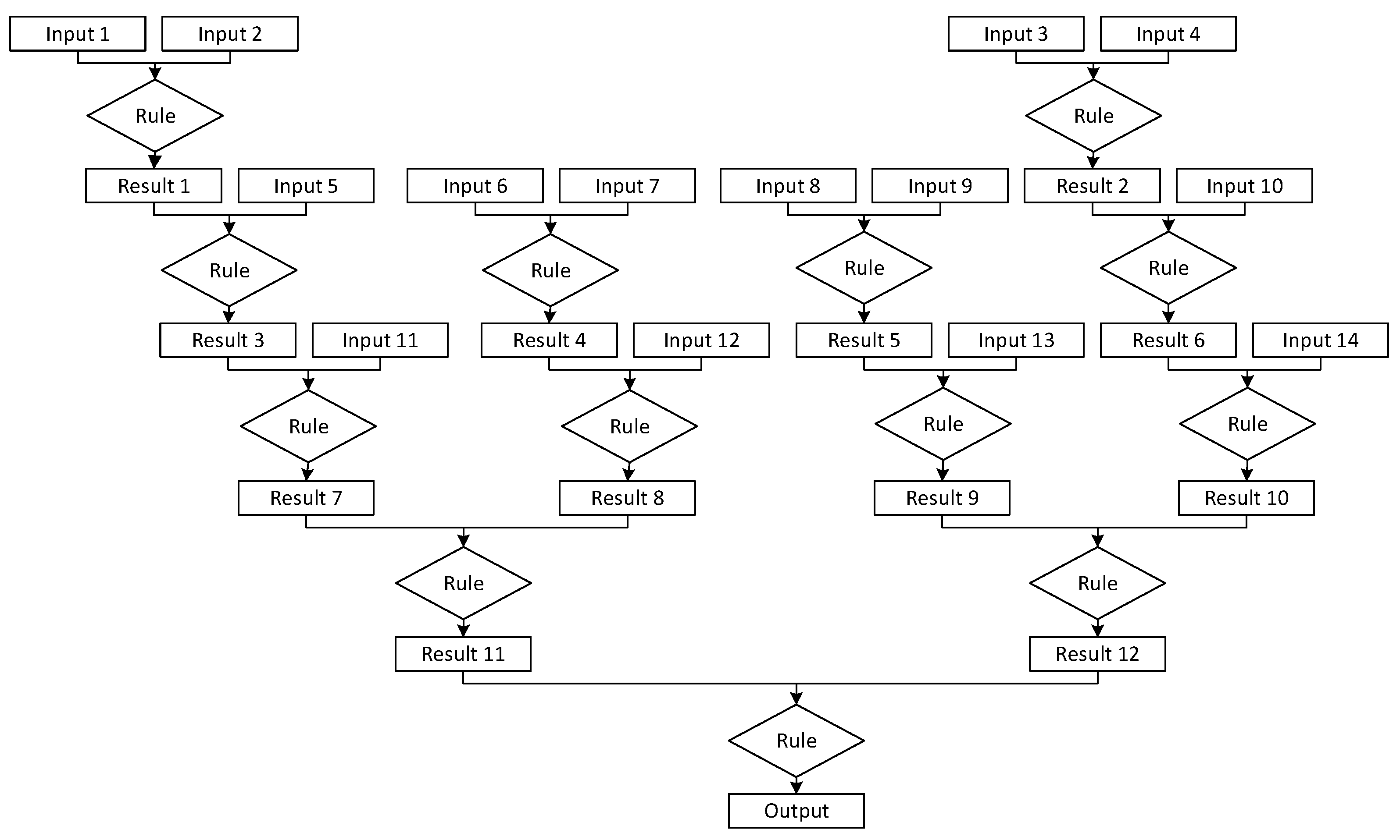
Finally, Network 5 is designed for a scenario that, after the initial layer’s inputs, has a combination of paths that require multiple inputs later in the process and paths that require no further inputs. This network was designed to fall in between the breadth and depth-heavy designs and requires several inputs for each layer in the first half of the network. It also, notably, has some facts that bypass network layers, being generated in an earlier layer and maintained for later use. Network 5 could be appropriate for use by a process control application with various preferences and settings. Some settings trigger a need for additional configuration parameters, while others do not. Network 5 is presented in
Figure 5.
The five different designs of networks were created to assess what the expected runtimes would be for different applications and their applicable network designs. This analysis can also be used to project how runtimes might increase for similar designs of networks at a larger scale. Networks 1, 2 and 5 were designed with more of a focus on the breadth of the network, to showcase different potential designs for applications that would require many additional inputs. Networks 3 and 4 were designed to show what a network that has more of a focus on depth than on the network breadth would look like and how it would operate. A feature that is shared by all of the networks is that, for the initial iteration, they all require inputs into both sides of the gates. This is a requirement as the first iteration is the entry point into the network and is not a continuation off a different network.
The main consideration when designing the networks was to use different internal structures along with differing amounts of inputs and gates to gather data on what runtimes would be. These data can inform the design and predict the time cost when creating larger networks.
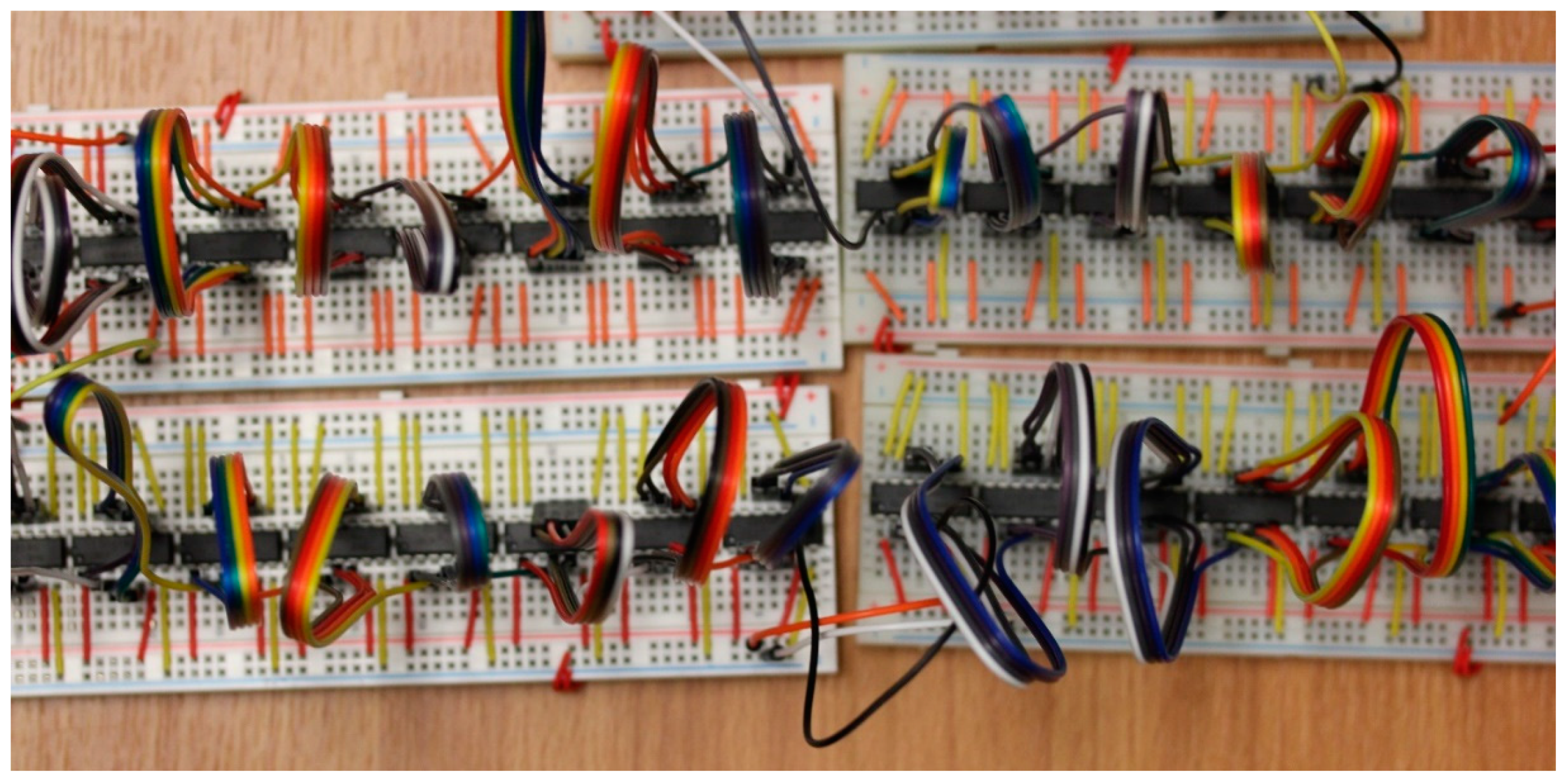
3.2. Hardware Design
Hardware-based networks were designed and built using breadboards that each included eight Texas Instruments CD4081BE AND-gate chips. Each of these chips contains four AND-gates, making a total of 32 gates per board.
Using these boards, two different types of networks were created, as described previously. First, deep networks were created for speed testing. For these networks, each gate had a single hard-coded input and an input that came from a previous gate. This was performed to test the propagation time of a single signal through the entire network. This system, thus, did not require all of the inputs which would be required for a large network to be set by a microcontroller. Instead, for testing purposes, a single input was sent that was passed through different numbers of gates, based on the experimental condition.
Second, the networks described in
Section 3.1 were built based on their logical diagrams. These networks were similar to the deep ones; however, instead of hard-coded inputs being used, every individual input signal that the network required was supplied by the microcontroller at runtime.
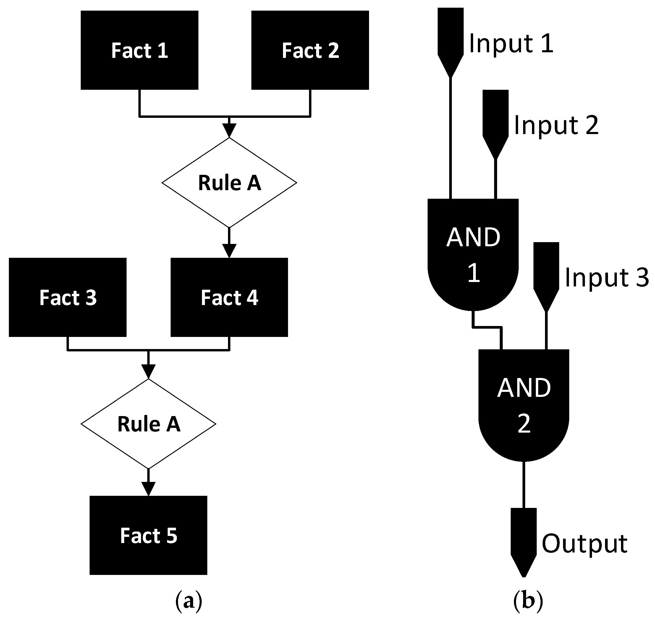
Figure 6 depicts how an expert system network (such as those presented in
Figure 1,
Figure 2,
Figure 3,
Figure 4 and
Figure 5) can be implemented into both software (
Figure 6a) and hardware (
Figure 6b).
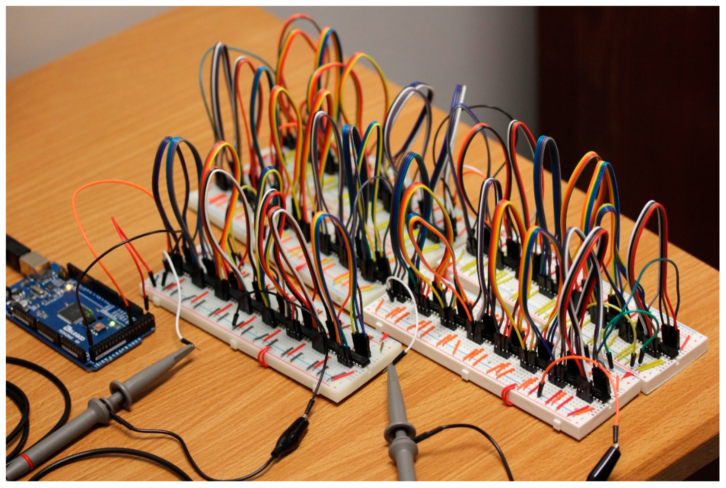
3.3. Experimental Setup
The experiment was comprised of two configurations. The first was for the deep network test and the second was for the real-world-based networks. For both tests, an Elegoo MEGA2560 R3 microcontroller was used to send inputs to the AND-gate network and a Hantek DSO5072P oscilloscope was used to receive a copy of the initial signal and the output, to time the operations of the hardware implementation. This configuration is depicted in
Figure A3. The second experiment also included a software-based expert system. The software-based expert system was run on a computer with an Intel Core i5-1135G7 processor, a base clock speed of 2.40 GHZ and 32 GB of 3200 MHZ DDR4 memory.
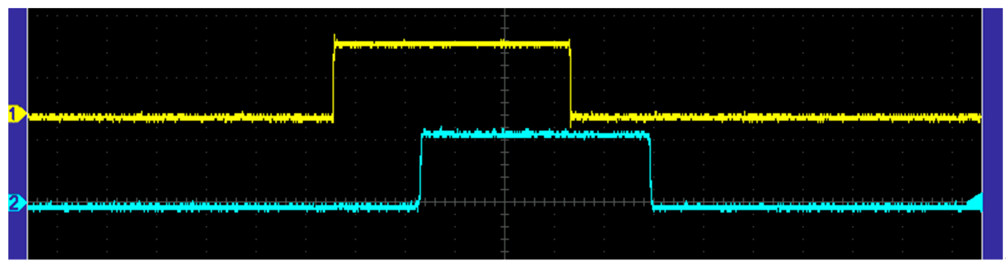
For the first experimental setup (the deep networks), a signal that alternated between digital zero and one (high and low) was sent by the microcontroller. The initial probe, connected to the oscilloscope, was used to measure when the first input into the network was sent, (i.e., when digital one/high was sent) with the microcontroller alternating between the high and a low signal. A second probe was attached to the final gate in the network—the output. Using the two probes and the oscilloscope, the time between the high signal from the first probe and the high signal from the second probe was recorded. This represents the signal propagation time across the network (i.e., the time it takes from when the initial probe reads a high signal to when the secondary probe reads the high signal). These propagation times were recorded and used to compare the time that it takes a signal to travel through networks with 32 to 160 gates. The signal propagation delay (the difference between the rise of the first and second channel) is shown in
Figure 7.
For the second experimental setup, the real-world-based networks, the probes were attached in the same manner. The difference between the two network designs was that in the real-world-based networks, many different inputs were required, rather than just the single input used in the large network tests. These were supplied by the microcontroller. For the timing of these networks, the initial probe was attached to the first input sent by the microcontroller, to take into consideration the additional processing time required by the network when the network is waiting for additional inputs from the microcontroller. The second probe was again attached to the final output gate of the network. Again, the propagation times were measured and compared (in the same way as described for the deep networks).
4. Data and Analysis
The two different experiments and their corresponding network designs were used to collect two types of data. The deep networks were used to collect data for five different network depth sizes. This was achieved by sending the signal through five subnetworks that each had 32 individual gates that the signal passes through. Results were gathered for 32, 64, 96, 128 and 160 gates by connecting one, two, three, four and five of the subnetworks together (in sequence).
For the smaller networks that were presented in
Section 3.1, each network was built in the same fashion as the deep networks (as described in
Section 3). For these network configurations, a software expert system (custom software written in C#) was also used, with the same network, to provide the computation time needed for computer-based processing of the network. This was compared to the hardware-based approach’s completion time.
For the hardware networks, timing was performed with an oscilloscope (as discussed in
Section 3) that was used to measure the delay in signal rise between the initial signal and the output signal of the networks. The software expert system was measured using a time function that is built into the Microsoft. Net framework.
4.1. Deep Network Propagation Experiment
For the deep network propagation experiment, interchanging high and low input signals were generated using a microcontroller at regular intervals, as previously discussed. This generated a block waveform which was measured to compare the initial rise of the network from a high input and the rise of the network’s output signal (i.e., the signal that had propagated through the network). For each network size (32, 64, 96, 128 and 160 gates), 25 tests were performed. The average, median, standard deviation and the minimum and maximum of the times for each set of runs are presented in
Table 1. For purposes of comparison, data were also gathered on the performance of the network with the gates in an unpowered state (while this resulted in unconventional behavior and would not be suitable for operational use, it does show the impact of the gates’ operation on system speed). These data are presented in
Table 2. After the network size tests were run, the time between the processing times of the networks and the number of individual gates were used to calculate an average processing time per gate in each network size. This is shown in
Table 3.
In addition to calculating the speed of the gates, another goal of this experiment was to ascertain if a loss of signal (voltage) would limit the number of gates that could be placed in series. This would inherently limit the size of the network and be a key design factor (as networks could potentially be designed to reduce the number of gates in series through the creation of parallel processing branches and other structural decisions. No notable level of signal loss was detected during this experiment. Thus, there is no evidence, at present, of a signal loss-based limitation on network size. Notably, parallel processing branches may also provide speed benefits (as gates operate truly in parallel), so this technique may still be used for this purpose, despite not being needed to overcome a signal loss-driven network length limitation.
4.2. Real-World-Based Network Model
For the real-world-based network experiment, similarly to the previous experiment, a high and low input signal were generated using the microcontroller. Signal propagation (based on receiving the correct output signal) was measured from the start of the first input to the final output signal. For each network, 10 tests were performed and the average, median, standard deviation, minimum and maximum were calculated. The results of the hardware-based networks are presented in
Table 4. Notably, the networks produced the correct output consistently. This was assessed by visually inspecting the output waveform. If the network produced an incorrect result, the waveform would have a notable deviation in it. No such deviations were detected.
Additionally, the same network that was implemented using hardware gates was also implemented in software. The results from the software runs are presented in
Table 5. As with the hardware networks, the average, median, standard deviation, minimum and maximum are included.
For the real-world-based networks, there are two main design categories which have been implemented: wider networks and deeper networks. Wider networks, such as Networks 1, 2 and 5, would be applicable to applications that make decisions based on limited processing of a collection of initial given parameters. For example, an application for credit might draw upon a number of initial inputs (such as the applicant’s income, credit history, job history, etc.). However, once these inputs are known, the decision can be arrived at quickly—and most inputs are used in most decisions (as opposed to deeper networks with later-used inputs which thus draw upon additional data in some, but not all, circumstances).
Networks 3 and 4, on the other hand, utilize more depth. Network 3 is the most depth focused while Network 4 falls in between the depth of Network 3 and the lower depth levels of Networks 1, 2 and 5. Network 3 would be representative of troubleshooting-type applications (such as computer support or medical diagnosis) where there are a small number of initial inputs or questions; however, throughout the process additional input may be required to reach a conclusion.
Due to falling in between the depth-focused Network 5 and the other shallower networks, Network 4 would be representative of a more complex troubleshooting setup. This could involve a smaller number of initial questions, some of which trigger a need for additional data to support decision/recommendation making.
4.3. Analysis
For the signal propagation time experiment, as expected, when additional gates were added to the overall network, the time for the signal to propagate (and thus the network to process) increased nearly linearly. There was, however, a slight difference between the additional time cost of 128 gates and 160 gates which may be attributable to production irregularities of the gates or the result of other similar causes.
On average, for each additional 32 gates there was roughly an increase of 1.1 μs of processing time above the base 1.2 μs propagation time with only 32 gates in the network. The data regarding the speed of signal propagation provide a basis for modeling an expert-system that can make decisions at a much faster speed than a computer-based one. This could prove beneficial in applications where a system’s speed is important. Notably, the gates still take more time to operate than current flow without them, as the signal propagation speed increases to be roughly 30 times as fast through a set of gates that are not powered. This demonstrates the notable difference in speed at which the signal flows through the gates when they are not making any logical calculations and are simply providing a conduit.
For the real-world-based networks, the logical networks shown in
Figure 1,
Figure 2,
Figure 3,
Figure 4 and
Figure 5 were created in both hardware-based and software based expert systems. As shown in
Table 4, each of the software-based networks ran the network at a speed between 2.4 and 6.8 ms, with an average for each network being between 4.4 and 4.9 ms. Notably, the timing of the networks did not include the creation of the network and only included the processing of the network to facilitate direct comparison with the hardware-based expert system’s performance.
The hardware-based networks, on the other hand, took between 0.04 ms and 0.05 ms, on average, to run. This means that, for each network, the hardware-based expert system ran approximately 95 times faster than the software version. While the difference in timing between the hardware and software networks is significant, it is also notable that the real-world-based networks operate significantly slower than the large deep network tests, where a single signal propagates through a network, despite being smaller. Each of the large deep networks has between 32 to 160 gates, whereas the real-world-based networks have between 10 and 14 gates. This speed difference is largely due to the processing speed of the microcontroller that sends the input signals. The microcontroller can only set one signal at a time and the signal propagates through the network of gates significantly faster than the controller is able to provide all the input signals to the network. Practically, this means that large and complex networks will have a performance that is quite similar to smaller networks, as long as they have a similar number of inputs supplied by a microcontroller of this speed.
This also means that the performance of the system could be demonstrably enhanced by supplying different values from multiple microcontrollers or a faster microcontroller. Prospectively, the gate-based system could be supplied directly from sensors and other data sources in robotic systems, facilitating the maximum use of the gate network’s processing speed.
In
Table 3, the processing time per gate was calculated for each of the large deep network configurations. It ranged between 34.5 and 39.7 ns. The input time, on the other hand, was measured to be 3.945 ± 0.005 μs per gate input. This means that the per-gate processing time is approximately 100 times smaller than the input time. This comparatively small amount of processing time means that, for real-world applications using a hardware-based system, the network processing time is dwarfed by the time required for input processing for the number of inputs that are provided to the network. Practically, this means that anything that can be calculated from an input (or a combination of inputs) should be arrived at this way, to save loading time. It also suggests that there is a limited time cost when designing more robust rule-fact networks which use a larger number of rules to perform more detailed analysis for hardware expert systems. This is a significant difference as compared to software-based expert systems which incur significant time costs with the rule selection and processing steps. Additionally, software-based expert systems must save their results to intermediate facts while intermediate values are carried by wire directly to their next rule in the hardware-based expert systems.
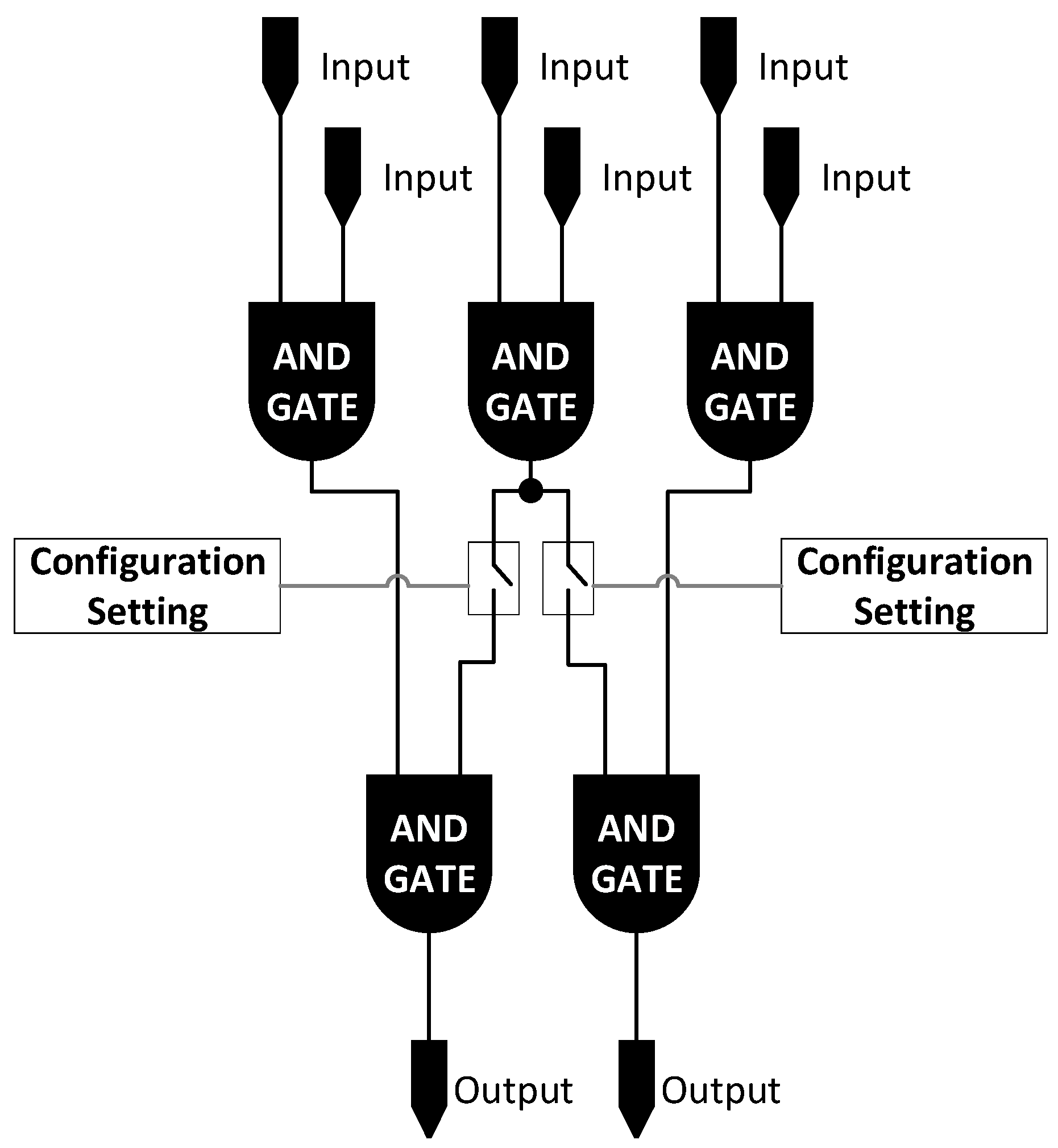
Based upon the analysis conducted and the efficiencies identified, an expert system hardware module could be used to expedite processing. This type of hardware module could have a collection of pre-interlinked gates with the capability to turn connections off to match the logical system design. A large, highly connected network could be built. This would then be reduced to the specific configuration of a given network via configuration options which would be used to set flip-flop (set/reset) components to disable pathways between gates which are not present in the network design. This concept is depicted in
Figure 8.
4.4. Real World Operational Implications
A variety of real-world operational benefits are presented by the enhanced performance of the hardware expert systems. In a batch processing environment, the two orders-of-magnitude performance enhancement would allow approximately 100 decisions to be made in the time normally taken by one. This facilitates more processing being performed by the same number of systems or can reduce the number of systems needed. This benefit is further enhanced by the likely lower cost levels of the hardware expert system compared to a full-fledged computer.
The benefit can also be considered in terms of robot response impact.
Table 6 and
Table 7 present this benefit.
Table 6 shows the hardware and software time requirements for each of the five test networks and the time savings enjoyed by using the hardware system.
Table 7 assesses what the difference level for Network 1 (given the similarities in difference levels for the five networks, the other networks’ results would be similar to Network 1’s) would mean in terms of saved travel distance and extra maneuverability. Notably, for orbital vehicles and HTV-2 aircraft, the time savings provides 4 and 3 m of maneuverability, respectively. This additional capability could potentially be critical in collision avoidance from another satellite or aircraft crossing one of these vehicles’ paths.
While the five networks presented may have the complexity of an automated collision avoidance system, route selection and planning systems would be inherently more complex. The enhanced hardware expert system performance thus might allow a more robust planning decision-making process to be made in the same time that only a basic avoidance process could run on a software expert system. This would facilitate better decisions which not only avoid the obstacle but also chose a more path-resumption-optimal means of doing so.
Beyond emergency response, the processing time reduction can facilitate evaluating a greater number of potential options for a decision, leading to potentially better decision-making. It may also facilitate decision-making systems being run, to update mid-range and long-term plans, more frequently. Thus, the proposed hardware expert system implementation approach provides a logic-capability-rich reflex arc [
78] style function (facilitating fast response without core command system involvement) while also being useful for larger-scale decision-making and planning processes.
5. Comparison to Other Techniques
Several different classes of rule-fact expert system implementations exist. The most basic is the iterative expert system, where rules are selected to run each iteration and then run with the cycle repeating until no rules remain (or some other termination condition exists). Predictive expert systems, such as the different Rete versions [
26,
79], do not run every rule. Instead, they select rules to run. These systems can run much faster due to this; however, many are proprietary and not available for direct comparison to new systems. Neural networks have found uses similar to expert systems and offer a training capability, in addition to decision or recommendation making. Finally, hardware expert systems are described herein. Notably, hybrid systems are possible, as the use of neural networks for developing expert system networks [
80] and the use of gradient descent techniques for training expert systems [
32] have been proposed.
Table 8 compares these forms of expert systems in terms of six metrics. Understandability is a measure of how easily the decisions that the system makes can be understood in terms of what caused them. Systems with high traceability perform well in terms of this metric, while systems that cannot track their decision-making back to specific causes do not perform as well. Neural networks, in this area, suffer from the potential that learning-caused changes may change the decision arrived at from a single set of inputs on a regular (or continuous) basis. Predictive expert systems largely have proprietary engines, making it difficult to understand their specific outcomes.
Defensibility presents similar considerations—however, the question here goes beyond just whether a system’s decisions can be understood after the fact to whether a system will always give a similar answer with a similar set of inputs. Again, the potential for training-caused changes in neural networks impairs their performance in terms of this metric. The fact that different outputs can result from different rule selection orders, under the iterative and predictive expert systems, impairs their performance in terms of this metric.
The speed of the systems is then compared. Notably, the predictive and hardware expert systems outperform the other types. This is explained by the factor that causes time growth, which is also included, for each, in the table.
Reproducibility is highly linked to defensibility. It is a metric of whether the same experiment run on the same network would yield the same results. Again, neural networks training and predictive expert systems’ rule selection ambiguity impact their performance in terms of this metric.
Finally, changeability is the last key metric. Neural networks perform very well in terms of this metric, due to their self-learning mechanisms. Iterative and predictive systems are, similarly, easily changed by changing their network structure in memory or storage on the processing system (without requiring coding changes, in many cases). Hardware expert systems may be unchangeable (if implemented on a printed circuit board) or expensive to change, due to the need to reconfigure the hardware to the new network design.
6. Conclusions
This paper has described how a hardware-based expert system can be created using logical AND gates and a basic microcontroller. It has discussed several prospective applications of hardware-based expert systems and how they could improve over current software-based expert systems for some applications. The use of hardware for expert system implementation allows much faster network processing. The level of enhanced speed has been quantified herein as being approximately 95 times as fast. This enhanced speed provides significant benefit for applications, such as robotics, where decision-making needs to happen quickly. Additionally, as the data show, there is minimal variation. Thus, hardware-based expert systems also benefit applications that need to make decisions within a constrained amount of time. For some applications, software-based implementation may lack the processing speed required. In other cases, a more expensive computer could be replaced by a less expensive hardware-based expert system which also provides speed-enhancement benefits.
For robotics, autonomous machinery and other similar applications, such as self-driving vehicles and artificial intelligence-operated robots or drones, the hardware-based expert system approach to decision making may be of particular utility. While some applications are fine relying on software-based control systems (for example, applications that that are not making real-time decisions), others will require rapid decision-making and decision-making within a known and constrained period of time. Robots, for example, must be able to make a decision within their obstacle-sensing timeframe (the time between when an object is sensed and when the robot would arrive at the object’s position).
Utilizing a hardware-based expert system implementation eliminates some processing time and allows for rapid processing capabilities, once all inputs are supplied to the network. As inputs could potentially be supplied directly by sensors, even this may not be a significant time constraint for some robotic systems. This is well-suited for systems that need nearly instantaneous decision-making capabilities. An autonomous drone’s fast decision-making, for example, could provide the difference between the drone being able to maneuver around a moving obstacle or being unable to respond quickly enough to avoid it and crashing.
In addition to removing limits on the potential performance that a network may be capable of delivering, hardware-based implementations may facilitate placing certain systems (such as obstacle avoidance) closer to sensing or control systems (as opposed to these being in a central processing location). This proximality may also offer additional speed of response benefits.
This low-cost logical processing capability may also be well suited to enable a variety of other applications. For example, it could be used to build an autonomous troubleshooting capability into large machinery. Without requiring the cost of a computer (and the wear-and-tear considerations of hard drives, fans and other parts), a system could be included that would facilitate troubleshooting the device and going through steps required to return to an operational state, without requiring a field support technician to go and visit it to troubleshoot it. Autonomous troubleshooting could be connected to key systems throughout the machine and, when self-diagnosis detects that the machine is not fully operational, it could begin its autonomous troubleshooting to attempt to return the device to an operational state. If this fails, it could also perform preliminary analysis to ensure that any technician deployed to service it has the appropriate skillset for the type of problem that has been detected. The low cost of this type of computing system facilitates its use as an add-on to other systems, without increasing their costs to the extent that an onboard computer system would.
In addition to the results described above, this work has identified a number of areas for future exploration. Planned future work includes assessing different approaches to reduce or eliminate the time cost incurred by the microcontroller loading of fact data. It will also include developing larger network examples to further test the effectiveness of using a hardware-based approach to developing an expert system for specific applications and the evaluation of the use of customizable AND-gate networks.


