Abstract
The automotive industry is undergoing a transformational period where more and more new energy vehicles (NEVs) are being produced and delivered to the market. Accordingly, some new challenges arise during the manufacturing process for car companies. Since the mixed-model assembly line has been widely used, how to integrate the NEVs into the existing assembly system that was designed for the production of gasoline cars is a key issue. A practical approach assigning a specific workforce to handle NEV assembly work is applied at the BMW assembly shop. This work studies this new production pattern and focuses on the design of the assembly system under this pattern. This work aims to develop a method for minimizing the production cost of NEV assembly. Thus, an exact algorithm for hierarchically solving the assembly line balancing problem and vehicle model sequencing problem is proposed. Mixed integer programming mathematical models that describe these two problems are formulated for the first time. Three new benchmark problems and one industry case that include the NEV models are created to evaluate the effectiveness of the proposed method. Results of numerical tests demonstrate that the developed algorithm can quickly generate reconfiguration solutions of the assembly line for various model mix scenarios and production rates. High flexibility of the manufacturing system can be obtained using the proposed approach.
1. Introduction
Sales of New Energy Vehicles (NEVs) have been continuously increasing around the global automotive market in the recent decade. NEVs, such as the battery electric vehicle (BEV) and plug-in hybrid electric vehicle (PHEV), have been mass-produced by many automotive companies. At the assembly production phase, most automotive manufactures produce multi-models in one assembly line to minimize the production cost. Integrating the NEVs into the existing assembly line is a cost-efficient way to realize NEV assembly production. The NEV has a lot of unique parts due to the architectural differences between NEVs and conventional gasoline cars. These differences require additional equipment, tools, operations and workers on the assembly line. Since the assembly line is a paced system where all workstations and workers operate under a fixed cycle time, integration of the production of NEVs will cause fluctuations to the existing assembly system. An inappropriate schedule can either result in shutting down due to the limitation of production capabilities or the wastage of production resources. Consequently, a practical approach adopted at the original equipment manufacturer (OEM) involves arranging a group of people responsible for the assembly of NEVs. These people, who are the supplementary labor force, are only involved in the installation of NEV-specific parts. As a result, in this way the disturbance in the assembly system caused by the integration of the NEVs can be minimized.
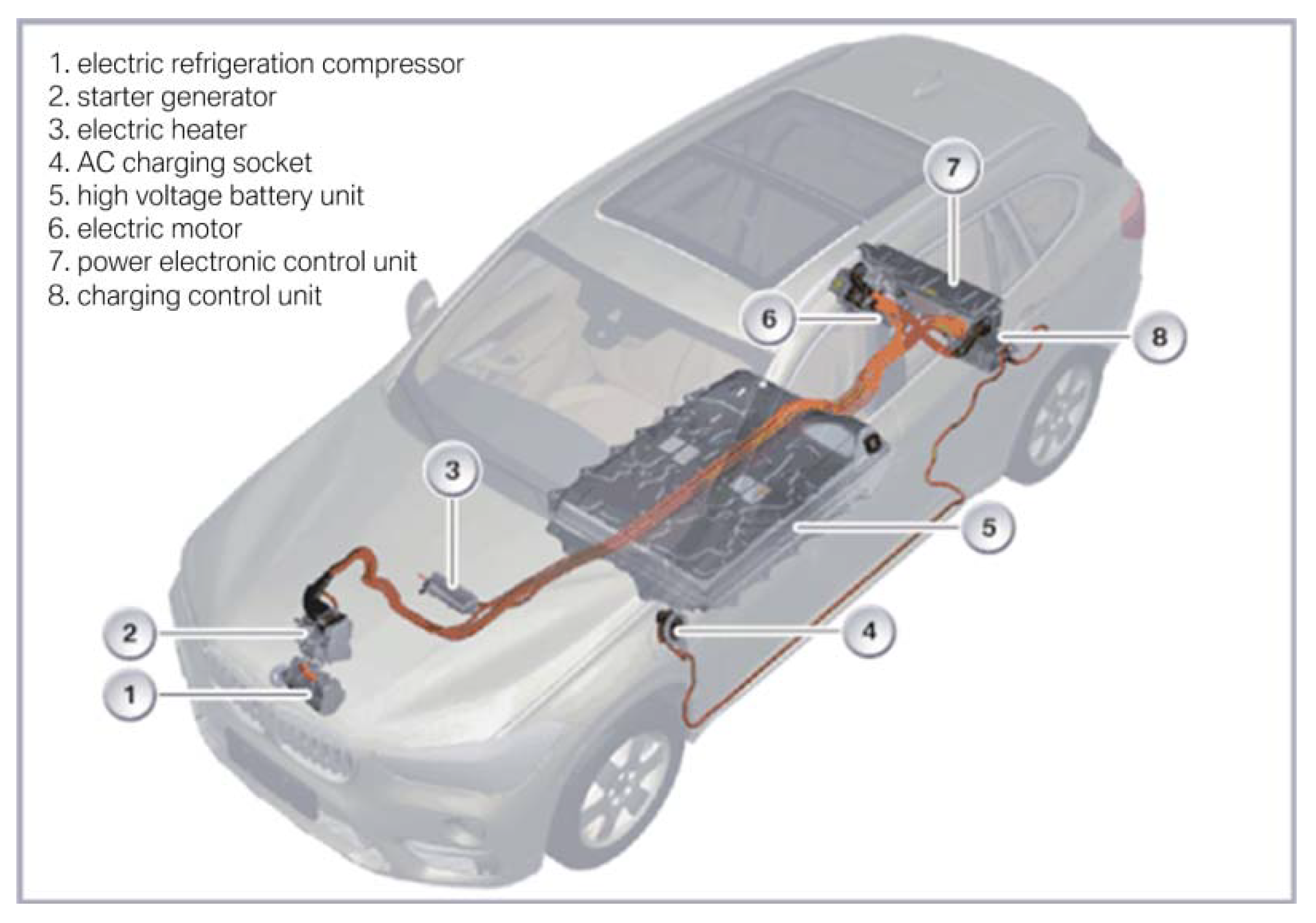
Mixed-model assembly lines are commonly used to produce various models that belong to the same product segment and different configurations of one model. These vehicles have a feature that their main structures are similar. Thus, the difference of assembly processes among different models is not significant [1]. A lot of stand tools and equipment can be shared for the mixed-model assembly production. However, assembling components of the NEVs’ electrical system, which contains the battery module, high voltage cables, electric motors, and power electronic devices, needs specific processes. When bringing the NEV into an existing assembly line, the original production scheme can hardly handle these additional operations through simple adjustments. For example, to integrate the BMW X1 PHEV into BMW Tiexi Assembly shop, more than 80 new tasks related to the high voltage components (highlighted in Figure 1) need to be accomplished. As a result, twelve new added operators are assigned to the main assembly line. These people, also called PHEV workers, are specifically responsible for the X1 PHEV model. They act as a supplementary workforce to complete the assembly production together with the normal operators. Different from the traditional production pattern where workers operate within a fixed workstation area, a PHEV worker can follow the car across several workstations until he/she finishes the assigned assembly tasks. This production pattern with floating PHEV workers along the assembly line is called ‘floating pattern’ in this study.
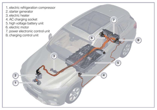
Figure 1.
High voltage components of the BMW X1 PHEV.
Assembly line balancing and vehicle sequencing are two main issues in mixed-model assembly line research. The assembly line balancing (ALB) problem involves searching for the optimum assignment of assembly tasks to workstations given precedence constraints according to a pre-defined single or multi-objective goal [1]. The sequencing problem aims to minimize the line starvation and/or congestion through scheduling the model sequence according to which vehicles are released into the production line [2]. The production sequence of vehicles is also proved to obviously influence the utilization and production efficiency in the mixed-model assembly line. In this work we focus on the Mixed-model Assembly Line Balancing Problem under the Floating pattern (MALBP_F) and Vehicle Sequencing Problem (VSP) of the NEV assembly production.
The major contributions of this paper are: (1) According to our best knowledge, it is the first time the mixed-model assembly production with the NEVs has been systematically studied. Two main problems, which are the MALBP_F and the VSP, are investigated in this work to minimize the number of workstations and total workers. (2) A hierarchical computing procedure is developed to solve the MALBP_F and VSP. Mathematical models of these problems are formulated. (3) Three benchmark problems and one real production case are presented to test the performance of our proposed approach. The experiment results demonstrate that the proposed method can be efficiently applied to two common situations in the automotive assembly production: First, production rate increases, which result in shorter cycle times; second, vehicle model mix changes in the production plan.
The structure of this article is as follows: (1) we introduce the industrial background of this research; (2) next review the studies on mixed-model assembly line balancing and sequencing problem; (3) we describe the MALBP_F and present the mixed-integer programming model of this problem; (4) we model the VSP and design a hierarchal procedure to solve the MALBP_F and VSP; (5) we conduct numerical experiments and analyze the results and (6) the conclusions of this work are presented.
2. Literature Review
Mixed-model assembly lines have been widely studied by many researchers. Comprehensive reviews of the study of line balancing problems are given by Battaia and Dolgui [3] and Eghtesadifard et al. [4]. Boysen et al. [5] presented a review of the sequencing issues of mixed-model assembly lines. Two basic problems are mainly studied for the mixed-model assembly system: the Mixed-model Assembly Line Balancing Problem (MALBP) and the VSP.
Some researchers focus on solving the MALBP and VSP separately. Simaria and Vilarinho [6] solved the problem of line balancing a mixed-model assembly line by using a genetic algorithm. They also tried to utilize an ant colony optimization algorithm to solve the line balancing problem with parallel workstations. Bukchin and Rabinowitch [7] proposed a branch-and-bound algorithm to minimize the number of stations and task duplication costs of the line balancing problem. Yagmahan [8] solved the MALBP considering the line efficiency, capacity utilization and discrepancies among station times. Manavizadeh et al. [9] proposed using the multi-objective evolutionary algorithm to resolve the line balancing problem of a mixed-model assembly line. Hyun et al. [10] studied the mixed-model sequencing problem with multiple objectives using the genetic algorithm. McMullen and Frazier [11] presented a simulated annealing approach to mixed-model sequencing problems. Ishigaki and Miyashita [12] developed algorithms for the sequencing problem in mixed-model assembly lines. Bautista et al. solved the mixed-model sequencing problem with work overload, useless time, and production mix restrictions [13,14].
Since the line balancing problem and model sequencing problem are tightly interrelated with each other in practical assembly production, these two problems are naturally dealt with when planning a mixed-model assembly line. One common approach is to solve the line balancing and sequencing problem hierarchically [15,16]. Hwang and Katayama [15] designed a hierarchical procedure for line balancing and model sequencing problems. Faccio et al. [16] studied mixed-model assembly line with jolly operators, and they proposed a hierarchical method to solve the line balancing and sequencing problem. An evolutionary algorithm is applied in their approach. Another approach is to tackle these two problems simultaneously. Kim et al. [17] adopted a coevolutionary algorithm to solve the line balancing and sequencing problems at the same time. Mosadegh et al. [18] presented a mixed-integer linear programming model to jointly solve the line balancing and sequencing problems. Saif et al. [19] applied a multi-objective artificial bee colony algorithm to solve these two problems simultaneously. Manavizadeh et al. [20] investigated multi-objective line balancing and model sequencing problems of mixed-model assembly production. A heuristic algorithm is proposed to solve both balancing and sequencing problems simultaneously. Kucukkoc and Zhang [21] developed a hybrid ant colony optimization-genetic algorithm approach to address the problems of line balancing and model sequencing.
Besides the basic simple straight line, mixed-model assembly lines with specific configurations are handled by some researchers. Balancing and sequencing mixed-model U-lines are conducted by Kim et al. [22,23]. Rabbani et al. [24] studied the U-line balancing problem of type-I, they also investigated mixed-model assembly U-lines considering human-related issues [25]. Mosadegh et al. [26] extended their studies considering the station-dependent assembly times for mixed-model assembly lines. U-lines have some advantages compared to the traditional straight lines: (a) good visibility and communications among operators, (b) more flexibility with multiskilled operators, (c) quick rebalancing the line. However, U-lines have some limitations when producing new energy vehicles. A key characteristic of the U-lines is that the entrance and exit of U-lines are located at the same position. Since the main lines in automotive assembly shops usually have more than one hundred workstations (200+ at BMW), U-shaped lines are not applicable to the automotive assembly production. Besides, high voltage operation qualification is necessary for the installations of high voltage components on the NEVs; multiskilled operators on the U-lines means higher training cost compared to the floating pattern with specific PHEV workers. Mixed-model assembly lines with parallel workstations have been studied by Vilarinho and Simaria [27] and Rabbani et al. [28]. Kucukkoc and Zhang [29] applied an ant colony algorithm to solve line balancing problem for mixed-model parallel two-sided assembly lines. Akpinar and Baykasoglu [30] developed a mixed-integer linear programming model for the type-I MALBP. Their proposed model can deal with problems considering the sequence dependent setup times between tasks, parallel workstation assignments and zoning constraints. They also solved the problem with a multiple colony hybrid bee algorithm which is a meta-heuristic algorithm [31]. Zhao et al. [32] took the impact of mental workload into consideration as it can affect the product quality and efficiency. A mathematical model of multi-objective mixed-model assembly line balancing problem is formulated and a genetic algorithm is applied to solve it. Parallel workstations or parallel lines possess the flexibility of cycle time design and workstation arrangement. However, paralleling results in the additional workstation construction and equipment cost. Paralleling design can be realized in a new assembly shop at the early phase, but it is hard to transform a straight line into parallel lines. Thus, paralleling methods are not practical for integrating NEVs into the existing assembly line.
An assembly line allowing several workers to operate on the same workpiece, which is different from the traditional line configuration, is defined as a multi-manned assembly line. Dimitriadis [33] first studied the multi-manned assembly line balancing problem. He developed a heuristic algorithm to minimize the total number of workstations required. Becker and Scholl [34] generated a mixed integer programming model of the multi-manned assembly line balancing problem. Fattahi et al. [35] investigate the multi-manned assembly line balancing problem to minimize the number of workers. Yazdanparast and Hajihosseini [36] considered the same problem as [35]. They developed a mixed integer programming formulation based on the assumption that the task times are not deterministic and related to the number of workers. Kazemi and Sedighi [37] developed the mixed-model multi-manned assembly line balancing problem using a cost-oriented approach. They designed a genetic algorithm and a particle swarm optimization algorithm for solving the problem efficiently. Roshani and Nezami [38] addressed the multi-manned assembly line balancing problem to minimize the cycle time and the total number of workers. Kellegöz [39] continued the work of Kellegöz and Toklu [40] to solve two objectives of multi-manned assembly line balancing problem: minimization of both the total number of workers and the number of workstations.
It is clear from papers reviewed above that there is a lack of research on the mixed-model assembly production under the floating pattern. There has been no reported research that presents a detailed study of MALBP_F and VSP. These practical configurations that appeared during the process of manufacturing NEVs produce the basic motivation of this article. This work aims to present a novel framework of solving the MALBP_F and VSP exactly for the mixed-model production of NEVs.
3. Description and Modeling of MALBP_F
3.1. Problem Description
At the early phase after Start of Production (SOP) of the PHEV, sales and orders of this type of model are relatively small. Since the planned workforce must satisfy the requirement of the PHEV model which possesses the maximum workload, there will be a huge wastage of labor force if we balance the mixed-model assembly line using the traditional approach. Normally, operators are assigned to a fixed workstation within a relatively small working area on the assembly line. When the PHEV model ratio on the line is small, the new added workers will generate a considerable amount of idle time during the assembly of conventional gasoline cars. To minimize the fluctuation caused by the introduction of PHEVs, the floating pattern is applied to the mixed-model assembly line. PHEV workers, as the supplementary workforce, are the staff dedicated to install those extra parts on the PHEV under the floating pattern.
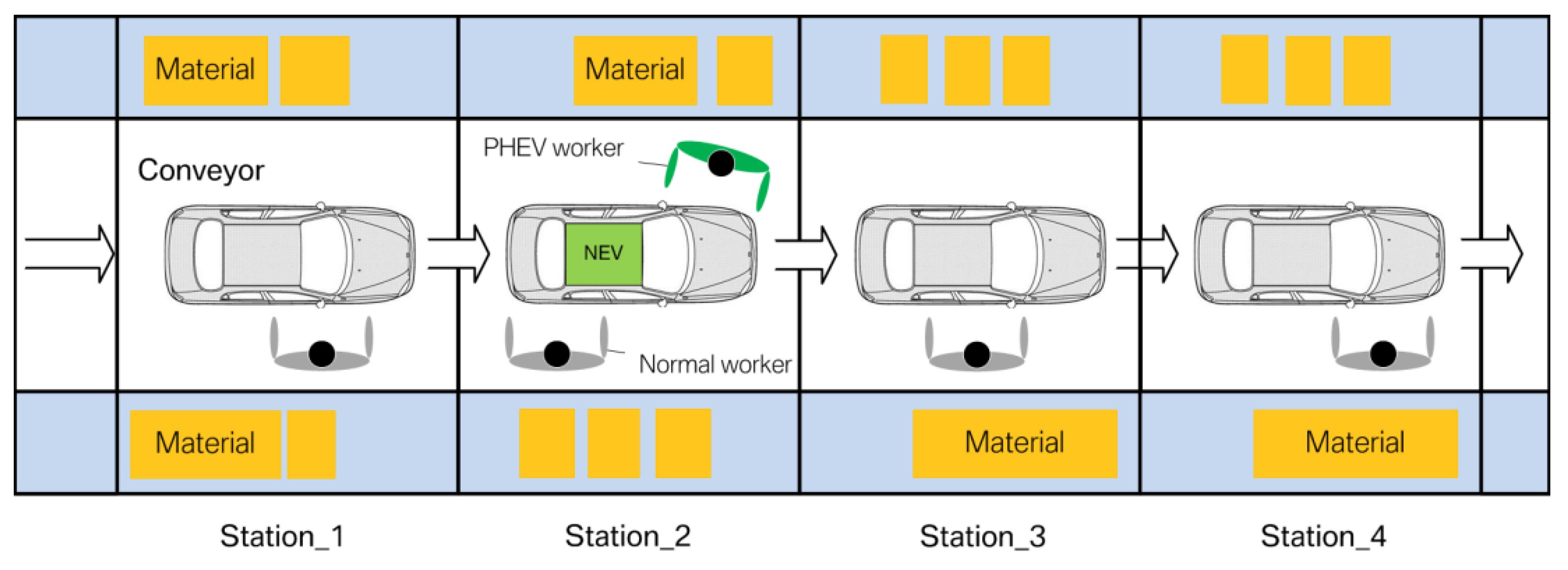
Figure 2 shows the mechanism of the floating pattern for the PHEV assembly. Two kinds of workforce are arranged in the assembly line: normal workers (grey ones) and PHEV workers (green one). As stated earlier, each normal worker belongs to one workstation and is only responsible for tasks assigned to that workstation. For the PHEV worker, the range of his/her working area should be predetermined. Usually, that area includes several workstations. The PHEV worker starts to operate when a PHEV car enters into the first workstation of his/her area, and follows the vehicle until it leaves the last workstation. Then, the floating worker returns back to the first workstation again to wait for the next PHEV’s arrival. The working object of PHEV worker is the PHEV model. They work simultaneously on the PHEV with the normal worker while the latter handles other general parts of the vehicle. The MALBP_F seeks the task assignment of all models produced on the line. The objective of MALBP_F is to calculate the minimum cost which is evaluated as the number of workstations for the given cycle time.
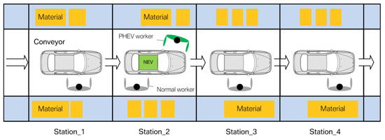
Figure 2.
Mixed-model assembly line under the floating pattern.
The study of the mixed-model assembly production under the floating pattern is based on the following conditions:
- (1)
- The mixed-model assembly line is a paced line, and the conveyor maintains a stable speed. The designed cycle time on each workstation is identical;
- (2)
- Models manufactured on the mixed-model assembly line are of similar size and chassis structure;
- (3)
- The sequence-dependent set-up times are not considered due to the process similarities among different models;
- (4)
- The PHEV is designed based on its same vehicle family gasoline vehicle; besides the powertrain system, two models have a lot of shared parts and common processes;
- (5)
- The common tasks among different models are assigned to the same workplace;
- (6)
- Duration variants of tasks among different models are allowed according to the practical processes.
When the floating pattern is adopted to deal with the production of PHEVs, PHEV workers are assigned to cover the extra components on PHEVs. Since the PHEV contains most components of the gasoline vehicle, the line balancing solution for the normal operators just needs little adjustment. Take the aforementioned BMW X1 (model code F49) and BMW X1 PHEV (model code F49 PHEV) as an example. These two cars share one mechanical chassis with the same structure. Design of the automotive exterior and interior is same on both types of vehicles. The cars’ cockpits maintain the similar style which is related to the order configuration. The major differences between the F49 and F49 PHEV are related to the modules of electric powertrain system which includes a high voltage battery unit, power electronic control unit, electric motor, charging unit, electric heater and related cables. Installations of these components are distributed to different sections in the assembly line. The real-world line balancing work is done according to specific line areas. Thus, the common operations shared by the F49 and F49 PHEV are performed by normal workers and the PHEV-specific parts are installed by the PHEV workers.
Thus, the mixed-model assembly line balancing can be done based on a combined precedence diagram [1]. Tasks of normal vehicles and the PHEVs are integrated into that precedence diagram. The precedence relationships in the combined diagram can be applied to different models produced on the assembly line.
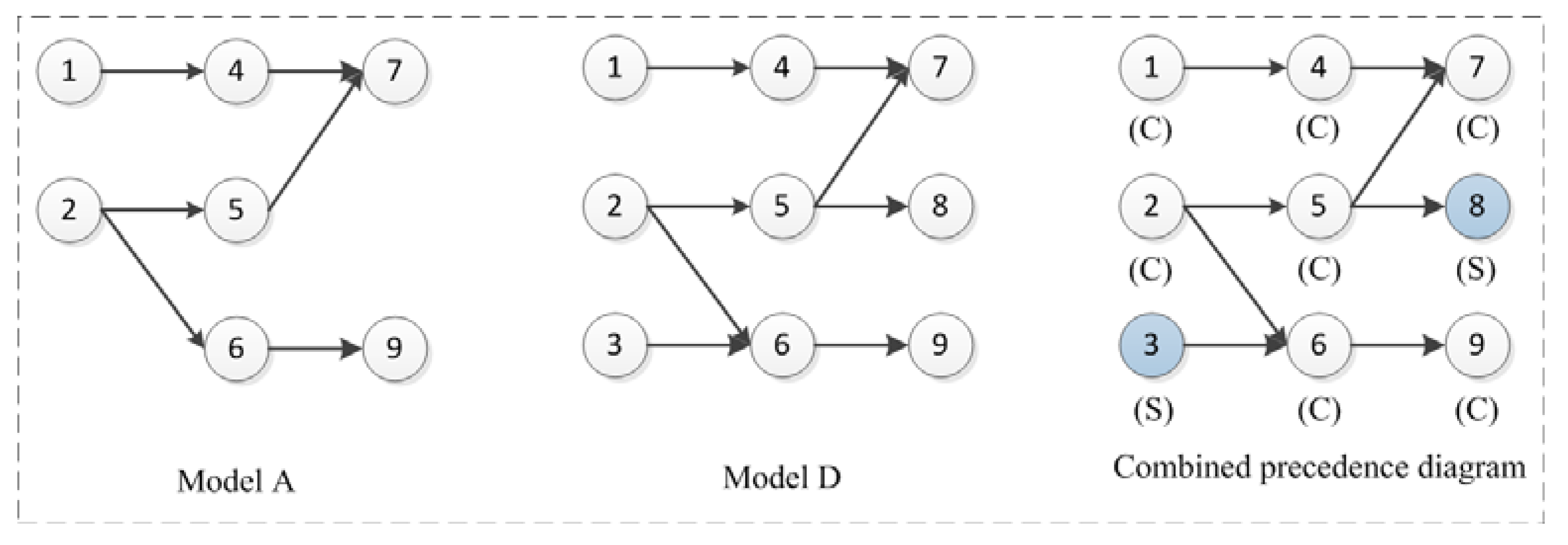
The task can be classified into two sets: the Common (C) task set and the Special (S) task set. The former contains the tasks that shared by both the PHEV model and the gasoline car. The later one is composed of the tasks which only belong to the PHEV model. Take the problem P9 with nine tasks as an example which is shown in Figure 3. The precedence relationship of P9 is taken from Ozcan and Toklu [41]. This example consists of two models: Model A and D. Model A is the normal gasoline car while Model D is the PHEV model. Task 1, 2, 4, 5, 6, 7 and 9 are the common tasks shared by both models; tasks 3 and 8 are the PHEV-specific operations. In the combined precedence diagram, these two types of tasks are denoted as C and S, respectively. The combined precedence diagram contains the tasks’ assembly relationships which can be applied to all models. Thus, the MALBP_F can be solved based on the combined precedence diagram. The method of computing the operation times of tasks in the combined precedence diagram will be introduced in Section 5.
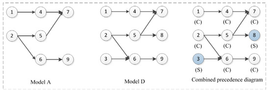
Figure 3.
Precedence diagrams of Model A, Model D and the combined diagram in problem P9.
Based on the methodologies stated above, the balancing problem of mixed-model assembly line with floating operators is similar to the Two-sided Assembly Line Balancing Problem (TALBP) where tasks have a positional characteristic [42]. A comprehensive review of the methods for solving the TALBP is presented by Li et al. [43]. In the TALBP, each workstation has two-faced positions (the left and the right position); task can be assigned to the left or the right according to its side preference. Although workers under the floating pattern are movable, not fixed to the workstation, the objective of the mixed-model line balancing problem can be set to minimize the total number of workstations. The mathematical model of MALBP_F is built in the following part.
3.2. Mathematical Model of MALBP_F
To simplify our presentation, the notations appeared in models are given at the end of this article.
The MALBP_F is solved based on the combined precedence diagram. Due to the strategy of utilizing the floating operators to take the additional jobs related to the PHEV, the number of workstations used for specific PHEV tasks process and common tasks processes are counted as the sum of Fj and Rj, respectively.
The objective function is to calculate the total number of workstations for the combined precedence diagram:
The mathematical model of MALBP_F is built as follows:
Subject to:
The decision variable xijk is set to represent on which workstation (j,k) task i is distributed, and it is the 0–1 binary variable (13). The workstation j is supposed to assemble the common task and the special task, and these two kinds of tasks are assigned to position r and position f, respectively.
Constraint (3) ensures that each task is distributed once to the workstation (j,k). The assembly process precedence is ensured by constraints (4)–(7). Tasks should be assigned to workstations no earlier than their predecessors (4). For tasks which have precedence relationships, constraint (5) is set to ensure that the assembly time of these tasks will not clash. One task can only start when all its predecessors have been finished if they ocurr at the same workstation j. One operator is not allowed to simultaneously conduct two assembly tasks, thus constraints (6) and (7) are active for tasks which have no precedence relationship. zip is the indicator variable which determines the assembly sequence of task i and p. When zip = 0, task p is planned before task i, the constraint set (6) is effective; when task i is arranged before task p, zip = 1, and the constraint set (7) becomes active. All tasks should be finished within the range of one cycle time as it is a paced assembly line (8). ||Wjk || represents the number of works assigned on workstation (j,k) (9) and (10). A workstation is counted as open if there is any task assigned on it, and binary variables Fj and Rj are set for counting the special PHEV workstations and normal workstations, respectively (11) and (12). Once there is one task i assigned to the k side of workstation j, the value of variable xijk is 1; accordingly, the value of Fj or Rj is equal to 1 (9)–(12).
Although our proposed model is built according the TALBP, some specific modifications are made to solve the MALBP_F. For example, in the model of Ozcan and Toklu [41], the primary objective is minimizing the number of mated-stations and the secondary objective is minimizing the number of operators. Considering the characteristic of the floating pattern of PHEV workers employed for NEV’s assembly production, the objective of MALBP_F minimizes the number of stations in our study. The VSP computes the minimum number of PHEV worker and jolly worker based on the line balancing results. Types of constraints are similar to the model of TALBP proposed by Ozcan and Toklu [41]. Our proposed model of MALBP simplifies the model by solving the problem based on the combined precedence diagram, while Ozcan and Toklu’s model deals with multi-models.
4. A Hierarchical Method to Solve the Line Balancing and Sequencing Problem
4.1. Hierarchical Procedure for Solving MALBP_F and VSP
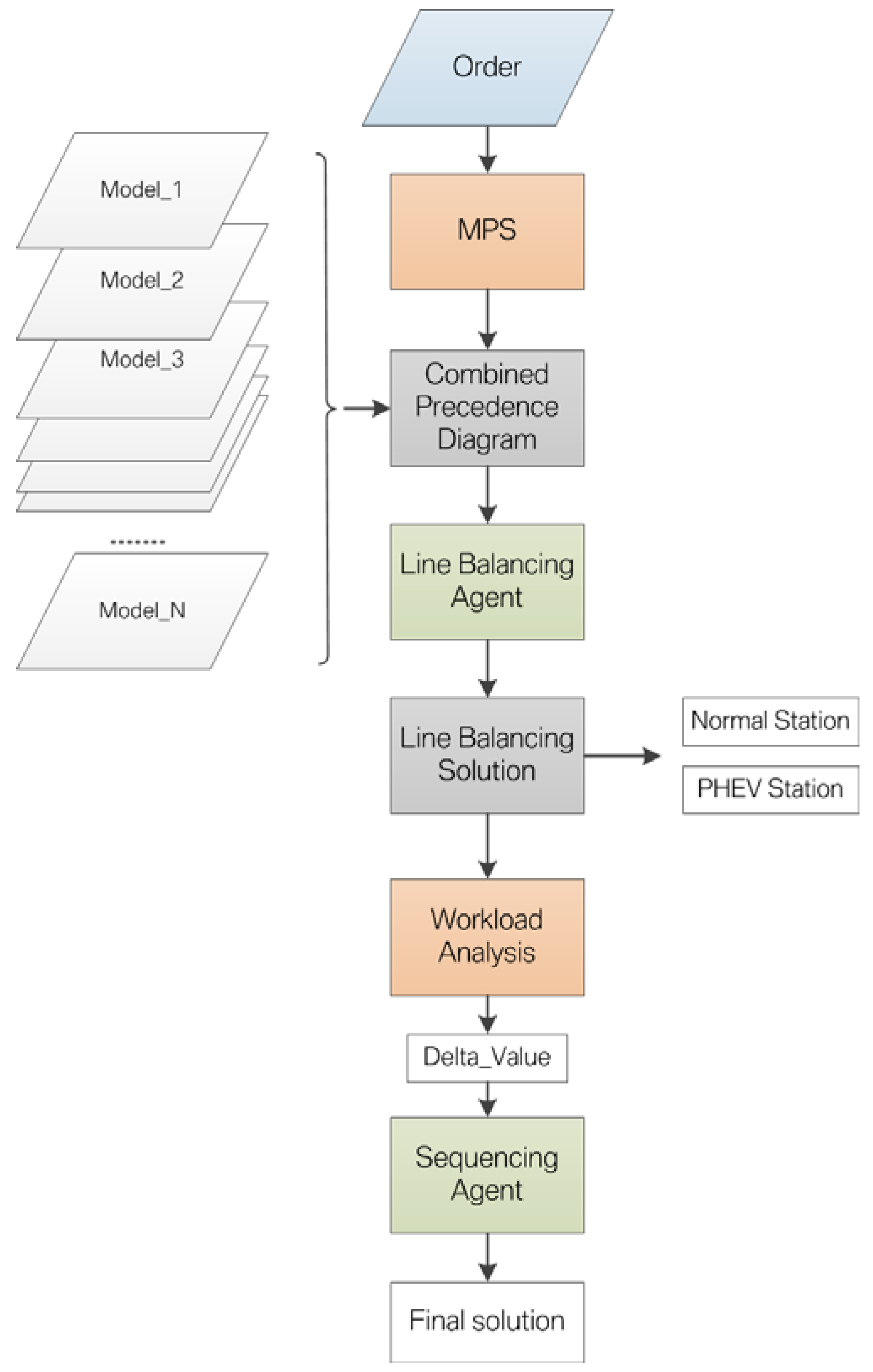
MALBP_F can be solved based on the combined precedence diagram. Results of line balancing can provide a reference for the assignment of tasks for all models. However, the real workload might be different due to the time variances among models. Overutilization occurs on some ‘heavy’ models when their total task time exceeds the cycle time; while underutilization of the cycle time happens if the vehicle has idle time after installations. Since the production system is a paced assembly line, any disturbance of the stable speed is undesirable. Thus, sequencing the vehicle models on the line is a necessary approach to maintain a balanced status of the mixed-model assembly system. We develop a hierarchical algorithm structure for solving the MALBP_F and VSP. Based the solutions of the MALBP_F and VSP, decision-makers at OEM can design the assembly process of vehicle’s components, arrange the workforce and schedule the manufacturing plan at the minimum production cost. The algorithm flow is shown in Figure 4. The Minimum Part Set (MPS) method is utilized in the sequencing problem. Through the repetitive production of the MPS, the volume of each model in the production plan can be satisfied [2]. The main contents of each step of the hierarchical algorithm is shown in Algorithm 1.
| Algorithm 1. Hierachical Procedure. | |
| 1: | Initialize a MPS list |
| 2: | Build the combined precedence diagram. |
| 3: | Solve the MALBP_F. |
| 4: | for each model in the MPS list do |
| 5: | calculate the delta value |
| 6: | end for |
| 7: | construct the model of VSP |
| 8: | solve the VSP |

Figure 4.
Algorithm flow of solving MALBP_F and VSP.
4.2. Vehicle Sequencing Problem for PHEV’s Production
Since the real processing time varies for different models, idle time and work-overload may occur. Normally, sequencing of launch models on the mixed-model assembly line deals with the overload caused by process variance. As assembly line is a paced production system which runs at a constant speed, so the time that the vehicle passes through each workstation is same. In every cycle time period, a new painted body is launched to the first station of the line and a completed vehicle is released from the final line. To measure the time in sequencing problem, the number of cycle times is set as p corresponding to the sequence number. The total number of workstations is counted as K, and the number of vehicle in the MPS list is D. Thus, the number of cycle time that all vehicles in the MPS pass K workstations is recorded as P in this study. The value of P is calculated as:
Take one MPS set [A, A, B, C, C] as an example. There are five cars of three models (A, B and C) in the MPS list, and they are produced in the sequence of ‘A-C-B-A-C’ as shown in Table 1. The assembly line has four workstations which denoted as Station_1, Station_2, Station_3 and Station_4. The time period starts when the first vehicle ‘A’ enters into Station_1 and ends when the last vehicle ‘C’ finishes all tasks at Station_4. Then, the next MPS is arriving at the line and will repeat the production cycles again. The sequence of vehicles in the MPS list can be applied to determine the production plan for one or several shifts.

Table 1.
An example of the production sequence of the MPS set.
According to the line balancing result, the processing time of the regular tasks of model m at station j is:
The difference between the processing time (model m at station j) and the cycle time is:
If the above total operating time exceeds the cycle time, there is an overloaded work situation at the station for the model m; if the operating time is less than or equal to the cycle time, there is no overloaded work. We calculate the work-overload of model m at station j as:
The ‘jolly worker’ is responsible for the part of general tasks that exceed the cycle time. The role of the jolly worker in the assembly line is very flexible in as much as they do not have a fixed working area. If there is a production line workstation where the normal staff cannot complete the assigned tasks within the cycle time, the jolly worker would move to that place and support them as a supplementary workforce. By configuring the jolly worker, the entire production line will not be stopped due to the overburdened status at one or several workstations. The labor force on the mixed-model assembly line under the floating pattern is composed of three types of staff: the ordinary operator, the PHEV worker, and the jolly worker. As explained earlier, the assembly tasks assigned to these three types of operators are different. In the solution of MALBP_F, the minimum number of ordinary operators required to complete the combined precedence diagram has been obtained. In this hierarchical algorithm, the objective function of VSP is to find the minimum number of PHEV workers and jolly workers. Denote the number of PHEV workers as N and the number of jolly workers as Ω, and the sum of these two values as H2:
The mathematical model of VSP is:
Subject to:
The decision variables of model sequence are set as Yw,m which are 0–1 integer variables. If model m is planned at w position in the sequence Yw,m = 1, and otherwise Yw,m = 0.
When calculating the number of PHEV workers and jolly workers, it is necessary to consider the situation when the greatest demand occurs. Therefore, the time span starts from the Kth cycle to the end of the (D + K − 1) cycle period. Within this range, it can be ensured that each station has one vehicle undergoing its assembly operations, and this time span fully takes into account the sequence combinations of vehicle models that may appear in the production area. From K to D cycle, the number of jolly workers required for overloaded stations must satisfy the constraint (21). From D + 1 to D + K − 1 cycle, the number of jolly workers required for overloaded stations must meet the constraint (22). Constraints (23) ensure that PHEV operators on the production line can finish all the specific parts’ installations for any given vehicle sequence from K to D cycle. Constraints (24) guarantee that all the specific PHEV tasks can be covered by the PHEV workers from D + 1 to D + K − 1 cycle. In the sequencing model, it must make sure that the number of each vehicle model in the sequencing result can match that value in the MPS set (25). Constraint (26) ensures the rationality and feasibility of sequence solution that only one vehicle model is assigned to each position.
5. Case Study
Numerical experiments of three problems, which are P9, P16 and P48, are carried out in this work. The basic data of these three problems are taken from the published works of Ozcan and Toklu [41] and Defersha and Mohebalizadehgashti [2]. The testing experiments of the proposed hierarchical algorithm are coded in Python 3. Both the models of MALBP_F and VSP are solved through Gurobi 9.1.2 which is called by the main function in the Python environment. The computer on which experiments are conducted has an Intel CoreTM i7-3770 3.40 GHz CPU and 8 GB RAM memory.
5.1. Test of Problem P9
The precedence diagrams for problem P9 are presented in Figure 3 and the operation times are listed in Table 2. Model A is taken directly from the example problem of Ozcan and Toklu [41]. Model D, which is developed based on Model A, is the PHEV model. Thus, the operation times of task 1 and 4 of Model D are set as 2 and 3, respectively. Task 3 and 8 are the PHEV-specific work, and their operation times are 1 and 3 according to the data of Model B in Ozcan and Toklu [41]. A task with 0 duration means that it is not included by the specific model. For the tasks related to the PHEVs’ specific parts, their task times are taken as 0 on the gasoline models. The duration of the common task (C) in the combined diagram is taken as the weighted average time. This value is calculated according to the task’s duration and the proportion of each model. Since PHEV workers are assigned to take these special tasks, the duration of the PHEV tasks (S) in the combined diagram is taken as same as that on the PHEV model. This method is applied to all instances of experiments in this study.

Table 2.
Operation time of each task of different models in problem P9.
The proportion of the gasoline model A to the PHEV model D varies from 9:1 to 4:6. Thus, the MPS is taken as [A, A, A, A, A, A, A, A, A, D], [A, A, A, A, A, A, A, A, D, D], [A, A, A, A, A, A, A, D, D, D], [A, A, A, A, A, A, D, D, D, D] and [A, A, A, A, D, D, D, D, D, D], respectively. To test the algorithm for different production line speeds, the Cycle Time (CT) is set as 4, 5, 6, 7 and 8, respectively. The line balancing and sequencing results for different scenarios are listed in Table 3. As the CT increases, the number of normal workers decreases from 4 to 2. The proportion of the PHEV model affects the number of normal workers a little. More PHEV workers are needed as the proportion of the PHEV model rises. Since the common tasks of Model A and Model D are the same, no deviations of these common tasks exist between each model’s duration and the weighted average duration. As a result, the number of jolly workers in problem P9 is zero. The number of variables (N_V) and the number of constraints (N_C) in the model of MALBP and VSP are presented in the result list. These values can measure the scale of the optimization problems.

Table 3.
Results of line balancing and sequencing of problem P9.
To evaluate the solution quality, the relative MIP optimality gap values reported by the Gurobi solver are recorded in the result lists. All instances of MALBP_F and VSP in problem P9 are solved with the gap value of zero.
5.2. Test of Problem P16
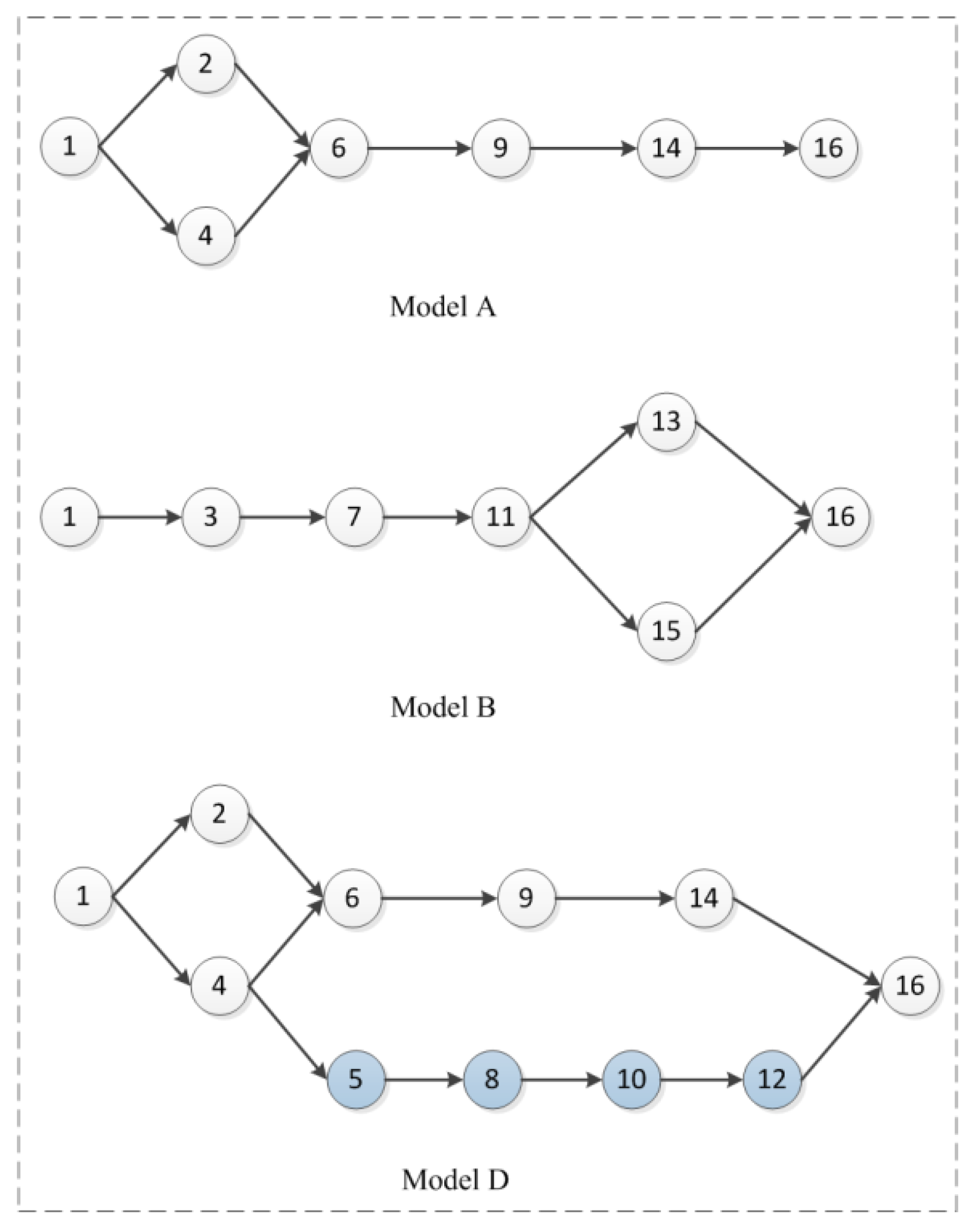
Problem P16, which has three models (Model A, B and D) and sixteen tasks in total, is designed based on the Problem-2 of Defersha and Mohebalizadehgashti [2]. The precedence diagrams of Model A, B, D and their combined precedence diagram are shown in Figure 5. Model A and B are normal gasoline cars, and Model D is the PHEV model. Model A maintains the same configuration as Model A of Problem-2 with the identical task duration and precedence diagram. Model B is modified by removing task 5, 8, 10, 12 and 14 of Problem-2′s Model B. Model D is the new designed PHEV model, and it is modified according to Problem-2′s Model C by adding task 4. Task 5, 8, 10, and 12 are specific PHEV tasks in P16. Operation time of each task in each model is presented in Table 4.
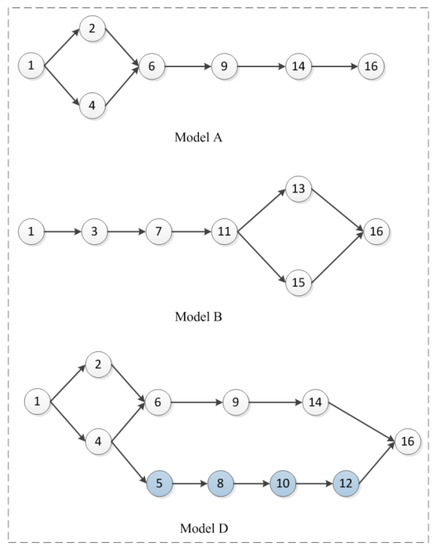
Figure 5.
Precedence diagram of each model in problem P16.

Table 4.
Operation time of each task of different models in problem P16.
Two model mixes are tested in problem P16: Models A, D and Models A, B, D. For the scenario of Models A, D, the proportion of the gasoline model A to the PHEV model D is set as 9:1, 8:2, 7:3, 6:4 and 4:6, respectively. The cycle time is set as 6, 8, 10, 12 and 14. Test results are listed in Table 5. With the ratio of Model D rising, the number of PHEV workers increases. Both the number of normal workers and PHEV workers decrease as the cycle time becomes longer. Also, no jolly workers are needed for production mix A, D of problem P16. Another production mix of problem P16 is Models A, B, D. The proportion of Model A to Model B to Model D is set as 4:5:1, 5:3:2, 3:4:3, 3:3:4 and 2:3:5 with the MPS of [A, A, A, A, B, B, B, B, B, D], [A, A, A, A, A, B, B, B, D, D], [A, A, A, B, B, B, B, D, D, D], [A, A, A, B, B, B, D, D, D, D] and [A, A, B, B, B, D, D, D, D, D], respectively. The number of normal workers decreases as the cycle time gets longer for all proportion scenarios. More PHEV workers are needed when the proportion of Model D increases. Jolly workers are necessary for production mix A, B, D due to the existence of Model B. The number of jolly workers varies as the proportion of Model B and the cycle time change. The gap values are also listed in Table 5. For instances of model mix A and D of MALBP_F, problems can be solved optimally. For instances of model mix A, B and D of MALBP_F, the gap value ranges from 0 to 0.33.

Table 5.
Results of line balancing and sequencing of problem P16.
5.3. Test of Problem P48
Problem P48 is constructed with reference to Problem-3 of Defersha and Mohebalizadehgashti [2]. Four models, which are Model A, B, C and D, are redesigned in problem P48. Model A, B and C are normal gasoline cars. Model D is defined as the PHEV model with specific PHEV task 6, 11, 16, 22, 28, 30, 34, 36, 40 and 44. The operation time of each task in each model is presented in Table 6. The precedence diagrams of four models are shown in Figure 6. Three production mix, which are Models A, D, Models A, B, D and Models A, B, C, D, are investigated in problem P48. The cycle time is set as 12, 14, 16, 18 and 20 for testing each proportion scenario. Since there are forty-eight tasks and four different models in problem P48, it is a large-sized mixed integer programming problem. The time limit of Gurobi solver is set as 300 s. A current best feasible solution is returned when this limit is reached.

Table 6.
Operation time of each task of different models in problem P48.
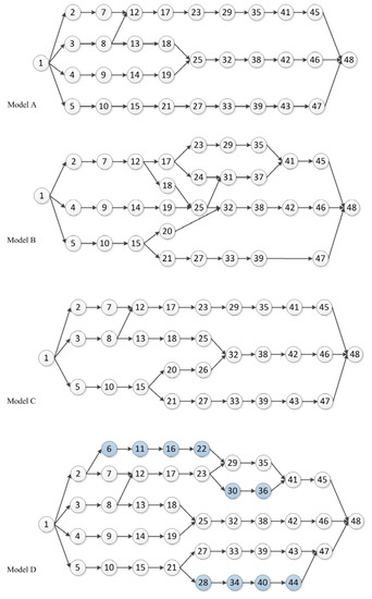
Figure 6.
Precedence diagram of each model in problem P48.
For model mix of Models A, D, the number of normal workers decreases as the CT increase. However, the number of normal workers under each cycle time remains the same for different proportions. The number of PHEV workers increases as the ratio of Model D rises. No jolly workers are needed for the products mix of Models A, D. For the model mix of Models A, B, D, five proportion scenarios (4:5:1, 3:5:2, 3:4:3, 3:3:4 and 2:3:5) are set in the experiment. The changes of the number of normal workers for different CTs are same in each proportion scenario. A clear trend is that the number of PHEV workers increases as the proportion of Model D rises. A jolly worker is needed in most cases of model mix of Model A, B, D. The third model mix of problem P48 is Models A, B, C, D. The proportions of four models are set as 3:3:3:1, 2:3:3:2, 2:3:2:3, 1:2:3:4 and 1:2:2:5, respectively. The numbers of normal workers are identical in different proportion scenarios for each CT. As the CT becomes longer, the number of normal workers decreases. The number of PHEV workers increases as the proportion of Model D rises in the products mix. One jolly worker is assigned in all scenarios of problem P48. Detailed results are shown in Table 7 and Table 8. As the number of tasks and model increase, the MALBP_F becomes harder to solve. The gap value of MALBP_F in problem P48 ranges from 0.75 to 0.86; while the VSP can still be solved with the gap value of zero.

Table 7.
First part of results of line balancing and sequencing of problem P48.

Table 8.
Second part of results of line balancing and sequencing of problem P48.
5.4. Test of Real-World Production Case
The integration of the BMW X1 PHEV (F49 PHEV) has been discussed in previous sections as a practical case of our research. Here we present an experiment study based on the real-world data related to the mixed-model assembly production of F49 PHEV at BMW-Brilliance Tiexi Plant. Three models with the same chassis structure were produced on one assembly line: model F49, model F49 PHEV and model F45. We select one section of the vehicle body components assembly on the main line. There were forty-one tasks in this case. The real cycle time of the production line was 88.2 s, and in each cycle the walking time used from one car to the next car was set as 6.2 s. Thus, the computing cycle time is obtained by the difference of the two values. The duration of each task of each model is recorded in Table 9. Twenty-one common tasks are taken on both F49 and F49 PHEV cars. The PHEV-specific tasks of model F49 PHEV are described in Table 10.

Table 9.
Operation time of each task of different models in problem BMW P41.

Table 10.
Description of specific tasks of F49 PHEV in problem BMW P41.
The initial production plan of the vehicles is producing one PHEV car every ten vehicles. In this test, the ratio of PHEV cars to normal cars is taken according to the values listed in Table 11. To unify the style of the sequence result, the F49, F45 and F49 PHEV are recorded as model A, model B, and model D, respectively. To test the proposed method for different products mix, the proportion of F49:F45:F49 PHEV is set as 5:4:1, 5:3:2, 3:4:3, 3:3:4 and 2:3:5, respectively. These ratios are created considering a possible increment of NEV demand in the future. Additionally, the cycle time is taken as 66, 70, 74, 78 and 82 for different production line speeds. The line balancing results and the vehicle sequence of problem P41 are presented in Table 11. Four normal workers are necessary for most instances, except for the case of ratio-5:3:2, CT-82. The number of PHEV workers increases from one to two when the proportion of F49 PHEV is larger than 20%. As the CT becomes shorter, more PHEV workers are needed to take on the tasks listed in above table. The number of variables (N_V) and the number of constraints (N_C) in the model of MALBP and VSP are counted in Table 11. The gap value of the MALBP_F of problem P41 ranges from 0.5 to 0.75. All instances of VSP are solved optimally in problem P41.

Table 11.
Results of line balancing and sequencing of the BMW P41 problem.
6. Conclusions
In this article, the floating pattern of an assembly production line with specific PHEV workers is studied. A hierarchical structure algorithm is presented to solve the MALBP_F and VSP for the first time. Mathematical formulations are built for the MALBP_F and VSP, respectively. A mixed integer programming model is presented for the MALBP_F. An integer programming model is developed to solve the VSP under the floating pattern based on the line balancing results. The proposed hierarchical algorithm can solve the MALBP_F and VSP exactly aiming to achieve the minimum number of workstations and total workers. The difficulty in solving procedure is that the scale of MALBP_F is much larger than that of VSP. More variables and constraints are contained in the model of MALBP_F which makes it hard to obtain the optimal solution in short time.
Numerical experiments are conducted to verify the effectiveness and the efficiency of the proposed method. Three novel problems that include the new energy vehicle model (PHEV) are designed. One problem with the real-world automotive production data is presented. To illustrate the algorithm’s performance, this study tests instances of different model mix and various proportion scenarios. The obtained results show that the developed algorithm can get optimal solutions on most instances of the small and middle scale problems (P9, P16). The relative optimality gap of MALBP_F returned from the Gurobi solver range from 0 to 0.33. For the large-scale problems (P41, P48), the algorithm can still return the incumbent solutions with the gap values range from 0.5 to 0.86. The VSP is easier to solve with much fewer variables and constraints. All instances of VSP are optimally solved with the gap value of zero. A changing trend of the results of all instances show that the number of normal workers varies little as the proportion fluctuates. However, the number of PHEV workers increases when the ratio of PHEV models rises. This demonstrates the advantage of the floating production pattern’s flexibility. The fluctuations of the NEV orders can be mitigated mainly by adjusting the number of PHEV workers. Thus, the influence on the production system caused by the integration of NEVs will be minimized. The current approach has limitations in finding optimal solutions for large-scale problems because of their NP-hard characteristic. Thus, more powerful algorithms for the MALBP_F are needed to solve these problems efficiently and optimally. Furthermore, studies considering more practical constraints, such as zoning constraints, unique line configurations and stochastic factors, that happen in real assembly production lines may be of interest in future work.
Author Contributions
Conceptualization, J.H. and Q.Y.; methodology, Q.Y.; software, Q.Y.; validation, Q.Y., X.L. and J.H.; formal analysis, X.L.; investigation, J.H.; resources, J.H.; writing—original draft preparation, Q.Y.; writing—review and editing, X.L.; visualization, Q.Y.; supervision, X.L.; funding acquisition, X.L. All authors have read and agreed to the published version of the manuscript.
Funding
This research was supported by National Key R&D Program of China (Grant No.: 2019YFB1705002, Grant No.: 2017YFB0304100), National Natural Science Foundation of China (Grant No.: 51634002), LiaoNing Revitalization Talents Program (Grant No.: XLYC2002041).
Institutional Review Board Statement
Not applicable.
Informed Consent Statement
Not applicable.
Data Availability Statement
Data supporting reported results can be found in this manuscript.
Acknowledgments
This research topic was raised and supported at the BMW-Brilliance Automotive Company. Authors were members of ProMotion Ph.D. project initiated by BMW-Brilliance Automotive Company and Northeastern University.
Conflicts of Interest
The authors declare no conflict of interest.
Abbreviations
| Indices | |
| i,h,p | task number |
| j,g | mated-station |
| k | side of the assembly line |
| Parameters | |
| I | set of tasks |
| IC | set of common tasks |
| IS | set of specific PHEV tasks |
| J | set of workstations |
| K(i) | set of available positions of the task i |
| P0 | set of task which has no immediate predecessor |
| P(i) | set of immediate predecessors of task i |
| Pa(i) | set of total tasks which precede task i |
| Sa(i) | set of total tasks which follow task i |
| ct | cycle time |
| ti | operation time of task i |
| μ | multiplier as the big M |
| dm | value demand of model m |
| Variables | |
| xijk | if task i is assigned to side k of station j, =1; otherwise, =0 |
| H1 | number of total workstations |
| H2 | number of supplementary workers |
| Fj | if station j is open for PHEV tasks’ assembly, =1; otherwise, =0 |
| Rj | if station j is open for common tasks’ assembly, =1; otherwise, =0 |
| finish time of task i | |
| zip | indicator variable to represent assembly sequence of task i and p |
| Wjk | set of tasks assigned to station(j,k) |
| Yw,m | if model m is arranged at position w, =1; otherwise, =0 |
| N | number of jolly workers |
| Ω | number of PHEV workers |
References
- Ramezanian, R.; Ezzatpanah, A. Modeling and solving multi-objective mixed-model assembly line balancing and worker assignment problem. Comput. Ind. Eng. 2015, 87, 74–80. [Google Scholar] [CrossRef]
- Defersha, F.M.; Mohebalizadehgashti, F. Simultaneous balancing, sequencing, and workstation planning for a mixed model manual assembly line using hybrid genetic algorithm. Comput. Ind. Eng. 2018, 87, 74–80. [Google Scholar] [CrossRef]
- Battaia, O.; Dolgui, A. A taxonomy of line balancing problems and their solution approaches. Int. J. Prod. Econ. 2013, 142, 259–277. [Google Scholar] [CrossRef]
- Eghtesadifard, M.; Khalifeh, M.; Khorram, M. A systematic review of research themes and hot topics in assembly line balancing through the web of science within 1990–2017. Comput. Ind. Eng. 2020, 139, 106182. [Google Scholar] [CrossRef]
- Boysen, N.; Fliedner, M.; Scholl, A. Sequencing mixed-model assembly lines: Survey, classification and model critique. Eur. J. Oper. Res. 2009, 192, 349–373. [Google Scholar] [CrossRef]
- Simaria, A.S.; Vilarinho, P.M. A genetic algorithm based approach to the mixed-model assembly line balancing problem of type ii. Comput. Ind. Eng. 2004, 47, 391–407. [Google Scholar] [CrossRef]
- Bukchin, Y.; Rabinowitch, I. A branch-and-bound based solution approach for the mixed-model assembly line-balancing problem for minimizing stations and task duplication costs. Eur. J. Oper. Res. 2006, 174, 492–508. [Google Scholar] [CrossRef]
- Yagmahan, B. Mixed-model assembly line balancing using a multi-objective ant colony optimization approach. Expert Syst. Appl. 2011, 38, 12453–12461. [Google Scholar] [CrossRef]
- Manavizadeh, N.; Rabbani, M.; Moshtaghi, D.; Jolai, F. Mixed-model assembly line balancing in the make-to-order and stochastic environment using multi-objective evolutionary algorithms. Expert Syst. Appl. 2012, 39, 12026–12031. [Google Scholar] [CrossRef]
- Hyun, C.J.; Kim, Y.; Kim, Y.K. A genetic algorithm for multiple objective sequencing problems in mixed model assembly lines. Comput. Oper. Res. 1998, 25, 675–690. [Google Scholar] [CrossRef]
- McMullen, P.R.; Frazier, G.V. A simulated annealing approach to mixed-model sequencing with multiple objectives on a just-in-time line. IIE Trans. 2000, 32, 679–686. [Google Scholar] [CrossRef]
- Ishigaki, A.; Miyashita, T. Development of search method for sequencing problem in mixed-model assembly lines. J. Adv. Mech. Des. Syst. Manuf. 2016, 10, JAMDSM0048. [Google Scholar] [CrossRef]
- Bautista, J.; Alfaro-Pozo, R.; Batalla-García, C. Grasp for sequencing mixed models in an assembly line with work overload, useless time and production regularity. Prog. Artif. Intell. 2016, 5, 27–33. [Google Scholar] [CrossRef][Green Version]
- Bautista, J.; Cano, A.; Alfaro-Pozo, R. A hybrid dynamic programming for solving a mixed-model sequencing problem with production mix restriction and free interruptions. Prog. Artif. Intell. 2017, 6, 27–39. [Google Scholar] [CrossRef]
- Hwang, R.; Katayama, H. Integrated procedure of balancing and sequencing for mixed-model assembly lines: A multi-objective evolutionary approach. Int. J. Prod. Res. 2010, 48, 6417–6441. [Google Scholar] [CrossRef]
- Faccio, M.; Gamberi, M.; Bortolini, M. Hierarchical approach for paced mixed-model assembly line balancing and sequencing with jolly operators. Int. J. Prod. Res. 2016, 54, 761–777. [Google Scholar] [CrossRef]
- Kim, Y.K.; Kim, J.Y.; Kim, Y. A coevolutionary algorithm for balancing and sequencing in mixed model assembly lines. Appl. Intell. 2000, 13, 247–258. [Google Scholar] [CrossRef]
- Mosadegh, H.; Ghomi, S.F.; Zandieh, M. Simultaneous solving of balancing and sequencing problems in mixed-model assembly line systems. Int. J. Prod. Res. 2012, 50, 4994–5016. [Google Scholar] [CrossRef]
- Saif, U.; Guan, Z.; Liu, W.; Wang, B.; Zhang, C. Multi-objective artificial bee colony algorithm for simultaneous sequencing and balancing of mixed model assembly line. Int. J. Adv. Manuf. Technol. 2014, 75, 1809–1827. [Google Scholar] [CrossRef]
- Manavizadeh, N.; Rabbani, M.; Radmehr, F. A new multi-objective approach in order to balancing and sequencing u-shaped mixed model assembly line problem: A proposed heuristic algorithm. Int. J. Adv. Manuf. Technol. 2015, 79, 415–425. [Google Scholar] [CrossRef]
- Kucukkoc, I.; Zhang, D.Z. Integrating ant colony and genetic algorithms in the balancing and scheduling of complex assembly lines. Int. J. Adv. Manuf. Technol. 2016, 82, 265–285. [Google Scholar] [CrossRef]
- Kim, Y.K.; Kim, S.J.; Kim, J.Y. Balancing and sequencing mixed-model U-lines with a co-evolutionary algorithm. Prod. Plan. Control. 2000, 11, 754–764. [Google Scholar] [CrossRef]
- Kim, Y.K.; Kim, J.Y.; Kim, Y. An endosymbiotic evolutionary algorithm for the integration of balancing and sequencing in mixed-model U-lines. Eur. J. Oper. Res. 2006, 168, 838–852. [Google Scholar] [CrossRef]
- Rabbani, M.; Kazemi, S.M.; Manavizadeh, N. Mixed model U-line balancing type-1 problem: A new approach. J. Manuf. Syst. 2012, 31, 131–138. [Google Scholar] [CrossRef]
- Rabbani, M.; Montazeri, M.; Farrokhi-Asl, H.; Rafiei, H. A multi-objective genetic algorithm for a mixed-model assembly u-line balancing type-i problem considering human-related issues, training, and learning. J. Ind. Eng. Int. 2016, 12, 485–497. [Google Scholar] [CrossRef][Green Version]
- Mosadegh, H.; Zandieh, M.; Ghomi, S.F. Simultaneous solving of balancing and sequencing problems with station-dependent assembly times for mixed-model assembly lines. Appl. Soft. Comput. 2012, 12, 1359–1370. [Google Scholar] [CrossRef]
- Vilarinho, P.M.; Simaria, A.S. Antbal: An ant colony optimization algorithm for balancing mixed-model assembly lines with parallel workstations. International Journal of Production Research. Int. J. Prod. Res. 2006, 44, 291–303. [Google Scholar] [CrossRef]
- Rabbani, M.; Siadatian, R.; Farrokhi-Asl, H.; Manavizadeh, N. Multi-objective optimization algorithms for mixed model assembly line balancing problem with parallel workstations. Cog. Eng. 2016, 3, 1158903. [Google Scholar] [CrossRef]
- Kucukkoc, I.; Zhang, D.Z. Mixed-model parallel two-sided assembly line balancing problem: A flexible agent-based ant colony optimization approach. Comput. Ind. Eng. 2016, 97, 58–72. [Google Scholar] [CrossRef]
- Akpinar, S.; Baykasoglu, A. Modeling and solving mixed-model assembly line balancing problem with setups. Part i: A mixed integer linear programming model. J. Manuf. Syst. 2014, 33, 177–187. [Google Scholar] [CrossRef]
- Akpinar, S.; Baykasoglu, A. Modeling and solving mixed-model assembly line balancing problem with setups. Part II: A multiple colony hybrid bees algorithm. J. Manuf. Syst. 2014, 33, 445–461. [Google Scholar] [CrossRef]
- Zhao, X.; Hsu, C.; Li, L.P. A genetic algorithm for the multi-objective optimization of mixed-model assembly line based on the mental workload. Eng. Appl. Artif. Intell. 2016, 47, 140–146. [Google Scholar] [CrossRef]
- Dimitriadis, S.G. Assembly line balancing and group working: A heuristic procedure for workers’ groups operating on the same product and workstation. Comput. Oper. Res. 2006, 33, 2757–2774. [Google Scholar] [CrossRef]
- Becker, C.; Scholl, A. Balancing assembly lines with variable parallel workplaces: Problem definition and effective solution procedure. Eur. J. Oper. Res. 2009, 199, 359–374. [Google Scholar] [CrossRef]
- Fattahi, P.; Roshani, A.; Roshani, A. A mathematical model and ant colony algorithm for multi-manned assembly line balancing problem. Int. J. Adv. Manuf. Technol. 2011, 53, 363–378. [Google Scholar] [CrossRef]
- Yazdanparast, V.; Hajihosseini, H. Multi-manned production lines with labor concentration. Aust. J. Basic Appl. Sci. 2011, 5, 839–846. [Google Scholar]
- Kazemi, A.; Sedighi, A. A cost-oriented model for balancing mixed-model assembly lines with multi-manned workstations. Int. J. Serv. Oper. Manag. 2013, 16, 289–309. [Google Scholar] [CrossRef]
- Roshani, A.; Nezami, F.G. Mixed-model multi-manned assembly line balancing problem: A mathematical model and a simulated annealing approach. Assem. Autom. 2017, 37, 34–50. [Google Scholar] [CrossRef]
- Kellegoz, T. Assembly line balancing problems with multi-manned stations: A new mathematical formulation and Gantt based heuristic method. Ann. Oper. Res. 2016, 253, 377–404. [Google Scholar] [CrossRef]
- Kellegoz, T.; Toklu, B. A priority rule-based constructive heuristic and an improvement method for balancing assembly lines with parallel multi-manned workstations. Int. J. Prod. Res. 2015, 53, 736–756. [Google Scholar] [CrossRef]
- Ozcan, U.; Toklu, B. Balancing of mixed-model two-sided assembly lines. Comput. Ind. Eng. 2009, 57, 217–227. [Google Scholar] [CrossRef]
- Li, Z.; Kucukkoc, I.; Zhang, Z. Branch, bound and remember algorithm for two-sided assembly line balancing problem. Eur. J. Oper. Res. 2020, 284, 896–905. [Google Scholar] [CrossRef]
- Li, Z.; Kucukkoc, I.; Nilakantan, J.M. Comprehensive review and evaluation of heuristics and meta-heuristics for two-sided assembly line balancing. Comput. Oper. Res. 2017, 84, 146–161. [Google Scholar] [CrossRef]
Publisher’s Note: MDPI stays neutral with regard to jurisdictional claims in published maps and institutional affiliations. |
© 2021 by the authors. Licensee MDPI, Basel, Switzerland. This article is an open access article distributed under the terms and conditions of the Creative Commons Attribution (CC BY) license (https://creativecommons.org/licenses/by/4.0/).

