
Prediction of Abrasive Belt Wear Based on BP Neural Network

Abstract
:1. Introduction
2. State of the Art
3. Wear Prediction Based on BP Neural Network
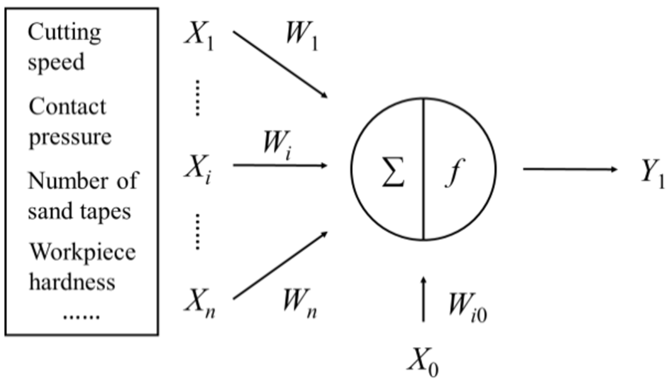
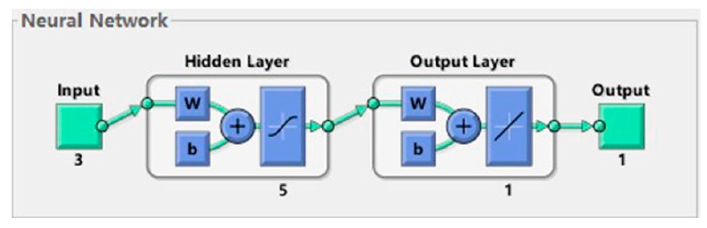
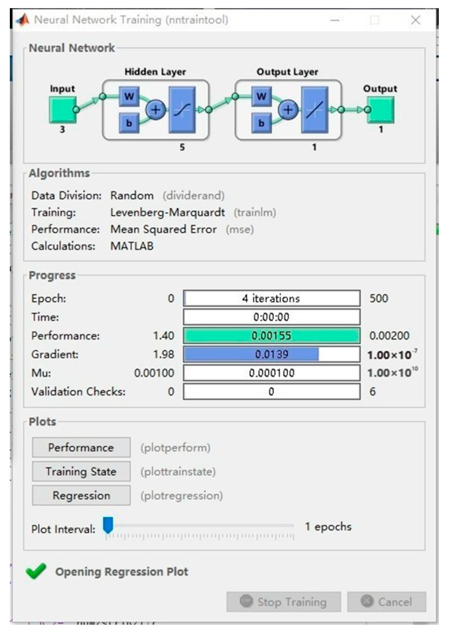
3.1. BP Neuron Structure
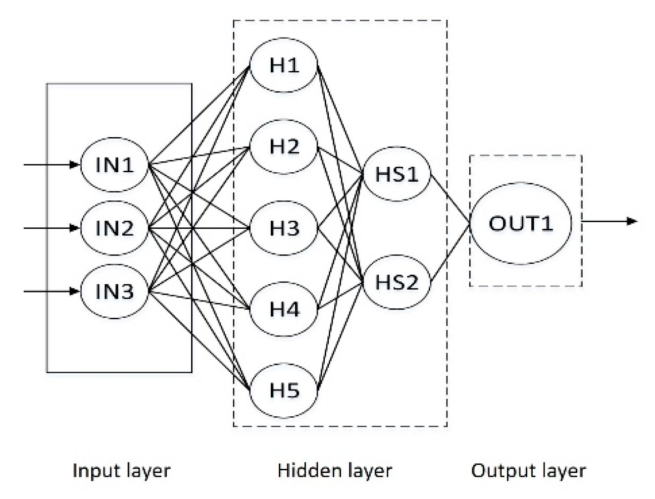
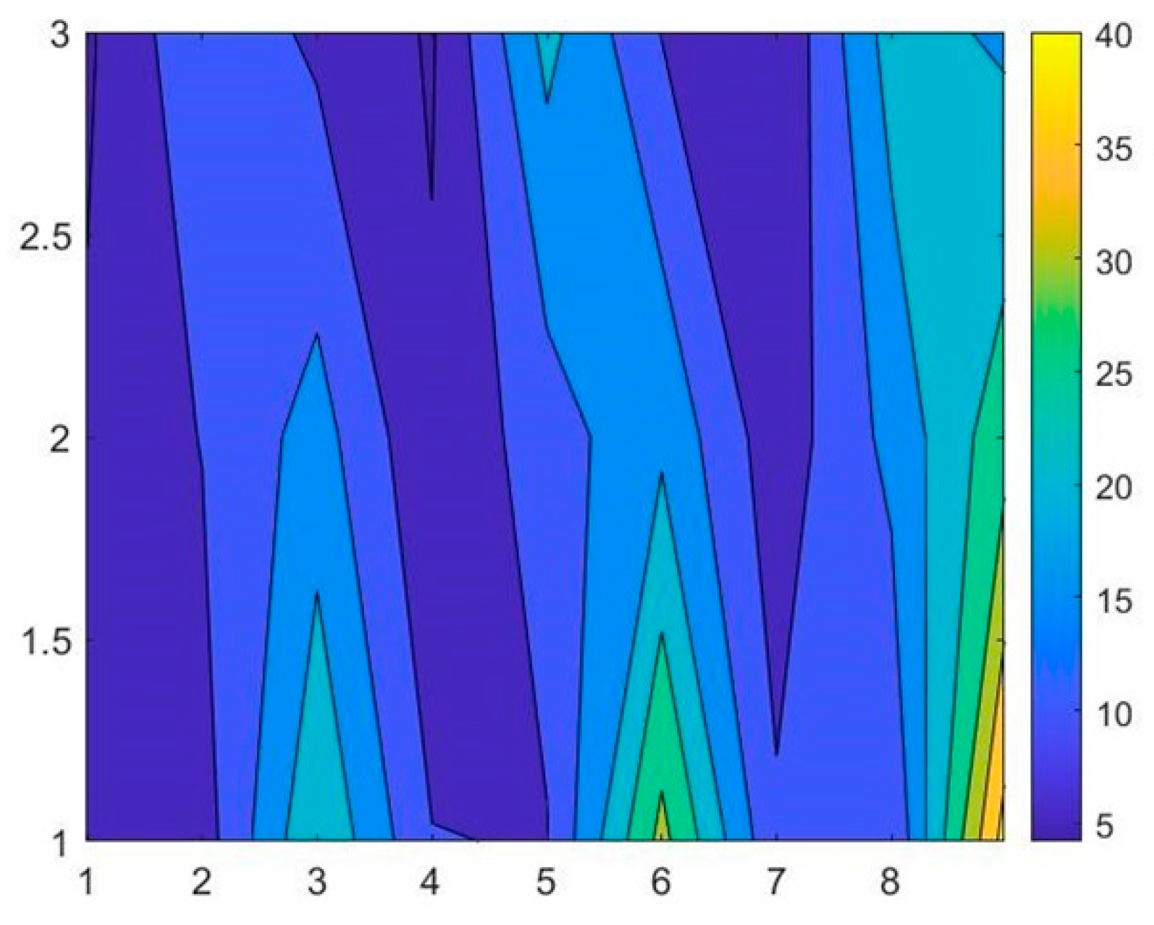
3.2. Setting of BP Neuron Topology Parameter
3.3. BP Process and Data Processing
4. Abrasive Belt Wear Measurement Test
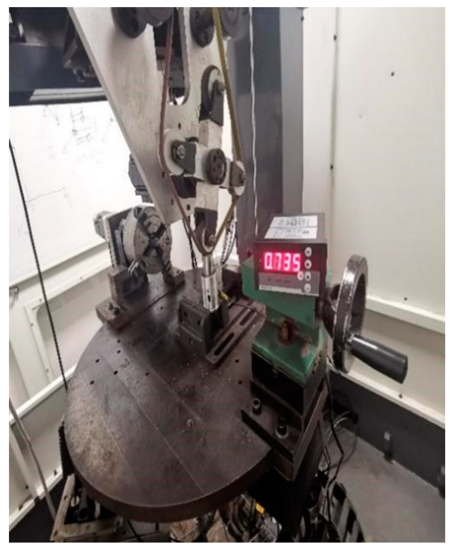
4.1. Test Equipment and Testing Equipment
4.2. Experimental Parameters
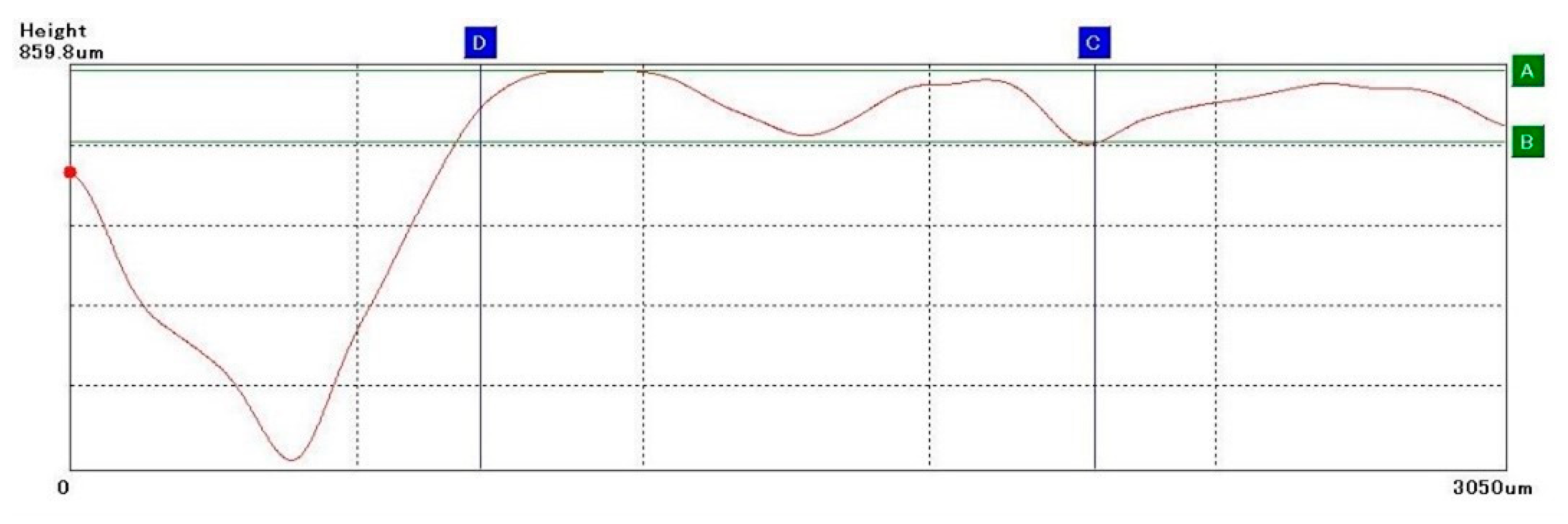
4.3. Detection Error Control
4.4. Test Results
4.5. Test Data Analysis
5. BP Neural Network Experimental Analysis
5.1. Data Analysis
5.2. Principles of Experimental Analysis
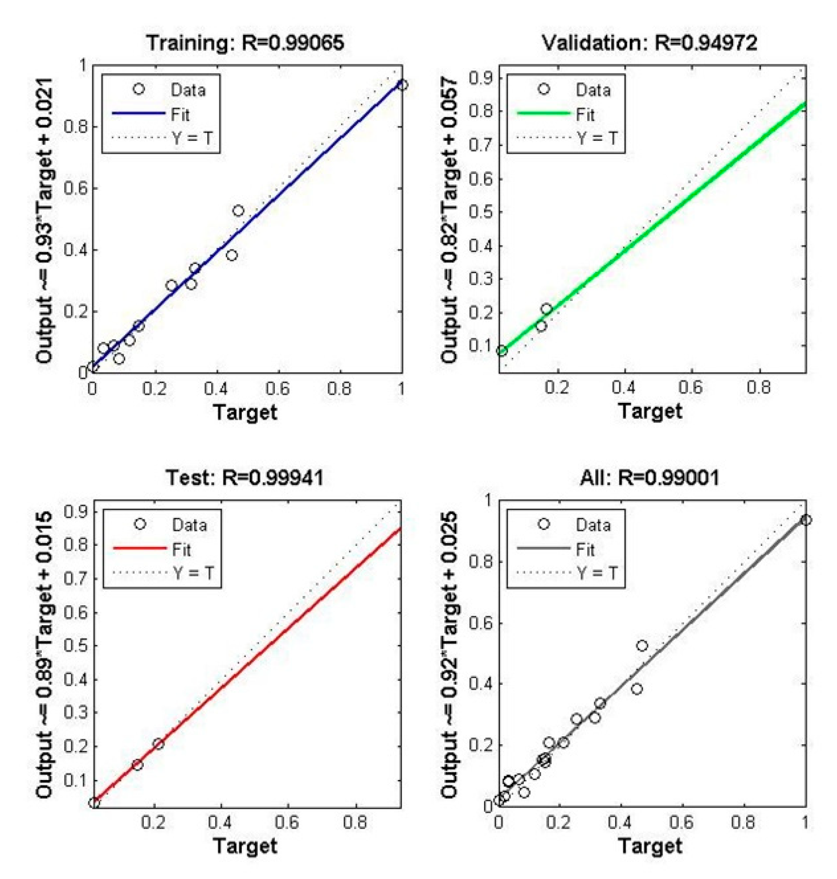
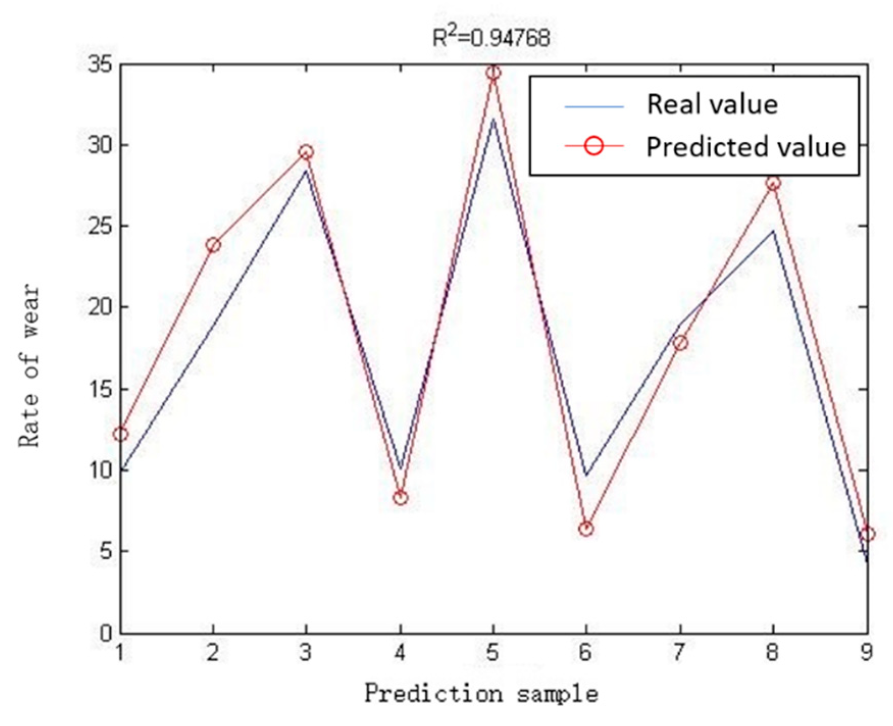
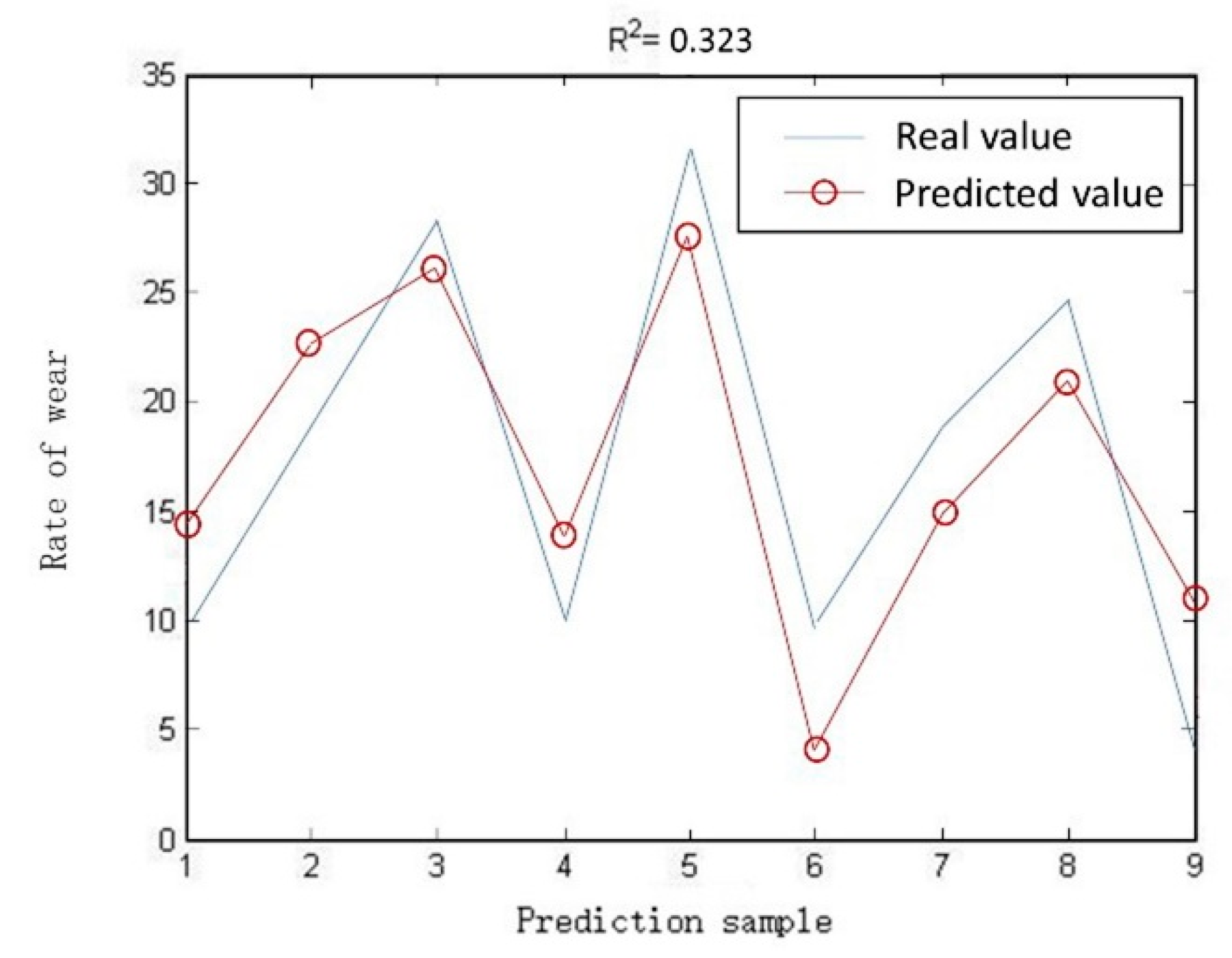
5.3. Comparison of Experimental Results
6. Conclusions
Author Contributions
Funding
Institutional Review Board Statement
Informed Consent Statement
Data Availability Statement
Conflicts of Interest
References
- Xiao, G.; Song, K.; Liu, S.; Wu, Y.; Wang, W. Comprehensive investigation into the effects of relative grinding direction on abrasive belt grinding process. J. Manuf. Process. 2021, 62, 753–761. [Google Scholar] [CrossRef]
- Zhang, P.; Li, J. Steel Wire Grinding Testing Based on New Type Abrasive Belt Grinding Machine. Adv. Mater. Res. 2013, 602–604, 2273–2278. [Google Scholar] [CrossRef]
- Rech, J.; Moisan, A. Belt grinding: A way to optimize the surface integrity of cut surfaces. In Proceedings of the 3rd International Conference on Machining and Measurements of Sculptured Surfaces (MMSS), Kraków, Poland, 20–22 September 2003; pp. 125–132. [Google Scholar]
- Denkena, B.; Grove, T.; Suntharakumaran, V. New profiling approach with geometrically defined cutting edges for sintered metal bonded CBN grinding layers. J. Mater. Process. Technol. 2019, 278, 116473. [Google Scholar] [CrossRef]
- Namba, Y.; Tsuwa, H. Evaluation of Abrasive Belt Performance. J. Jpn. Soc. Precis. Eng. 1976, 42, 828–833. [Google Scholar] [CrossRef]
- Lemaster, R.; Dornfeld, D. The use of acoustic emission to monitor an abrasive machining process. In Proceedings of the 11th International Wood Machining Seminar, Honne, Norway, 25–27 May 1993; pp. 231–245. [Google Scholar]
- Chen, J.; Wang, J.; Zhang, X.; Cao, F.; Chen, X. Acoustic signal-based tool wear monitoring system for belt grinding of superalloys. In Proceedings of the 2017 12th IEEE Conference on Industrial Electronics and Applications, Siem Reap, Cambodia, 18–20 June 2017; pp. 1281–1286. [Google Scholar]
- Ferguson, D.C.; Kolecki, J.C.; Siebert, M.W.; Wilt, D.M.; Matijevic, J.R. Evidence for Martian electrostatic charging and abrasive wheel wear from the wheel abrasion experiment on the Pathfinder Sojourner Rover. J. Geophys. Res. 1999, 104, 8747–8789. [Google Scholar] [CrossRef] [Green Version]
- Malinov, L.S.; Malysheva, I.E.; Klimov, E.S.; Kukhar, V.V.; Balalayeva, E.Y. Effect of particular combinations of quenching, tempering and carburization on abrasive wear of low-carbon manganese steels with metastable austenite. Mater. Sci. Forum 2019, 945, 574–578. [Google Scholar] [CrossRef]
- Carrano, A.L.; Vora, B.S.; Sahin, F.; Lemaster, R.L. Monitoring of abrasive loading for optimal belt cleaning or replacement. For. Prod. J. 2007, 57, 78–83. [Google Scholar]
- Fuhua, S. Prediction of grinding wheel life of shaving machine based on improved gray GM (1, N) model. China Leather 2016, 45, 16–19. [Google Scholar]
- Zhi, G.; Li, X.; Qian, Z.; Liu, H.; Rong, Y. Experimental study of time-dependent performance in superalloy high-speed grinding with cBN wheels. Mach. Sci. Technol. 2016, 20, 615–633. [Google Scholar] [CrossRef]
- Wanshan, W.; Ruilan, S. A Study on the Wear Mechanism of Abrasive Belt in Grinding Nickel Metal. Diamond Abrasives Eng. 1990, 4, 11–16. [Google Scholar]
- Leyin, X.; Feng, L.; Delong, X.; Xiaoyi, P. Study of the Influences of Different Factors on Diamond Soft Grinding Wheel Abrasion. Superhard Mater. Eng. 2016, 28, 1–5. [Google Scholar]
- McGibbon, T.R.; Amundson, S.E.; Lokken, R.C. CAMOS: A computer-aided system for establishing optimal parameters for achieving uniform abrasive wear during high-rate grinding. Wear 1976, 37, 1–200. [Google Scholar] [CrossRef]
- Maxence, B.; Benjamin, H. Mechanical modeling of micro-scale abrasion in superfinish belt grinding. Tribology 2008, 41, 992–1001. [Google Scholar]
- Mezghani, S.; Sura, M. Wear mechanism maps for the belt finishing of steel and cast iron. Wear 2009, 267, 86–91. [Google Scholar] [CrossRef]
- Peter, J.B.; Brian, C.J. Relationships between abrasive wear, hardness and grinding characteristics of Titanium-based Metal-Matrix composites. J. Mater. Eng. Perform. 2009, 18, 424–432. [Google Scholar]
- Cui, W.; Liu, J.; Li, H. Detecting grinding force of abrasive belt based on LabVIEW. Diam. Abras. Eng. 2014, 34, 80–83. [Google Scholar]
- Böhm, J.; Vernes, A.; Vorlaufer, G.; Vellekoop, M. Online monitoring of a belt grinding process by using a light scattering method. Appl. Opt. 2010, 49, 5891–5898. [Google Scholar] [CrossRef]
- Zawada, A.; Sciegienka, R. Monitoring of a micro-smoothing process with the use of machined surface images. Metrol. Meas. Syst. 2011, 18, 419–428. [Google Scholar]
- Song, S.; Xiong, X.; Wu, X.; Xue, Z. Modeling the SOFC by BP neural network algorithm. Int. J. Hydrogen Energy 2021, 46, 20065–20077. [Google Scholar] [CrossRef]
- Kechagias, J.D.; Tsiolikas, A.; Petousis, M.; Ninikas, K.; Vidakis, N.; Tzounis, L. A robust methodology for optimizing the topology and the learning parameters of an ANN for accurate predictions of laser-cut edges surface roughness. Simul. Model. Pract. Theory 2022, 114, 102414. [Google Scholar] [CrossRef]
- Basheer, I.A.; Haimeer, M. Artificial neural networks: Fundamentals, computing, design, and application. J. Microbiol. Methods 2000, 43, 3–31. [Google Scholar] [CrossRef]
- Kang, Y.; Choi, S. Restricted deep belief networks for multi-view learning. Mach. Learn. Knowl. Discov. Databases 2011, 130–145. [Google Scholar]
- Hajduk, Z. Hardware Implementation of Hyperbolic Tangent and Sigmoid Activation Function. Bull. Pol. Acad. Sci. Tech. Sci. 2018, 66, 563–577. [Google Scholar]
- Ardeshiri, R.R.; Ma, C. Multivariate gated recurrent unit for battery remaining useful life prediction: A deep learning approach. Int. J. Energy Res. 2021, 45, 16633–16648. [Google Scholar] [CrossRef]
- Li, A.; Chen, J. Summarize of Parameter Improve Methods for BP Neural Network. Digit. Commun. World 2009, 1, 62–64. [Google Scholar]
- Chen, L.; Guo, J.; Yang, X.; Xia, Z. Grinding roughness prediction model based on evolutionary artificial neural network. Comput. Integr. Manuf. Syst. 2013, 19, 2855–2859. [Google Scholar]
- Namba, Y.; Tsuwa, H. Machining Efficiency on Centerless Belt Grinding. J. Jpn. Soc. Precis. Eng. 1976, 42, 942–947. [Google Scholar] [CrossRef]
- Kitajima, K.; Tanaka, Y. Grinding Temperature and Affected Layer. J. Jpn. Soc. Precis. Eng. 1978, 44, 220–225. [Google Scholar] [CrossRef]
- Wang, W.X.; Li, J.Y.; Fan, W.G.; He, Z. Abrasion Process Modeling of Abrasive Belt Grinding in Rail Maintenance. J. Southwest Jiaotong Univ. 2017, 52, 141–147. [Google Scholar]
- Choudhury, S.K.; Srinivas, P. Tool wear prediction in turning. J. Mater. Process. Technol. 2004, 153, 276–280. [Google Scholar] [CrossRef]


| Trial Number | Cutting Speed (m/s) | Contact Force (N) | Experimental Material |
|---|---|---|---|
| 1 | 8 | 5 | #20 |
| 2 | 5 | 5 | #20 |
| 3 | 2 | 5 | #20 |
| 4 | 2 | 10 | #20 |
| 5 | 5 | 10 | #20 |
| 6 | 8 | 10 | #20 |
| 7 | 8 | 15 | #20 |
| 8 | 5 | 15 | #20 |
| 9 | 2 | 15 | #20 |
| 10 | 8 | 5 | #45 |
| 11 | 5 | 5 | #45 |
| 12 | 2 | 5 | #45 |
| 13 | 2 | 10 | #45 |
| 14 | 5 | 10 | #45 |
| 15 | 8 | 10 | #45 |
| 16 | 8 | 15 | #45 |
| 17 | 5 | 15 | #45 |
| 18 | 2 | 15 | #45 |
| 19 | 8 | 5 | #65 |
| 20 | 5 | 5 | #65 |
| 21 | 2 | 5 | #65 |
| 22 | 2 | 10 | #65 |
| 23 | 5 | 10 | #65 |
| 24 | 8 | 10 | #65 |
| 25 | 8 | 15 | #65 |
| 26 | 5 | 15 | #65 |
| 27 | 2 | 15 | #65 |
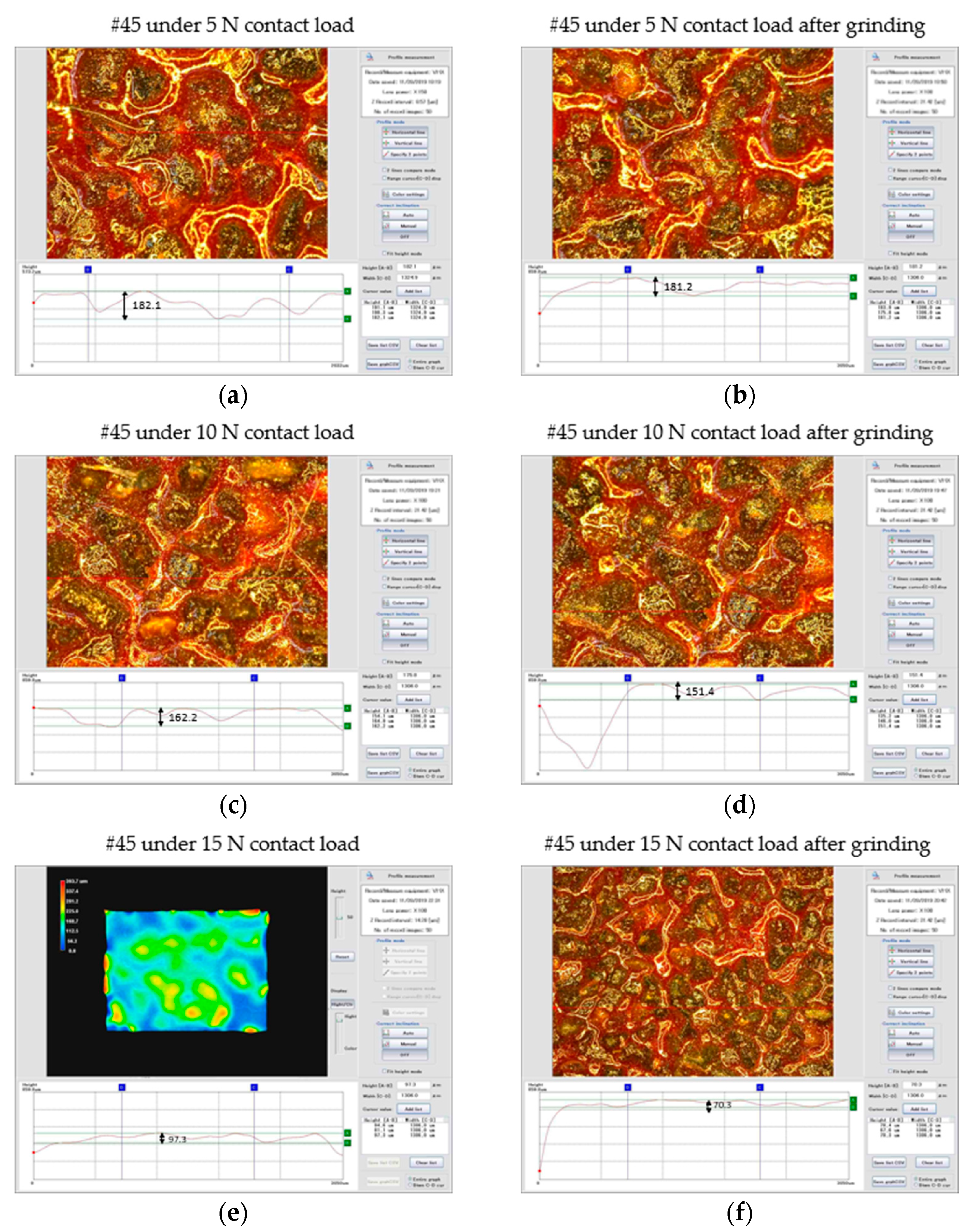
| #45 under 5 N contact load | #45 under 5 N contact load after grinding | ||||
| 191.1 | 198.3 | 182.1 | 183.9 | 175.8 | 181.2 |
| #45 under 10 N contact load | #45 under 10 N contact load after grinding | ||||
| 154.1 | 164.9 | 162.2 | 135.2 | 146.0 | 151.4 |
| #45 under 15 N contact load | #45 under 15 N contact load after grinding | ||||
| 94.6 | 81.1 | 97.3 | 78.4 | 67.6 | 70.3 |
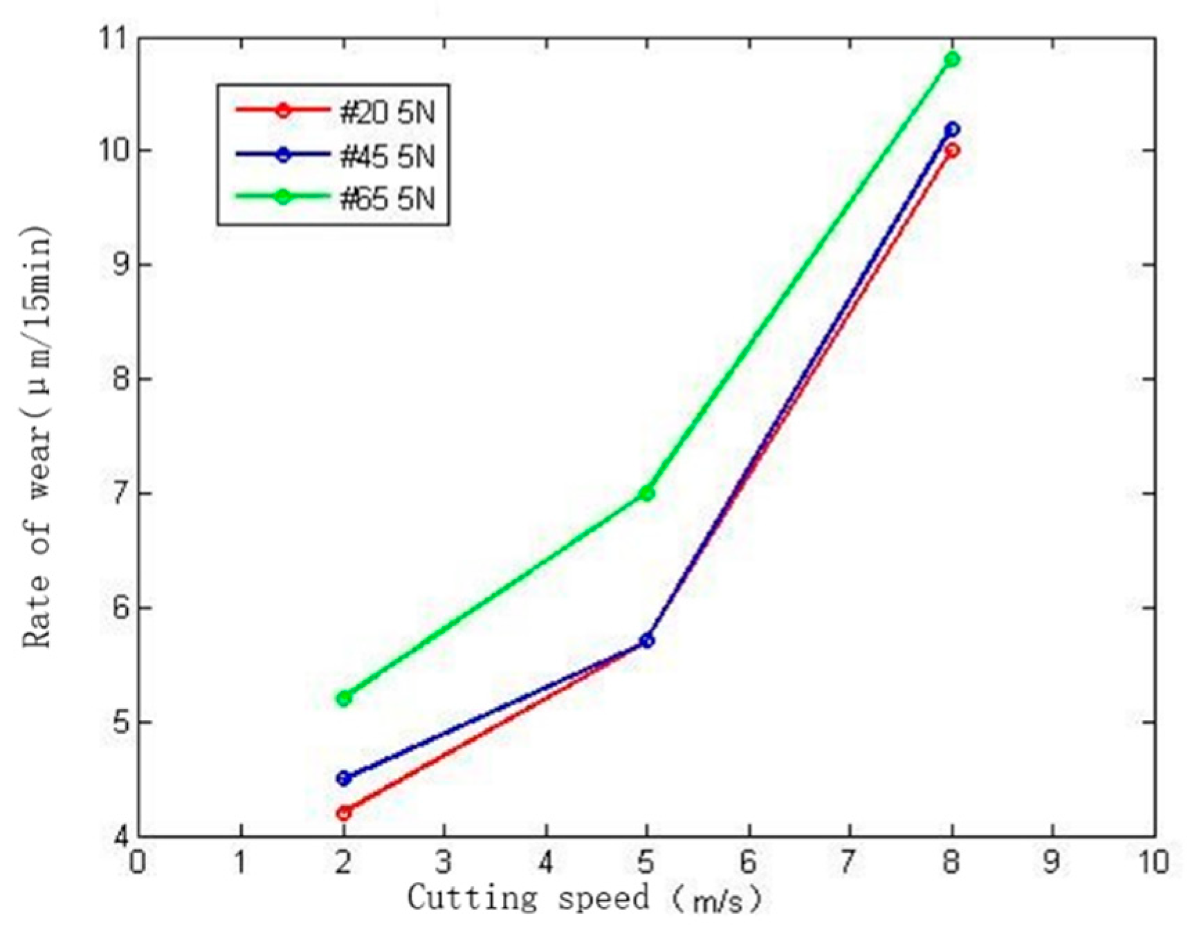
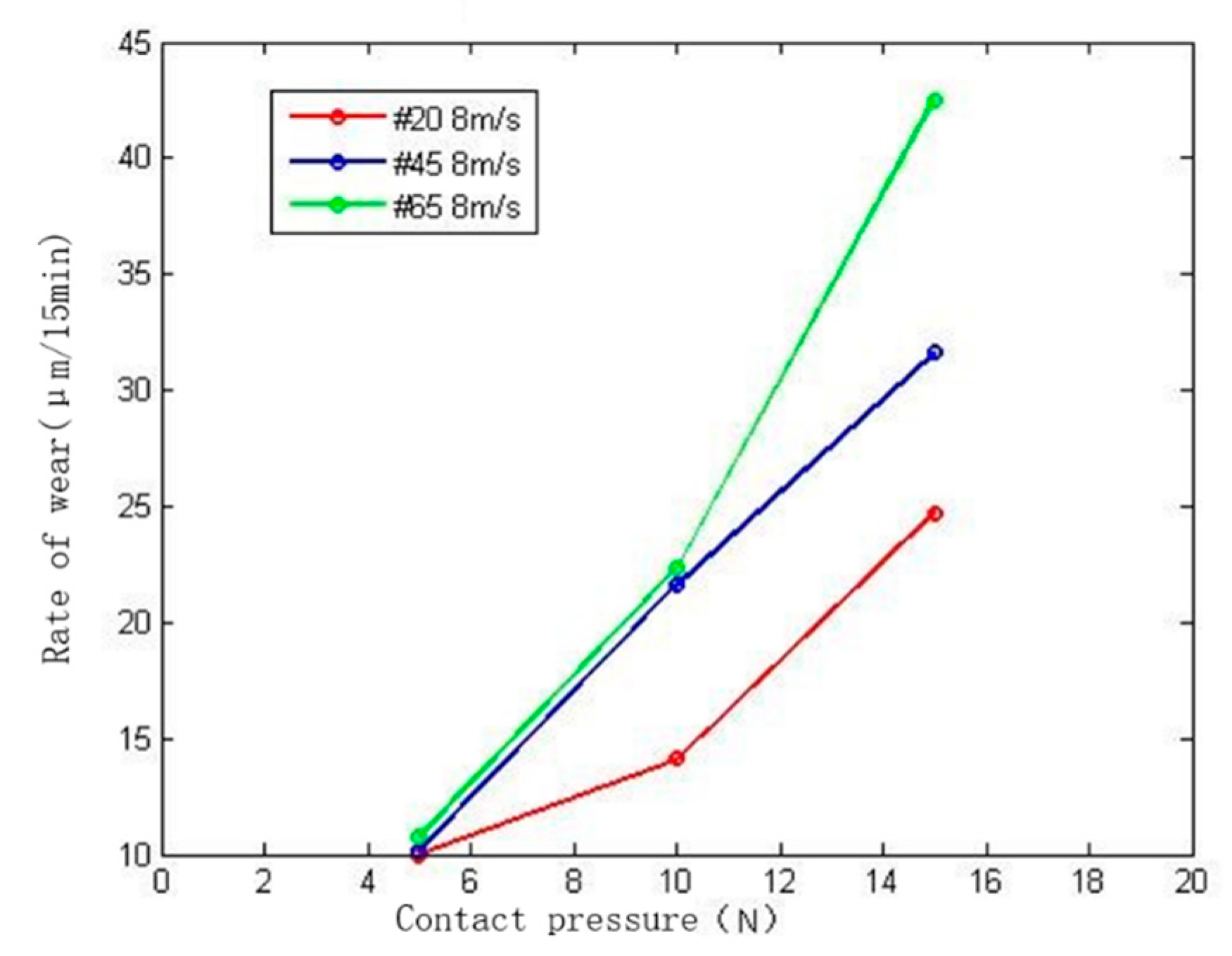
| Number | 1 | 2 | 3 | 4 | 5 | 6 | 7 | 8 | 9 |
| Δh | 10.0 | 5.7 | 4.2 | 7.6 | 10.2 | 14.1 | 24.7 | 17.1 | 8.9 |
| Number | 10 | 11 | 12 | 13 | 14 | 15 | 16 | 17 | 18 |
| Δh | 10.2 | 5.7 | 4.5 | 9.7 | 12.6 | 21.6 | 31.6 | 18.9 | 9.8 |
| Number | 19 | 20 | 21 | 22 | 23 | 24 | 25 | 26 | 27 |
| Δh | 10.8 | 7.0 | 5.2 | 10.1 | 16.5 | 22.3 | 42.5 | 28.4 | 19.0 |
| L | Training Accuracy | L | Training Accuracy |
|---|---|---|---|
| 3 | 0.21 | 8 | 0.23 |
| 4 | 0.24 | 9 | 0.20 |
| 5 | 0.11 | 10 | 0.20 |
| 6 | 0.14 | 11 | 0.21 |
| 7 | 0.16 |
| Number | 1 | 2 | 3 | 4 | 5 | 6 | 7 | 8 | 9 |
|---|---|---|---|---|---|---|---|---|---|
| Predicted result (μm) | 12.1 | 23.9 | 28.5 | 8.2 | 34.5 | 6.3 | 17.7 | 27.7 | 5.9 |
| True value (μm) | 9.9 | 19.1 | 28.3 | 10.2 | 31.3 | 9.8 | 18.8 | 24.6 | 4.3 |
| Error | 0.22 | 0.25 | 0.01 | 0.20 | 0.10 | 0.36 | 0.06 | 0.13 | 0.37 |
Publisher’s Note: MDPI stays neutral with regard to jurisdictional claims in published maps and institutional affiliations. |
© 2021 by the authors. Licensee MDPI, Basel, Switzerland. This article is an open access article distributed under the terms and conditions of the Creative Commons Attribution (CC BY) license (https://creativecommons.org/licenses/by/4.0/).
Share and Cite
Cao, Y.; Zhao, J.; Qu, X.; Wang, X.; Liu, B. Prediction of Abrasive Belt Wear Based on BP Neural Network. Machines 2021, 9, 314. https://doi.org/10.3390/machines9120314
Cao Y, Zhao J, Qu X, Wang X, Liu B. Prediction of Abrasive Belt Wear Based on BP Neural Network. Machines. 2021; 9(12):314. https://doi.org/10.3390/machines9120314
Chicago/Turabian StyleCao, Yuanxun, Ji Zhao, Xingtian Qu, Xin Wang, and Bowen Liu. 2021. "Prediction of Abrasive Belt Wear Based on BP Neural Network" Machines 9, no. 12: 314. https://doi.org/10.3390/machines9120314
APA StyleCao, Y., Zhao, J., Qu, X., Wang, X., & Liu, B. (2021). Prediction of Abrasive Belt Wear Based on BP Neural Network. Machines, 9(12), 314. https://doi.org/10.3390/machines9120314