A New Hybrid Ensemble Deep Learning Model for Train Axle Temperature Short Term Forecasting

Abstract

The axle temperature is an index factor of the train operating conditions. The axle temperature forecasting technology is very meaningful in condition monitoring and fault diagnosis to realize early warning and to prevent accidents. In this study, a data-driven hybrid approach consisting of three steps is utilized for the prediction of locomotive axle temperatures. In stage I, the Complementary empirical mode decomposition (CEEMD) method is applied for preprocessing of datasets. In stage II, the Bi-directional long short-term memory (BILSTM) will be conducted for the prediction of subseries. In stage III, the Particle swarm optimization and gravitational search algorithm (PSOGSA) can optimize and ensemble the weights of the objective function, and combine them to achieve the final forecasting. Each part of the combined structure contributes its functions to achieve better prediction accuracy than single models, the verification processes of which are conducted in the three measured datasets for forecasting experiments. The comparative experiments are chosen to test the performance of the proposed model. A sensitive analysis of the hybrid model is also conducted to test its robustness and stability. The results prove that the proposed model can obtain the best prediction results with fewer errors between the comparative models and effectively represent the changing trend in axle temperature.

1. Introduction

The reliability and efficient operation of the trains has a vital influence on the railway systems because of the continuous increase of railway transport demand. The approaches applied for railway vehicle safety monitoring have attracted much attention to the developing trend of modern railways [1]. The axle performance of the bogies in railway vehicles is essential to maintain the safety of railway transportation. The abnormal thermal failure of the axles and bearings in the bogies may bring potential risks to driving safety and the operation of the railway vehicles. As an effective indicator to reflect the condition of the axles, the research on the axle and bearing temperature monitoring and fault diagnosis can effectively ensure the safety of locomotives and can improve the management level of the railway for significant economic benefits [2]. The bearings have a certain temperature fluctuation range under normal conditions. When faults occur, the increased vibration and friction of the bearings will accumulate the generated heat, resulting in a higher temperature than the normal range, so the temperature can be used as an indicator to determine whether the bearing is under normal conditions. When the axles are damaged, it may lead to accidents of the cut axle, hot axle, or even train derailment [3]. Mostly, the axle temperature is measured and controlled by the real-time monitoring and alarm equipment and the classified information will be transmitted by the sensors to achieve an early warning over the limits for further decision-making [4,5]. In response to the demand, many axle temperature monitoring systems have been developed for the research direction. Bing et al. [6] improved restriction from the debugging methods and developed the non-destructive embedded method for EMU with axle temperature compensation as adjustment. Vale et al. [7] proposed the on-board condition monitoring system, including temperature and other factors with different types of sensors to explore the fault for early warning. Liu [8] presented an axle temperature monitoring system with an onboard switched Ethernet, connecting temperature sensors in the axle boxes for the fault diagnosis of high-speed trains. The abovementioned temperature detecting method could obtain the real-time monitoring of the axle temperature, but these methods cannot predict the changing trend of the temperatures, which is more helpful to conduct preventive measures and to avoid unnecessary loss of equipment maintenance. In recent years, researchers have put forward many prediction methods in the research field of fault diagnosis [9,10], temperature forecasting [11,12,13], wind speed forecasting [14], power forecasting [15,16], traffic flow prediction [17,18], air pollutant forecasting [19] and so on. Hence, it is meaningful to apply effective data-driven approaches to the axle temperatures for real-time status detection and prediction.

1.1. Related Work

The time series prediction approaches have been commonly applied for statistical application in the scientific study of fault diagnosis. The multiple linear regression is a widely used time series prediction method and the relevant factors are analyzed and compared by regression diagnosis to get the possible trend as the verification for the applicability of the model in temperature prediction [20]. Ma et al. [3] used the stepwise regression analysis to handle the axle temperature data. The stepwise regression analysis can input the independent variables into the regression equation, in which the original temperature data and other relevant factors are collected by sensors in high-speed trains. The results showed that the model improved resulted in short-term forecasting contributed to showing the potential trend of the original temperature dataset. From the application, it can be found that the statistical model still requires stable time series data and has difficulty in dealing with non-stationary data for information extraction.

In recent years, machine learning algorithms and artificial intelligence have attracted more attention, with the significant development and the new computing platforms which have also provided new perspectives for the predictive approaches. To further improve the accuracy, scholars have recently established many models, mainly including the statistical methods, machine learning methods, and hybrid methods [19,21]. The hybrid methods combine machine learning methods and data processing methods to provide more satisfactory prediction accuracy than single predictors [22].

The trains are running at non-uniform speed, which leads to the collected original non-stationary axle temperature. To reduce the irregular undulations of the raw datasets, the data processing methods like the decomposing methods are applied to analyze non-stationary and nonlinear processes, which could differentiate the interior features of overlapping and complex data. Wang et al. [23] utilized the Empirical mode decomposition (EMD) to decompose original datasets. Then the preprocessed results would be input to the ARIMA. The proposed model has increased the accuracy compared to single predictors. Bai et al. [24] proposed the EEMD-LSTM model for time series predictions, showing the satisfying improvement by the ensemble empirical mode decomposition (EEMD) and a successful attempt to enhance the LSTM predictor, thus reducing the complexity of the raw datasets. Chang et al. [25] applied the complementary ensemble empirical mode decomposition method (CEEMD) to preprocess and extract the remaining useful life of lithium-ion battery data. The practice proved that the CEEMD had good applicability to preprocess the non-stable datasets and extract characteristic information effectively. Considering the above analysis, the CEEMD is chosen to handle the raw data in the paper.

The predictors are the key parts of hybrid models. With the better nonlinear fitting ability, the neural network methods and deep learning methods have been widely applied in hybrid models in time series prediction. The deep learning algorithms contain a complex learning structure, in which the hidden layers lead to better learning accuracy by massive data than the statistical methods and traditional machine learning methods. Hao and Liu [26] proposed the Back Propagation Neural Network (BPNN) in the axle temperature prediction for high-speed trains. The comparative results have proved that the forecasting error of BPNN is lower than the GM (1,1) model. Yang et al. [11] presented an intelligent forecasting structure based on the Long Short-Term Memory (LSTM) for high-speed trains during operation. In the training process, a mean squared error (MSE) is used as the loss function with batch size 100 and the learning rate 0.0001. It was proved to be a feasible solution where the prediction error is arranged within a reasonable range. Luo et al. [12] also provided the LSTM-based method to predict the locomotive axle temperature based on sensor data, and the forecasting framework provided a referable result with acceptable error levels. However, the LSTM structure only inputs information in one direction. A better solution, as presented by the former study, is the BILSTM method, which is suitable for time series data and raises prediction accuracy. Zhang et al. [27] used the BILSTM to establish the hybrid time series prediction model. The experimental results indicated that the proposed BILSTM had good robustness and accuracy between the comparative models in time series prediction. The BILSTM model can use the non-linearity of series to extract deep information and to identify the characteristics of datasets. As an improved vision of LSTM, the BILSTM is applied as the time series predictor in this study.

The optimization algorithms with hybridized techniques can bring further optimization of the raw data and the prediction accuracy besides the decomposition methods and predictors. Kouchami et al. [28] designed a GA-ANN model, in which the ANN is optimized by the genetic algorithm. Xing et al. [29] used the modified grey wolf optimization (MGWO) to determine the deep belief network (DBM) structure parameters. Singh [30] combined the particle swarm optimization (PSO) algorithm with neutrosophic set theory. It was evaluated with the benchmark datasets and the hybrid model obtained improved forecasting accuracy by employing the PSO algorithm. Zhang et al. [31] also proposed PSO to improve the initial weights and thresholds of the predictor in daily global solar radiation forecasting, combining the advantages of PSO and the BPNN. In the comparative experiments, PSO-BPNN showed better accuracy than single BPNN and statistical models. Zhu et al. [32] utilized the PSOGSA optimization algorithm, which contained the particle swarm optimization (PSO) and gravitational search algorithm (GSA). By the combination of the global search ability from PSO and the local fine search ability from GSA, PSOGSA has acquired the capability of exploitation and exploration to raise the possibility of finding the best outcome. Then, the results can be easier to reach with fast convergence speed. Furthermore, the PSOGSA algorithm aims to find the global optimum between all possible values. Therefore, it is very meaningful to study the principle and the framework of the hybrid PSOGSA algorithm and to conduct more experiments for further optimization in this paper.

Therefore, this paper utilizes the information mining ability of the decomposing methods as well as deep learning, and integrates the optimization algorithm to establish a hybrid model to achieve accurate prediction of the axle temperature. According to the above literature survey, several reviewed axle temperature forecasting models are provided in

Table 1. The reviewed axle temperature forecasting models.

Reference	Published Year	Predictors
[11]	2019	LSTM
[12]	2017	LSTM
[26]	2020	BPNN
[33]	2019	SVM

.

1.2. Novelty of the Study

The main purpose of conducting this study is the research for an effective algorithm to achieve an accurate prediction of the axle temperature of locomotive bogies. A new hybrid model based on the abovementioned algorithms is proposed for the research direction. The innovation of the research is presented as below:

(a)

The time series prediction helps with the real-time monitoring onboard and the fault diagnosis of axle temperature to ensure the train safety and efficient operation. To deal with the evolving information of axle temperature series, a time series hybrid prediction model is proposed to support short-term axle temperature forecasting for early warning. Different to the multiple regression models and physical methods in the previous study, the proposed innovative model can handle the axle temperature data and reduce the calculation complexity without a decrease in the prediction accuracy.

(b)

The decomposition algorithm could efficiently process non-stationary data from a time series. The CEEMD is applied for the first time in the original non-stationary axle temperature datasets to reduce the random fluctuations and to preprocess and decompose the raw data into multiple sub-series for digging into the primary component hidden in the raw datasets. Compared to the EMD and EEMD, problems of the mode mixing and the contamination in the signal reconstruction have been solved in CEEMD so that the information of the datasets can be better extracted to enhance the predictive ability of the predictor.

(c)

In the predictive process, the long short-term memory network is utilized to learn the characteristics of the decomposed IMFs. The improved version BILSTM can further learn long-term dependency of sequences by the deep learning structure of the evaluation of past and future information without keeping redundant characteristics [34]. It is also the first application in axle temperature prediction.

(d)

Different to other statistical computation or neural network methods, the proposed model is an ensemble predicting method focusing on the new hybrid metaheuristic optimization algorithm PSOGSA, which takes advantage of the exploitation function from PSO and the exploration function from GSA. The hybrid algorithm used each subsequence prediction result matrix from CEEMD-BILSTM and the weight matrix to find the optimal solution in the objective function and combine the calculation results for output.

(e)

The proposed hybrid CEEMD-BILSTM-PSOGSA is a novel structure. Recently, many applied forecasting models of the axle temperature have been single predictors. Therefore, the combining performance of hybrid models and the ability of the single models are worth studying. To test the robustness and accuracy and to evaluate the total performance, the experiments were conducted as the benchmark test.

2. Methodology

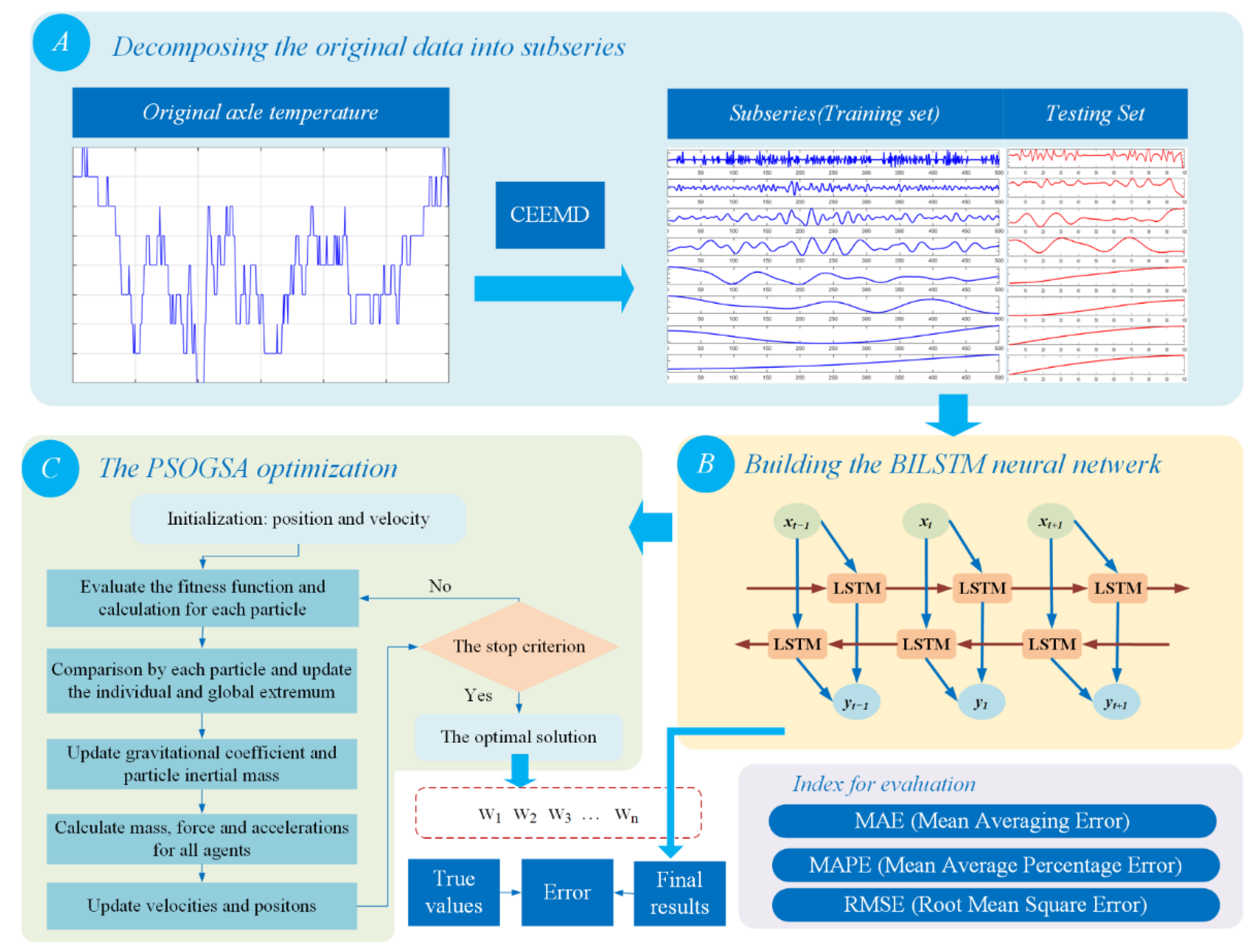
2.1. The Overall Structure of the Axle Temperature Forecasting Model

The structure of the proposed hybrid model is shown in Figure 1, including the decomposition methods, the deep learning predictor, and the ensemble learning methods. The detailed process is demonstrated as follows:

Part A: The original axle temperature series are decomposed by the CEEMD method into several subseries separately, which could decrease the non-stationarity of the model for further optimization in the next step. The raw temperature data can be separated and applied as the training set and testing set. The input data can be trained in the training set and then the total performance of the optimal model will be tested by the testing set. The detailed explanations of CEEMD are shown in Section 2.2.

Part B: The BILSTM, a combination of forward LSTM and backward LSTM, will be conducted to obtain the prediction results for the sub-series after the process of CEEMD. The deep network receives the forecasting results by combining all the forecasting results from the sub-series. The principles of the BILSTM are shown in Section 2.3.

Part C: The PSOGSA is applied to optimize and ensemble the weights of the objective function in model training. The PSOGSA can analyze the features of sub-series results and optimize the weight coefficients of the decomposed subseries. Then, the sub-results from each model should be integrated by the corresponding weights (w₁, w₂…w_n) to obtain the final predictive data. The formula is shown as follows:

$$\widehat{\mathrm{A}}(\mathrm{t})={\mathrm{w}}_1{\widehat{\mathrm{A}}}_1(\mathrm{t})+{\mathrm{w}}_2{\widehat{\mathrm{A}}}_2(\mathrm{t})+\cdots +{\mathrm{w}}_{\mathrm{n}}{\widehat{\mathrm{A}}}_{\mathrm{n}}(\mathrm{t})$$

(1)

where w_i are the weight coefficients, ${\widehat{\mathrm{A}}}_{\mathrm{i}}(\mathrm{t})$ are the prediction results of each sub-series. The product of each subsequent prediction result matrix and the weight matrix will be compared to the raw data to get the satisfying results, which are evaluated by the indexes. The principles of the PSOGSA are shown in Section 2.4.

2.2. Complementary Ensemble Empirical Mode Decomposition Method

As an important member in a series of data preprocessing approaches based on EMD, the CEEMD was proposed by Yeh et al. [35] to develop the EMD and the ensembled EMD (EEMD) decomposition methods. The EMD can decompose raw complicated data adaptively into a group of intrinsic mode functions (IMFs) [36]. However, the method also presents mode mixing that a single IMF signal may contain different time scales or at the same time scale appears in different IMFs. The EEMD was designed to eliminate the mode mixing problem [37]. They added the normally distributed white noise to the raw signal and then performed EMD decomposition to acquire each IMF. However, EEMD still has the problem of contamination in the data reconstruction. To solve the problem that the white noise cannot be completely removed after reconstruction, and because the noise is too large after the addition, CEEMD was proposed and widely used. In addition to reducing the mode mixing, the CEEMD also eliminates the final white noise residual and raises the calculated efficiency. The main process of the CEEMD is briefly summarized below:

Step 1: The raw signal y(t) has a plus of opposite white noises to produce new signals with positive and negative noises separately [38], and the new signals are:

$$\{\begin{array}{l}{\mathrm{y}}_{\mathrm{i}}^{+}(\mathrm{t})=\mathrm{y}(\mathrm{t})+{\mathrm{w}}_{\mathrm{i}}(\mathrm{t})\\ {\mathrm{y}}_{\mathrm{i}}^{-}(\mathrm{t})=\mathrm{y}(\mathrm{t})-{\mathrm{w}}_{\mathrm{i}}(\mathrm{t})\end{array}$$

(2)

where w_i(t) is the ith plus white noise, ${\mathrm{y}}_{\mathrm{i}}^{+}(\mathrm{t})$ and ${\mathrm{y}}_{\mathrm{i}}^{-}(\mathrm{t})$ represent the ith positive and negative signals.

Step 2: The new signals ${\mathrm{y}}_{\mathrm{i}}^{+}(\mathrm{t})$, ${\mathrm{y}}_{\mathrm{i}}^{-}(\mathrm{t})$ are separated into two sets of IMFs by the EMD method,

$$\{\begin{array}{l}{\mathrm{y}}_{\mathrm{i}}^{+}(\mathrm{t})={\displaystyle \sum _{\mathrm{j}=1}^{\mathrm{m}}{\mathrm{d}}_{\mathrm{i}\mathrm{j}}^{+}}(\mathrm{t})\\ {\mathrm{y}}_{\mathrm{i}}^{-}(\mathrm{t})={\displaystyle \sum _{\mathrm{\text{j}}=1}^{\mathrm{m}}{\mathrm{\text{d}}}_{\mathrm{i}\mathrm{j}}^{-}}(\mathrm{t})\end{array}$$

(3)

where ${\mathrm{y}}_{\mathrm{i}}^{+}(\mathrm{t})$, and ${\mathrm{y}}_{\mathrm{i}}^{-}(\mathrm{t})$ represent the jth IMFs obtained in the ith time with positive and negative noise, m is the number of IMFs.

Step 3: Repeat steps 1 and 2 N times with varying sizes of white noises in each time to get IMF components.

Step 4: Get the ensemble average of all the relative IMFs, described as:

$${\mathrm{d}}_{\mathrm{j}}(\mathrm{t})=\frac{1}{2\mathrm{N}}{\displaystyle \sum _{\mathrm{i}=1}^{\mathrm{N}}\left({\mathrm{\text{d}}}_{\mathrm{i}\mathrm{j}}^{+}(\mathrm{t})+{\mathrm{\text{d}}}_{\mathrm{i}\mathrm{j}}^{-}(\mathrm{t})\right)}$$

(4)

where d_j(t) is the jth IMF item obtained by the CEEMD method.

Step 5: After step 4, when there are not more than two peaks in the remainder ${\mathrm{r}}_{\mathrm{N}}(\mathrm{t})=\mathrm{y}(\mathrm{t})-{\displaystyle {\sum }_{\mathrm{j}=1}^{\mathrm{N}}{\mathrm{d}}_{\mathrm{j}}(\mathrm{t})}$, the step is finished and conducted the next step. If not, begin steps 1–4 again [39].

Step 6: The raw signal y(t) can be concluded as:

$$\mathrm{y}(\mathrm{t})={\displaystyle \sum _{\mathrm{j}=1}^{\mathrm{N}}{\mathrm{d}}_{\mathrm{j}}(\mathrm{t})+{\mathrm{r}}_{\mathrm{N}}(\mathrm{t})}$$

(5)

where d_j(t) is the jth IMF and r_N(t) is the remainder.

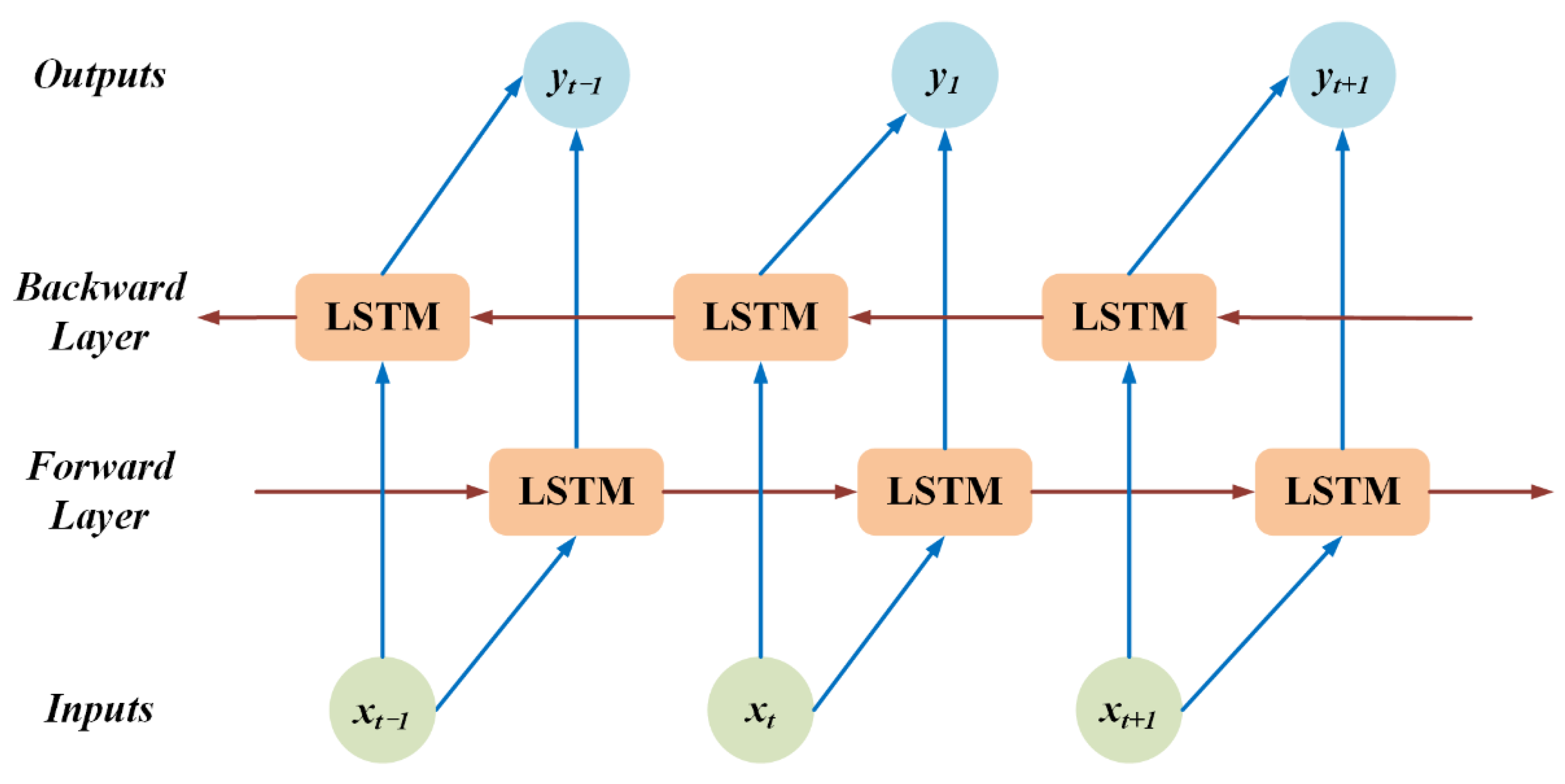
2.3. Bi-Directional Long Short-Term Memory Method

The LSTM belongs to the recurrent neural network and it was proposed in 1997 [40]. Due to the characteristics of its design, LSTM is very appropriate for modeling time series data. Compared with other recurrent neural networks, LSTM networks provide the application of the threshold structure to selectively retain or forget relevant information. An LSTM unit has three gate structures, including the input gate, the output gate, and the forget gate [41]. The gating units are responsible for controlling the information flow as an interface [42]. In the learning process, the weight can be renovated automatically [43]. The input and forget gates determine the data which should be added or removed and the output gate determines the parts of the output. The structure of LSTM is shown in Figure 2. The process of LSTM is expressed as the following steps with the notations [42]:

▪

i_t, f_t, and o_t are respectively vectors for the input gate, forget gate, and output gate.

▪

r_t and ${\tilde{\mathrm{r}}}_{\mathrm{t}}$ are the cell status and the values vectors.

▪

x_t is the input data and h_t is the output variable.

▪

w_cx, w_ix, w_fx, w_ox, w_ch, w_ih, w_fh, w_oh represent the relative weight matrices.

▪

b_i, b_r, b_f, b_o are the relative bias vectors and σ is a sigmoid activation function.

Step 1: The LSTM layer obtains the information from its last cell states r_t−1. The input x_t, the previous output h_t−1, and the bias terms b_f of the forget gates are used for calculating the activation values f_t by a sigmoid activation function σ [44].

$${\mathrm{f}}_{\mathrm{t}}=\sigma ({\mathrm{w}}_{\mathrm{f}\mathrm{x}}{\mathrm{x}}_{\mathrm{t}}+{\mathrm{w}}_{\mathrm{f}\mathrm{h}}{\mathrm{h}}_{\mathrm{t}-1}+{\mathrm{b}}_{\mathrm{f}})$$

(6)

Step 2: The LSTM layer determines the new data to be stored and then calculates the data to be transferred to the network.

$${\tilde{\mathrm{r}}}_{\mathrm{t}}=\tanh ({\mathrm{w}}_{\mathrm{c}\mathrm{x}}{\mathrm{x}}_{\mathrm{t}}+{\mathrm{w}}_{\mathrm{c}\mathrm{h}}{\mathrm{h}}_{\mathrm{t}-1}+{\mathrm{b}}_{\mathrm{r}})$$

(7)

$${\mathrm{i}}_{\mathrm{t}}=\sigma ({\mathrm{w}}_{\mathrm{i}\mathrm{x}}{\mathrm{x}}_{\mathrm{t}}+{\mathrm{w}}_{\mathrm{i}\mathrm{h}}{\mathrm{h}}_{\mathrm{t}-1}+{\mathrm{b}}_{\mathrm{i}})$$

(8)

Step 3: Take the outcome in the above process to acquire new call status r_t and the ∘ means the Hadamard product.

$${\mathrm{r}}_{\mathrm{t}}={\mathrm{f}}_{\mathrm{t}}\circ {\mathrm{r}}_{\mathrm{t}-1}+{\mathrm{i}}_{\mathrm{t}}\circ {\tilde{\mathrm{r}}}_{\mathrm{t}}$$

(9)

Step 4: the output h_t of the LSTM layer by the following calculations:

$${\mathrm{o}}_{\mathrm{t}}=\sigma ({\mathrm{w}}_{\mathrm{o}\mathrm{x}}{\mathrm{x}}_{\mathrm{t}}+{\mathrm{w}}_{\mathrm{o}\mathrm{h}}{\mathrm{h}}_{\mathrm{t}-1}+{\mathrm{b}}_{\mathrm{o}})$$

(10)

$${\mathrm{h}}_{\mathrm{t}}={\mathrm{o}}_{\mathrm{t}}\circ \tanh ({\mathrm{r}}_{\mathrm{t}})$$

(11)

The BILSTM is short for Bi-directional Long Short-Term Memory and it is architecturally composed of forwarding LSTM and backward LSTM [45]. Similar to LSTM, both are often used to model context information in natural language processing tasks [42]. The BILSTM can connect two hidden layers with different directions to output, which means it includes forward and backward data at the same time. The BILSTM can raise LSTM model performance in classification processes and effectively learn long-term dependency. The output layer can get past and future information in the input data by the structure. The structure of the BILSTM network is expressed in Figure 3.

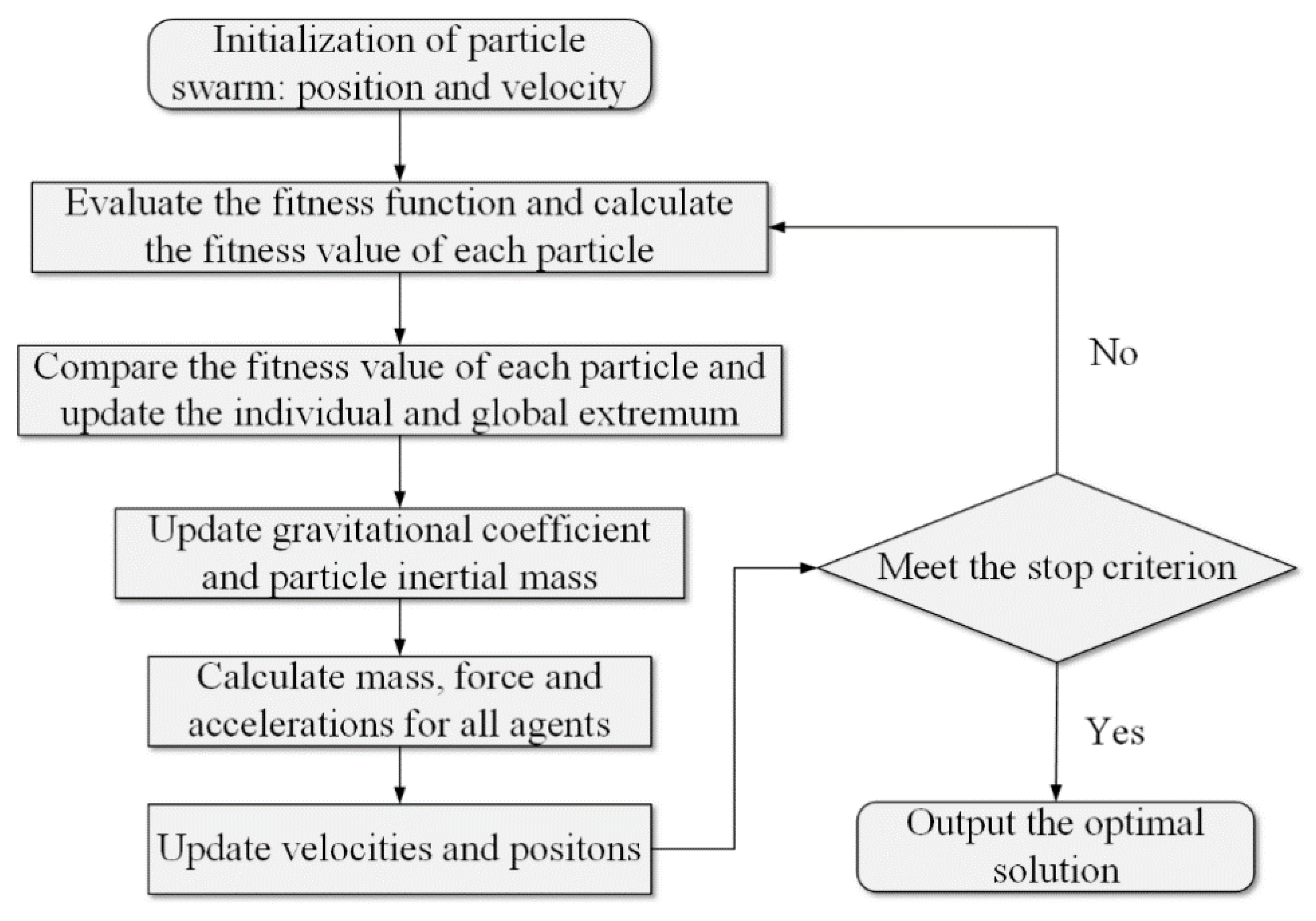
2.4. Ensemble Learning Method Based on PSOGSA Optimization

Kennedy and Eberhart [46] proposed the concept of the position and velocity-based meta-heuristic algorithm PSO in 1995, which searches for the optimal value by simulating the foraging behavior of birds. The PSO algorithm is popular for its efficiency to converge to the optimum value and its special characteristics takes advantage of both the individual and group information to adjust status. Finally, it could have a fast speed to an optimal value.

The PSO draws inspiration from this phenomenon to conduct optimization. In the PSO algorithm, the potential result to the optimal problem is similar to a bird in the search area. All particles start with a fitness value decided by the optimized function [39]. They also have a speed according to the direction and distance they move, and move along the current best particle and search for the optimal solution through multiple iterations, in which the particle updates by the individual extremum pbest and the optimal value from the entire group as the global extremum gbest [47]. It can also update with the extreme values of the neighbors of the particle as local extreme values [48]. The equations of the PSO is expressed as follows:

$${\mathrm{v}}_{\mathrm{i}}(\mathrm{t}+1)=\mathrm{w}\times {\mathrm{v}}_{\mathrm{i}}(\mathrm{t})+{\mathrm{d}}_1\times \mathrm{r}\mathrm{a}\mathrm{n}\mathrm{d}\times ({\mathrm{pbest}}_{\mathrm{i}}-{\mathrm{x}}_{\mathrm{i}}(\mathrm{t}))+{\mathrm{d}}_2\times \mathrm{r}\mathrm{a}\mathrm{n}\mathrm{d}\times (\mathrm{gbest}-{\mathrm{x}}_{\mathrm{i}}(\mathrm{t}))$$

(12)

$${\mathrm{x}}_{\mathrm{i}}(\mathrm{t}+1)={\mathrm{x}}_{\mathrm{i}}(\mathrm{t})+{\mathrm{v}}_{\mathrm{i}}(\mathrm{t}+1)$$

(13)

where v_i is the velocity, x_i(t) represents the current location of ith particle, t means iteration, w represents the weight, d₁ and d₂ are the acceleration coefficients. rand means a uniform random variable between the interval [0, 1]. pbest represents the local best location of ith particle, and gbest has been defined as the global optimal result [48].

The gravitational search algorithm (GSA) was originally designed in 2009 [49]. It is based on the law of universal gravitation and Newton’s second law. The GSA can lead the group to conduct an optimization search by the universal gravity between the particles in the entire population. Taking advantage of GSA’s strong global optimization ability and the feature that PSO can increase memory and social information exchangeability for particles, Mirjalili and Hashim [50] proposed a hybrid algorithm PSOGSA combined the PSO and GSA, which includes the exploration ability of PSO and the research localization ability of GSA [51]. The Figure 4 shows the schematic process of PSOGSA.

The developed velocity of PSOGSA is shown as follows:

$${\mathrm{V}}_{\mathrm{i}}(\mathrm{t}+1)={\mathrm{w}}^{\prime }\times {\mathrm{V}}_{\mathrm{i}}(\mathrm{t})+{\mathrm{d}}_1^{\prime }\times \mathrm{r}\mathrm{a}\mathrm{n}\mathrm{d}\times \mathrm{a}{\mathrm{c}}_{\mathrm{i}}(\mathrm{t})+{\mathrm{d}}_{{}_2}^{\prime }\times \mathrm{r}\mathrm{a}\mathrm{n}\mathrm{d}\times (\mathrm{gbest}-{\mathrm{X}}_{\mathrm{i}}(\mathrm{t}))$$

(14)

$${\mathrm{X}}_{\mathrm{i}}(\mathrm{t}+1)={\mathrm{X}}_{\mathrm{i}}(\mathrm{t})+{\mathrm{V}}_{\mathrm{i}}(\mathrm{t}+1)$$

(15)

where V_i is the velocity, X_i(t) represents the current location of the ith particle. t is the iteration, w’ is the weight, ${\mathrm{d}}_1^{\prime }$ and ${\mathrm{d}}_2^{\prime }$ are the acceleration coefficients. rand represents a random variable between the interval [0, 1]. ac_i(t) means the acceleration of the ith agent. The gbest means the current best result and v_i represents the velocity of the ith agent [48].

In the study, the mean square error is applied as the objective function,

$$\mathrm{MSE}=({\displaystyle \sum _{\mathrm{t}=1}^{\mathrm{N}}{\left[\mathrm{A}(\mathrm{t})-\widehat{\mathrm{A}}(\mathrm{t})\right]}^2)/\mathrm{n}}$$

(16)

where $\mathrm{A}(\mathrm{t})$ means the raw data, $\widehat{\mathrm{A}}(\mathrm{t})$ represents the predictive result and n is the number of samples in  $\mathrm{\text{A}}(\mathrm{t})$.

For the n decomposed sub-series from CEEMD, the state matrix S can be presented as the weight matrix,

$$\mathrm{S}=\left[{\mathrm{w}}_1,{\mathrm{w}}_2\dots {\mathrm{w}}_{\mathrm{n}}\right]$$

(17)

where w₁, w₂…w_n are the corresponding weights and n represents the number of the decomposed sub-series from CEEMD. The product of the prediction result matrix and the weight matrix will be compared to the raw data by the optimization algorithm for fulfilling results in the objective function. The iteration ends up with a fulfilling condition. The test set is inputted into the trained model and the PSOGSA determines the optimal weights by the data features of the test set.

3. Case Study

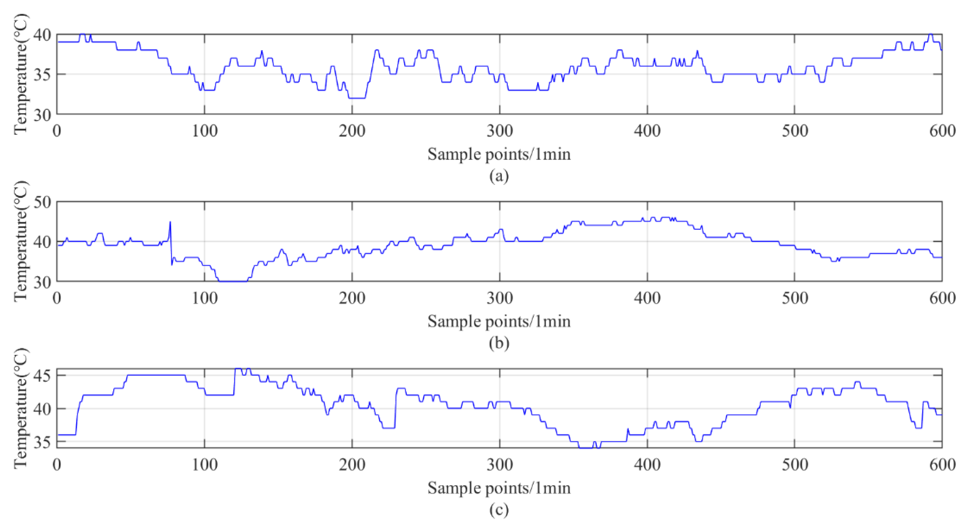
3.1. The Applied Datasets

In the research, the raw collected data are applied to verify the performance of the proposed hybrid model. The temperature datasets #1, #2, and #3 were measured with a 1-min interval by different axles in the Harmony diesel locomotive. The original data are displayed in Figure 5 with 600 sample points in each subseries. As a description of the datasets,

Table 2. Dataset description.

Dataset	Maximum (°C)	Minimum (°C)	Average (°C)
1	40	32	35.9317
2	46	30	39.0567
3	46	34	40.4950

lists the maximum, minimum, and average values of the three datasets. According to the literature survey [14,52,53] of prediction models, the proportion of training set and testing set can be 5:1 to 7:1. In the paper, each series includes 600 samples, in which the training set has 500 samples for the predictor and the testing set includes 100 samples to test the accuracy of the models. All experiments are supported by the Matlab2020a platform.

3.2. The Evaluation Indexes in the Study

The evaluation indexes are necessary to assess the model performance. In this paper, the indexes have been utilized, which are the mean absolute error (MAE), the mean absolute percentage error (MAPE), and the root mean square error (RMSE). Moreover, the promoting percentages (P_MAE, P_MAPE, P_RMSE) are also utilized in the study for a further comparison between the models. The indexes are expressed as follows:

$$\{\begin{array}{l}\mathrm{MAE}=({\displaystyle \sum _{\mathrm{t}=1}^{\mathrm{n}}\left|\mathrm{A}(\mathrm{t})-\widehat{\mathrm{A}}(\mathrm{t})\right|})/\mathrm{n}\\ \mathrm{MAPE}=({\displaystyle \sum _{\mathrm{t}=1}^{\mathrm{n}}\left|(\mathrm{A}(\mathrm{t})-\widehat{\mathrm{A}}(\mathrm{t}))/\mathrm{A}(\mathrm{t})\right|})/\mathrm{n}\\ \mathrm{RMSE}=\sqrt{({\displaystyle \sum _{\mathrm{t}=1}^{\mathrm{n}}{\left[\mathrm{A}(\mathrm{t})-\widehat{\mathrm{A}}(\mathrm{t})\right]}^2)/\mathrm{n}}}\end{array}$$

(18)

$$\{\begin{array}{l}{\mathrm{P}}_{\mathrm{MAE}}=\left({\mathrm{MAE}}_{\mathrm{a}}-{\mathrm{MAE}}_{\mathrm{b}}\right)/{\mathrm{MAE}}_{\mathrm{a}}\\ {\mathrm{P}}_{\mathrm{MAPE}}=\left({\mathrm{RAPE}}_{\mathrm{a}}-{\mathrm{MAPE}}_{\mathrm{b}}\right)/{\mathrm{MAPE}}_{\mathrm{a}}\\ {\mathrm{P}}_{\mathrm{RMSE}}=\left({\mathrm{RMSE}}_{\mathrm{a}}-{\mathrm{RMSE}}_{\mathrm{b}}\right)/{\mathrm{RMSE}}_{\mathrm{a}}\end{array}$$

(19)

where $\mathrm{A}(\mathrm{t})$ is the original data, $\widehat{\mathrm{A}}(\mathrm{t})$ is the predictive output and n is the number of samples in $\mathrm{A}(\mathrm{t})$.

3.3. Comparing Experiments and Results

To test the model forecasting ability, different relevant models are compared and analyzed by different indexes in the paper. The conducted experiments contain three stages.

3.3.1. Experimental Results of Part 1

As the first application in axle temperature forecasting, BILSTM is tested in experiments with other predictors, which are LSTM, DBN, ENN, BPNN, MLP, ARIMA, and ARMA models, including the aspects of neural networks, deep learning, and regression methods.

Table 3. The error evaluation results of different predictors in series #1, #2, and #3.

Series	Forecasting Models	MAE (°C)	MAPE (%)	RMSE (°C)
#1	BILSTM	0.2297	0.6159	0.3814
	LSTM	0.2702	0.7522	0.4475
	DBN	0.3673	0.8565	0.4516
	ENN	0.2814	0.7531	0.4832
	BPNN	0.2805	0.9234	0.5297
	MLP	0.5456	1.6037	0.7350
	ARIMA	0.5835	1.7129	0.8644
	ARMA	0.6326	1.9583	1.1152
#2	BILSTM	0.2568	0.6086	0.3764
	LSTM	0.2838	0.6987	0.4167
	DBN	0.3185	0.7586	0.4684
	ENN	0.3911	0.7922	0.4396
	BPNN	0.4055	1.1015	0.5007
	MLP	0.7026	1.8110	0.8988
	ARIMA	0.7941	1.9375	0.9259
	ARMA	0.9102	2.1479	1.2074
#3	BILSTM	0.3135	0.6830	0.4710
	LSTM	0.3929	0.7851	0.5490
	DBN	0.3703	0.7582	0.5784
	ENN	0.3563	0.7225	0.5739
	BPNN	0.4342	1.0436	0.6290
	MLP	0.7340	1.6931	1.0061
	ARIMA	0.9351	1.7859	1.2134
	ARMA	1.1046	1.8705	1.3743

presents the test results and Figure 6, Figure 7 and Figure 8 also show the part of the error evaluation results of the single predictors.

3.3.2. Experimental Results of Part 2

To validate the superiorities of the decomposition methods, the research lists the results of the hybrid EMD-BILSTM, EEMD-BILSTM, and CEEMD-BILSTM models. The prediction accuracy, the advantages, and the disadvantages of the decomposition algorithm are also demonstrated.

Table 4. The error evaluation results of different models in series #1, #2, and #3.

Series	Forecasting Models	MAE (°C)	MAPE (%)	RMSE (°C)
#1	BILSTM	0.2297	0.6159	0.3814
	EMD-BILSTM	0.2180	0.5987	0.3466
	EEMD-BILSTM	0.2115	0.5673	0.3092
	CEEMD-BILSTM	0.1735	0.4545	0.2797
#2	BILSTM	0.2568	0.6086	0.3764
	EMD-BILSTM	0.2329	0.5272	0.3039
	EEMD-BILSTM	0.2164	0.4802	0.2736
	CEEMD-BILSTM	0.1937	0.4628	0.2529
#3	BILSTM	0.3135	0.6830	0.4710
	EMD-BILSTM	0.2901	0.6321	0.4361
	EEMD-BILSTM	0.2831	0.5954	0.4055
	CEEMD-BILSTM	0.2511	0.5692	0.3895

and

Table 5. The promoting percentages of the EMD decomposition algorithms.

Methods	Indexes	Series #1	Series #2	Series #3
EMD-BILSTM vs. BILSTM	PMAE (%)	5.0936	9.3069	7.4641
	PMAPE (%)	2.7927	13.3750	7.4524
	PRMSE (%)	9.1243	19.2614	7.4098
EEMD-BILSTM vs. BILSTM	PMAE (%)	7.9234	15.7321	9.9697
	PMAPE (%)	7.8909	21.0976	12.8258
	PRMSE (%)	18.9303	27.3114	13.9066
CEEMD-BILSTM vs. BILSTM	PMAE (%)	24.4467	24.5717	19.9043
	PMAPE (%)	26.2056	23.9566	16.6618
	PRMSE (%)	26.6650	32.8108	17.3036

show the test results and the promoting percentages.

3.3.3. Experimental Results of Part 3

To further evaluate the performance, the proposed model is tested with other models optimized by ensemble algorithms. This experiment can prove that the superiority of the hybrid framework to other single predictors without the optimization algorithms and can demonstrate exceptional application prospects of the proposed model.

Table 6. The promoting percentages of the proposed model, the CEEMD-BILSTM and the BILSTM.

Methods	Indexes	Series #1	Series #2	Series #3
CEEMD-BILSTM-PSOGSA vs. CEEMD-BILSTM	PMAE (%)	40.8360	49.6644	51.4138
	PMAPE (%)	39.7360	54.3431	38.3345
	PRMSE (%)	33.5001	51.2456	43.7741
CEEMD-BILSTM-PSOGSA vs. BILSTM	PMAE (%)	55.0283	62.0327	61.0845
	PMAPE (%)	55.5285	65.2810	48.6091
	PRMSE (%)	51.2323	67.2423	53.5032

and

Table 7. The promoting percentages of the proposed model, the CEEMD-BILSTM-GWO model and the hybrid CEEMD-BILSTM-PSO model.

Methods	Indexes	Series #1	Series #2	Series #3
CEEMD-BILSTM-PSOGSA vs. CEEMD-BILSTM-PSO	PMAE (%)	11.9352	14.9956	15.5709
	PMAPE (%)	15.1487	18.2276	17.4118
	PRMSE (%)	16.2162	25.4534	13.7795
CEEMD-BILSTM-PSOGSA vs. CEEMD-BILSTM-GWO	PMAE (%)	21.2652	38.9480	44.5958
	PMAPE (%)	20.9067	47.7756	33.2953
	PRMSE (%)	25.5702	47.3077	33.3738

show the promoting level of the proposed CEEMD-BILSTM-PSOGSA to other models. Figure 6, Figure 7 and Figure 8 indicate the evaluation results of the eight models for different axle temperature datasets. Figure 9 presents the loss values by the iterations of PSOGSA, PSO, and GWO. Figure 10, Figure 11 and Figure 12 show the total forecasting results and errors for experiments, which describe the curve of the forecasting results in eight models with the raw data, and the error distribution and the local enlargement.

3.4. Comparison and Discussion with Alternative Algorithms

3.4.1. Analysis of Applied Single Predictors

From Table 3 and Figure 6, Figure 7 and Figure 8, it can be summarized that:

(a)

The prediction accuracies of the neural network model and deep learning models are much higher than that of ARIMA and ARMA in all the datasets. For the statistical regression methods, the high fluctuation, nonstationary and nonlinear features of axle temperature series may increase the difficulty of the prediction process and lead to low prediction accuracy. The corresponding experiment results of three datasets reflected the insufficient ability of ARIMA and ARMA methods to solve nonlinear modeling. Besides, the prediction accuracy of the MLP is lower than other deep learning models in the series. It demonstrates that the performance of the shallow neural network is not good as the deep neural network in the research. The multiple hidden layers in the deep neural networks may complete the analysis of the deep wave information of original datasets and improve training and optimization capabilities to analyze the fluctuation and nonlinear features of the temperature data. Taking advantage of the deep learning methods, they can conduct a full analysis by the continuous iteration training process to keep stable and robust in the calculation of the temperature datasets.

(b)

Comparing the results of the LSTM and other benchmarks DBN, ENN, BPNN, MLP, ARIMA, and ARMA, the prediction error of the is lower than that of others and BILSTM obtains the best prediction results in all series. In Figure 6, Figure 7 and Figure 8, the evaluation values of BILSTM are lower than the neural networks and deep networks. The difference in the figures can be found that the MAPE of BILSTM is 0.6086% and the MAPE of BPNN is 1.1015%. The possible reason may be that the bidirectional operation structure could analyze the contextual information to increase the calculation speed and recognition abilities for different data series so that the type of neural network training can acquire optimal results in axle temperature time-series forecasting. However, it can be observed that a single predictor is not enough to efficiently handle different axle temperature series. Because of the hidden layer structures from different deep networks, the recognition abilities of the deep networks for various types of time series are also varied, so that it is essential to utilize other algorithms to increase the applicability and robustness of the model.

3.4.2. Analysis of Applied Decomposition Methods

From Table 4 and Table 5 in the experimental results of Part 2, it can be found that:

(a)

The results from the EMD-BILSTM, EEMD-BILSTM and CEEMD-BILSTM models have shown better accuracy than the single BILSTM model. Therefore, the BILSTM with the decomposition algorithms has the ability to achieve better feature extraction of the axle temperature series and to produce more accurate forecasting results than the single BILSTM. Although the decomposition methods may raise the complexity and the time costs to a certain extent, considering the overall improvement effect, the application of real-time decomposition is feasible and is worthy of recognition in forecasting.

(b)

From the tables, it can be found that the forecasting errors of the EMD-BILSTM are higher than the EEMD-BILSTM and CEEMD-BILSTM in all series, which is a gradual decrease process. This application proves that the ability of the EMD method on decomposing the original signal and selecting the related partial characteristic of the original signal is lower than other models. The possible reason is that the mode mixing problem affects the processing and extraction capabilities of the EMD method for non-stationary and nonlinear data. Likewise, the signal reconstruction problem can also reduce the accuracy of the EEMD by the data decomposition, which leads to the production of white noise.

(c)

The comparable data in the tables have proved that the CEEMD is more efficient than the EMD and EEMD to raise the prediction accuracy. The CEEMD algorithm can raise sharply more than 32% of the accuracy for a single BILSTM in the forecasting results in all datasets, which can be also reflected in Figure 6, Figure 7 and Figure 8. Due to the function of improvement in eliminating the residual noise and the mode mixing, the CEEMD takes advantage of EEMD and represents a superior research potential to deepen the information extraction for temperature data.

3.4.3. Analysis of Different Optimization Methods

From Table 6 and Table 7 and Figure 6, Figure 7, Figure 8, Figure 9, Figure 10, Figure 11 and Figure 12 in experimental results of Part 3, it can be demonstrated that:

(a)

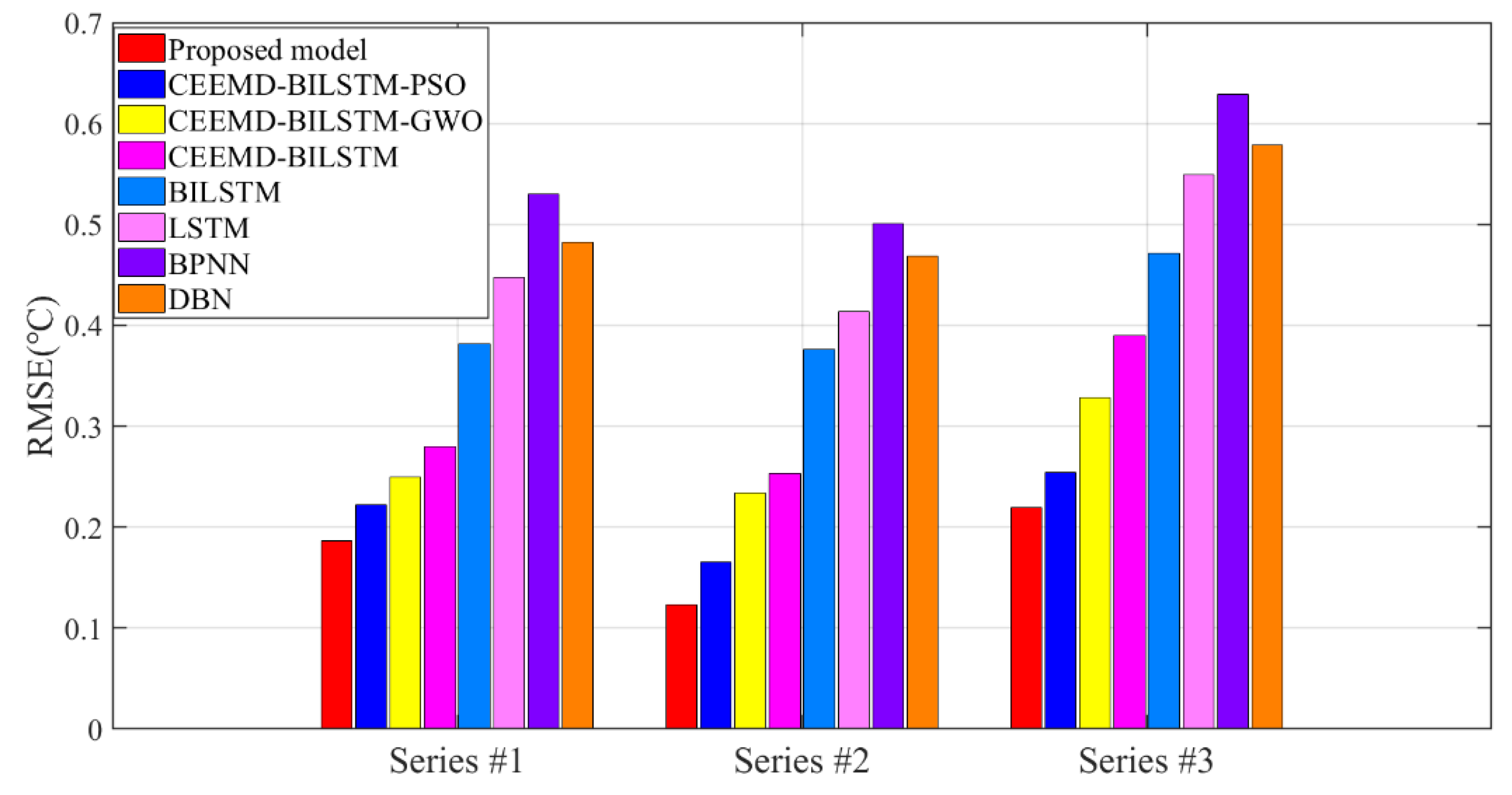
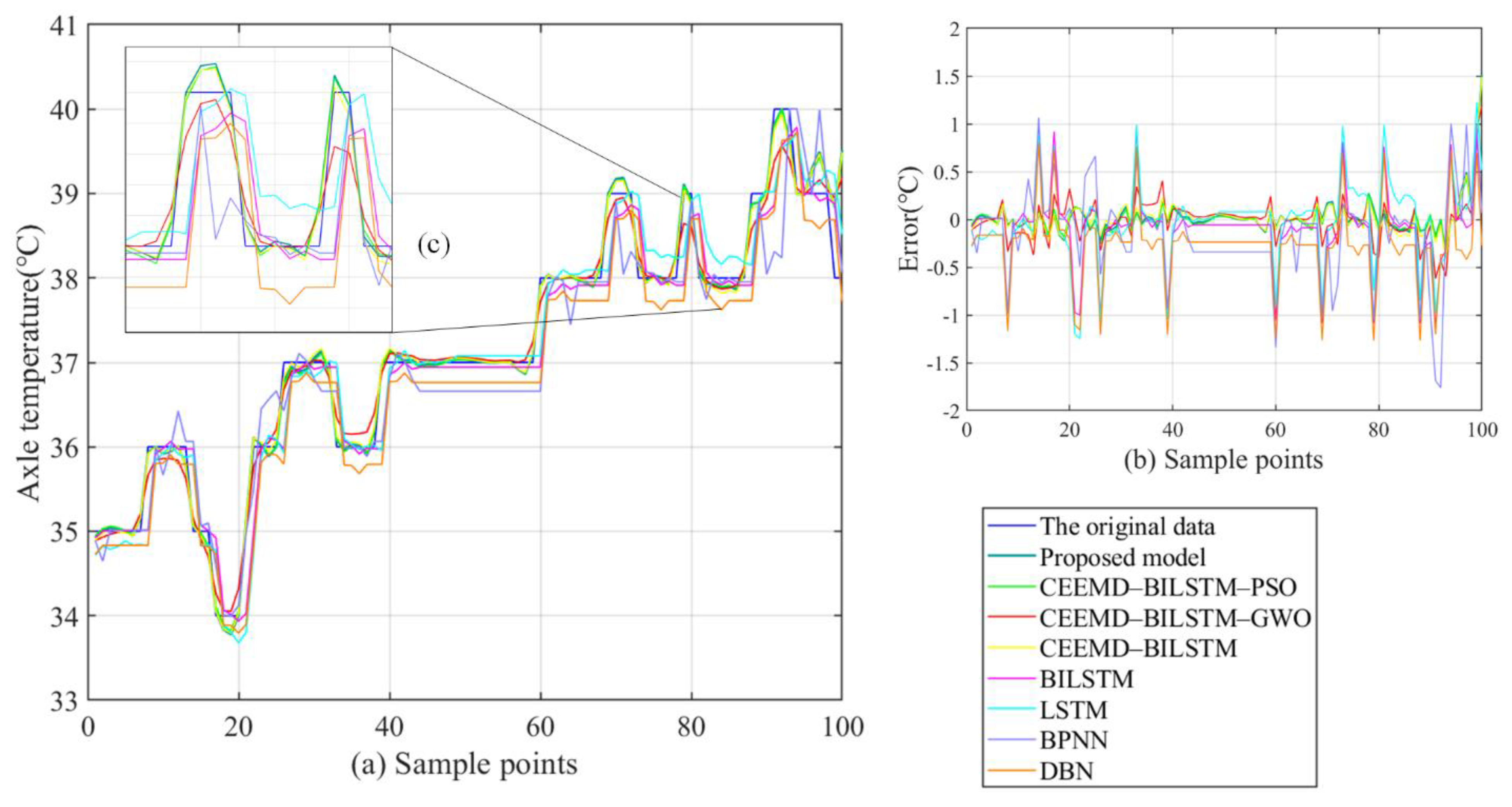
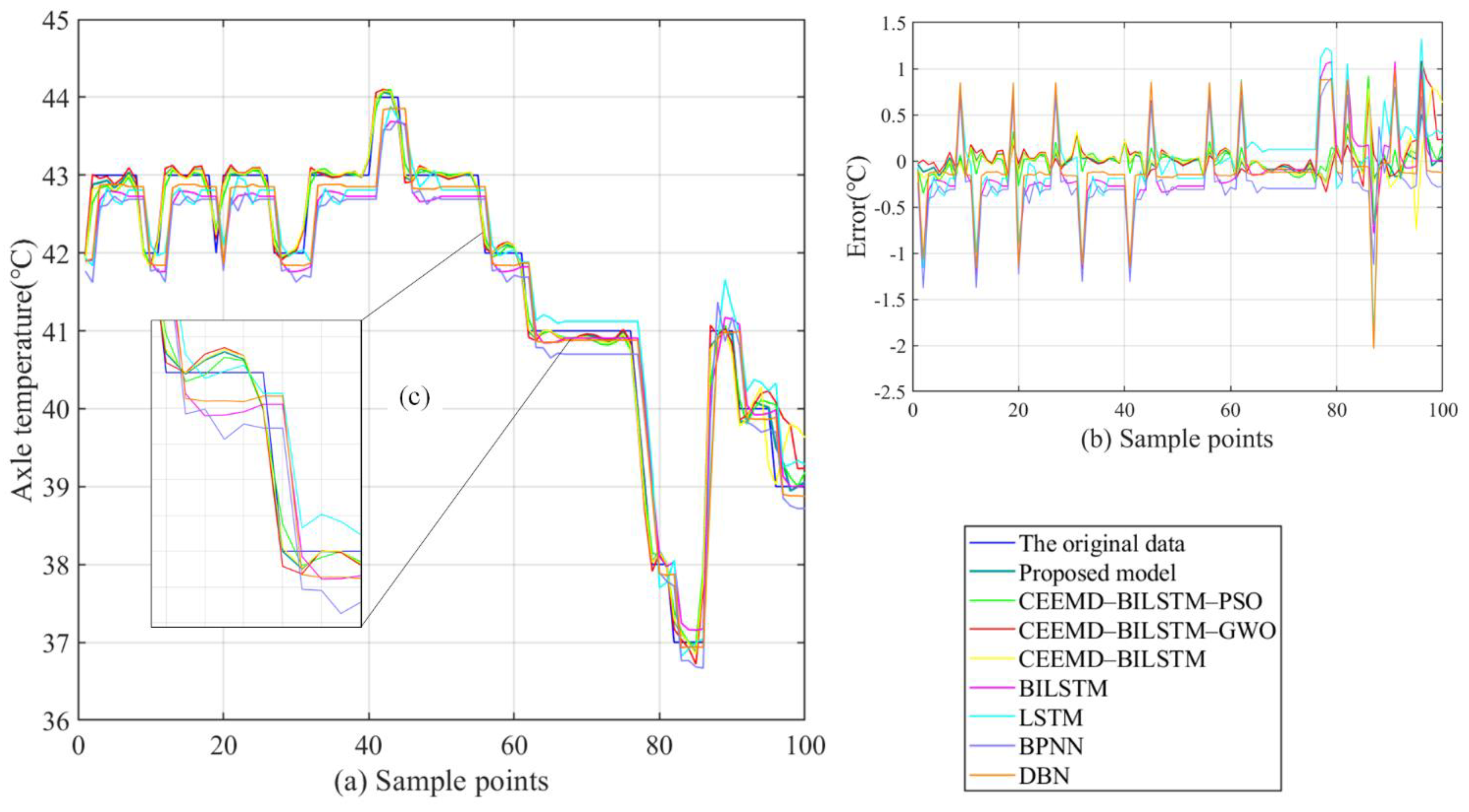
The forecasting models show satisfying accuracy and robustness for the research of temperature changes. In Figure 6, Figure 7 and Figure 8, the forecasting accuracy of the proposed CEEMD-BILSTM-PSOGSA is higher than the CEEMD-BILSTM and BILSTM model. The ensemble optimization in hybrid models could efficiently forecast the temporal trend of temperature and improve the predictive performance to more than 67%. The possible reason may be that the PSOGSA algorithm could conduct an efficient weight optimization process by the axle temperature features, which is also the first time in the data-driven approaches of the axle temperature data. The evaluation values of the CEEMD-BILSTM-PSOGSA framework is the lowest among all the models in all the datasets.

(b)

The hybrid model also outperforms the classical single predictors and regression methods, which is affected by the optimization in the prediction process from many aspects. In Figure 6, Figure 7 and Figure 8, all the hybrid models have better forecasting accuracies than the single predictors in all datasets. In addition to the deep networks’ ability to process nonstationary data, the proposed hybrid models are highly adaptable, so the decomposition methods and optimization algorithms effectively analyze and simulate the trend of nonstationary and nonlinear data, which contributed to better accuracy than the single models and the effective application of hybrid models indicates a possible research direction of time-series prediction for the early warning.

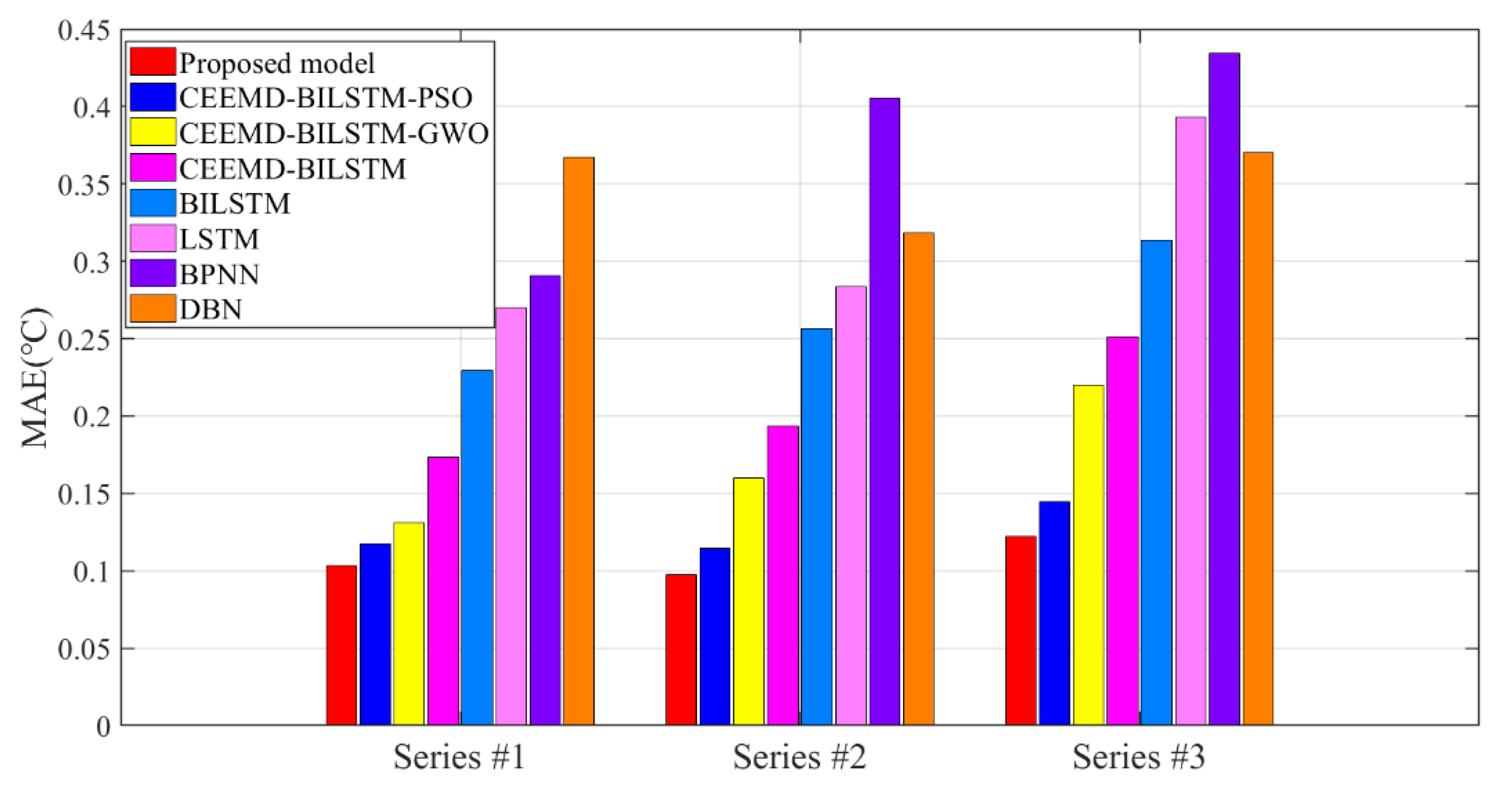
(c)

The proposed CEEMD-BILSTM-PSOGSA model obtains the best forecasting results of all data series with the evaluation indexes. The MAE can reach less than 0.1 °C and the MAPE can achieve almost 0.2%. Compared with other hybrid models, the proposed model still outperforms them from 11.9% to 47.7% in the indexes. Figure 10, Figure 11 and Figure 12 show the final forecasting results and the deviation from the original data of all the models. The predicted values of the proposed model are closer to the original data than others. Figure 9 represents the changes in the loss during the iterations of PSOGSA, PSO, and GWO. In comparison, the PSOGSA has a faster convergence speed and a lower final loss than PSO and GWO in all the datasets, which credits the excellent exploration and the research localization abilities from the combination of the PSO and GSA algorithms. Thus, the CEEMD-BILSTM-PSOGSA model integrates the superiorities of the single algorithms and has excellent application foregrounds in axle temperature forecasting.

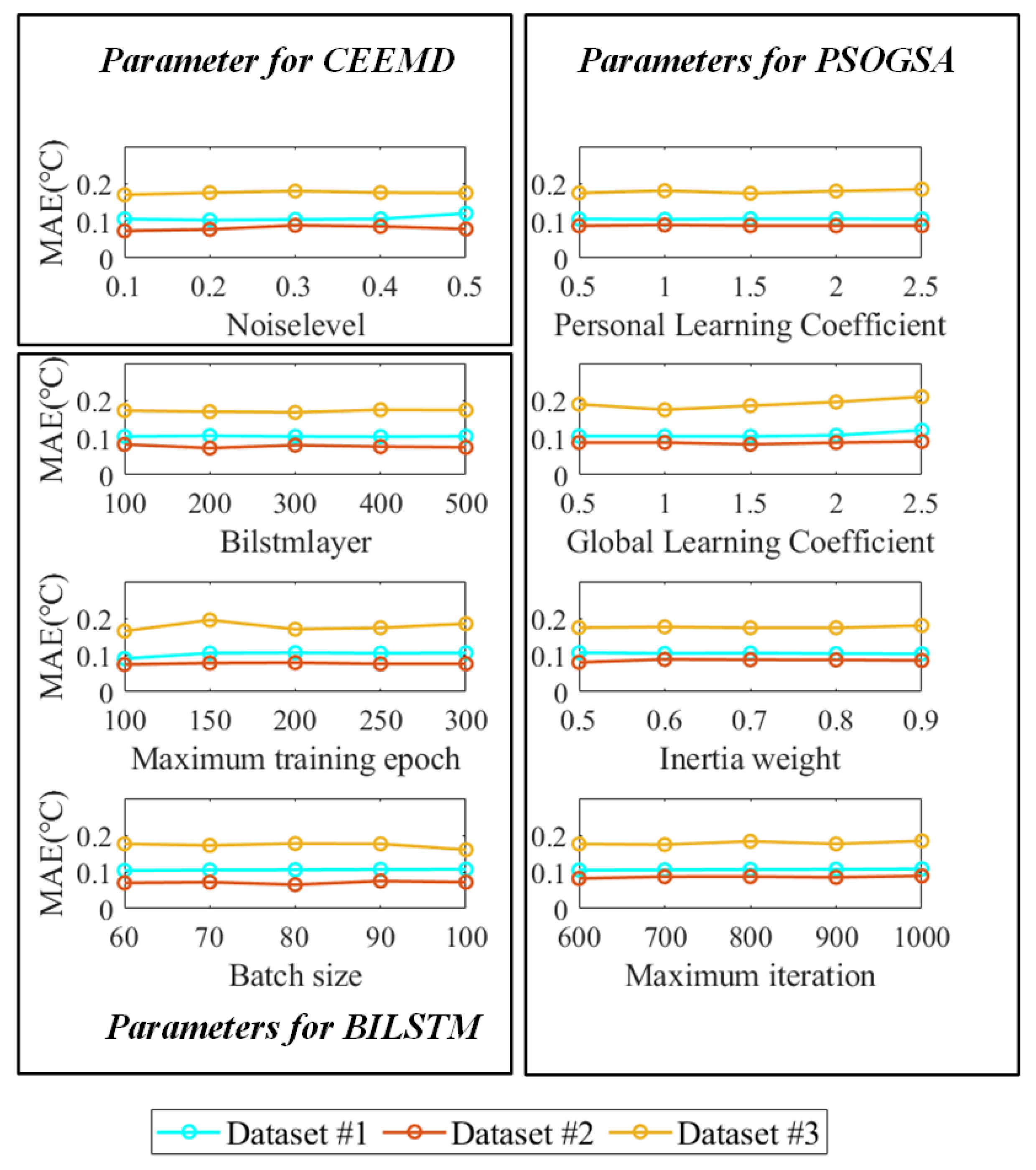
3.5. Sensitive Analysis of the Parameters and the Validation of the Model

In this paper, the sensitivity of the parameters of the proposed model is also analyzed. Each parameter will be tested by five different values. The results of the important parameters are listed in Figure 13. The MAEs stand for forecasting accuracy. It could be found that the proposed framework is generally reliable and robust to the parameters with a few fluctuations by different settings. For example, when the personal learning coefficient is 1.5, the MAEs obtain the smallest values to be regarded as the best forecasting accuracy. In the maximum iterations of PSOGSA, the changing of the parameter value has little influence on the results of the proposed model. For the short calculation time, it is rational to set the maximum iterations at 600.

The hybrid framework has been tested on three axle temperature datasets, and the results for deviation in Table 3, Table 4, Table 5, Table 6 and Table 7 are stable, which are obtained by repeated experiments without too much fluctuation. The changing trends of different temperature datasets also did not reduce the accuracy of the model results. Therefore, the reliability and robustness of the proposed model have been validated on different datasets, so it can effectively analyze the fluctuation features of axle temperature series. Therefore, it can be applied to precisely forecast the changing trends of different axle temperature datasets. The involved single predictors cannot relatively complete the information mining from the collected datasets, which leads to inaccuracy in axle temperature forecasting. Therefore, the reliability and robustness of the proposed model have been significantly improved compared with single predictors.

4. Conclusions and Future Work

In the paper, a novel axle temperature forecasting model was constructed by integrating the CEEMD method, the BILSTM neural network, and the PSOGSA optimization algorithm. In the proposed framework, the CEEMD was used to preprocess the raw irregular data into a set of sub-layers, which can facilitate the prediction of the next step. The BILSTM is applied for the prediction for each sub-layer. The PSOGSA algorithm would continue optimizing the initial value of forecasting results from each sub-layer and combine them for the final data. To study the forecasting capability of the proposed CEEMD-BILSTM-PSOGSA model, other benchmark predictors and hybrid models are listed and observed in the comparative research. From the results of the above experiments, the following conclusions can be drawn:

(a)

The predictive performance of the deep networks with bidirectional operation structure is better than regression methods and shallow neural networks. The deep structure can contribute to the analysis of the fluctuation and nonlinear features of the axle temperature datasets. Therefore, the prediction by the deep networks has an effective application in the research of axle temperature forecasting.

(b)

The proposed model proved the fact that the decomposition algorithms can efficiently raise the accuracy of the BILSTM. In the EMD series, the CEEMD showed excellent adaptive decomposition ability in the process of the axle temperature data and had a positive effect to improve the predictive ability rather than the EEMD and the EMD in all data series.

(c)

The ensemble process based on the PSOGSA optimization algorithm is significantly better for the integration of deep network sub-series and for an improvement of the prediction accuracy. Besides, the optimization levels of the proposed algorithm also outperform the PSO and GWO algorithms.

(d)

Compared with the classical predictors and other involved hybrid models, the proposed effective model combined all advantages of the components and presented a good prediction ability and adaptability in axle temperature forecasting, which offered a new approach for the prediction and early warning for the effective axle temperature research.

The proposed model can be utilized for accurate axle temperature forecasting. Therefore, it can be effectively used in locomotive early warning systems. Some research could be conducted for the further improvement of the model:

(a)

The proposed model used a univariate axle temperature framework by time series, which may be affected by the historical data. Moreover, the accuracy and reliability of the model will be in recession according to the locomotive running period. To guarantee the regular function of the model, it is necessary to update model parameters and to take the correlation by multivariate of the operating environment into consideration.

(b)

This paper aims to the short-term forecasting research of locomotive axle temperature. For the massive data generated by the locomotive during long-term operation in the future, an effective data processing platform can conduct a more comprehensive analysis of the locomotive. Within the application of the big data platform technology, the proposed hybrid model can be embedded into the distributed computing system for further application in the big data platform.

References

- Li, C.; Luo, S.; Cole, C.; Spiryagin, M. An overview: Modern techniques for railway vehicle on-board health monitoring systems. Veh. Syst. Dyn. 2017, 55, 1045–1070. [Google Scholar] [CrossRef]
- Wu, S.C.; Liu, Y.X.; Li, C.H.; Kang, G.; Liang, S.L. On the fatigue performance and residual life of intercity railway axles with inside axle boxes. Eng. Fract. Mech. 2018, 197, 176–191. [Google Scholar] [CrossRef]
- Ma, W.; Tan, S.; Hei, X.; Zhao, J.; Xie, G. A Prediction Method Based on Stepwise Regression Analysis for Train Axle Temperature. In Proceedings of the 12th International Conference on Computational Intelligence and Security, Wuxi, China, 16–19 December 2016; pp. 386–390. [Google Scholar]
- Milic, S.D.; Sreckovic, M.Z. A Stationary System of Noncontact Temperature Measurement and Hotbox Detecting. IEEE Trans. Veh. Technol. 2008, 57, 2684–2694. [Google Scholar] [CrossRef]
- Singh, P.; Huang, Y.P.; Wu, S.-I. An Intuitionistic Fuzzy Set Approach for Multi-attribute Information Classification and Decision-Making. Int. J. Fuzzy Syst. 2020, 22, 1506–1520. [Google Scholar] [CrossRef]
- Bing, C.; Shen, H.; Jie, C.; Li, L. Design of CRH axle temperature alarm based on digital potentiometer. In Proceedings of the Chinese Control Conference, Chengdu, China, 27–29 July 2016. [Google Scholar]
- Vale, C.; Bonifácio, C.; Seabra, J.; Calçada, R.; Mazzino, N.; Elisa, M.; Terribile, S.; Anguita, D.; Fumeo, E.; Saborido, C. Novel efficient technologies in Europe for axle bearing condition monitoring—The MAXBE project. Transp. Res. Procedia 2016, 14, 635–644. [Google Scholar] [CrossRef] [Green Version]
- Liu, Q. High-speed Train Axle Temperature Monitoring System Based on Switched Ethernet. Procedia Comput. Sci. 2017, 107, 70–74. [Google Scholar] [CrossRef]
- Yuan, H.; Wu, N.; Chen, X.; Wang, Y. Fault Diagnosis of Rolling Bearing Based on Shift Invariant Sparse Feature and Optimized Support Vector Machine. Machines 2021, 9, 98. [Google Scholar] [CrossRef]
- Pham, M.-T.; Kim, J.-M.; Kim, C.-H. 2D CNN-Based Multi-Output Diagnosis for Compound Bearing Faults under Variable Rotational Speeds. Machines 2021, 9, 199. [Google Scholar] [CrossRef]
- Yang, X.; Dong, H.; Man, J.; Chen, F.; Zhen, L.; Jia, L.; Qin, Y. Research on Temperature Prediction for Axles of Rail Vehicle Based on LSTM. In Proceedings of the 4th International Conference on Electrical and Information Technologies for Rail Transportation (EITRT), Singapore, 25–27 October 2019; pp. 685–696. [Google Scholar]
- Luo, C.; Yang, D.; Huang, J.; Deng, Y.D.; Long, L.; Li, Y.; Li, X.; Dai, Y.; Yang, H. LSTM-Based Temperature Prediction for Hot-Axles of Locomotives. ITM Web Conf. 2017, 12, 01013. [Google Scholar] [CrossRef] [Green Version]
- Yan, G.; Yu, C.; Bai, Y. Wind Turbine Bearing Temperature Forecasting Using a New Data-Driven Ensemble Approach. Machines 2021, 9, 248. [Google Scholar] [CrossRef]
- Mi, X.; Zhao, S. Wind speed prediction based on singular spectrum analysis and neural network structural learning. Energy Convers. Manag. 2020, 216, 112956. [Google Scholar] [CrossRef]
- Gou, H.; Ning, Y. Forecasting Model of Photovoltaic Power Based on KPCA-MCS-DCNN. Comput. Model. Eng. Sci. 2021, 128, 803–822. [Google Scholar] [CrossRef]
- Wang, H.; Li, G.; Wang, G.; Peng, J.; Jiang, H.; Liu, Y. Deep learning based ensemble approach for probabilistic wind power forecasting. Appl. Energy 2017, 188, 56–70. [Google Scholar] [CrossRef]
- Zhang, X.; Zhang, Q. Short-Term Traffic Flow Prediction Based on LSTM-XGBoost Combination Model. Comput. Model. Eng. Sci. 2020, 125, 95–109. [Google Scholar] [CrossRef]
- Dong, S.; Yu, C.; Yan, G.; Zhu, J.; Hu, H. A Novel Ensemble Reinforcement Learning Gated Recursive Network for Traffic Speed Forecasting. In Proceedings of the 2021 Workshop on Algorithm and Big Data, Fuzhou, China, 12–14 March 2021; pp. 55–60. [Google Scholar]
- Liu, X.; Qin, M.; He, Y.; Mi, X.; Yu, C. A new multi-data-driven spatiotemporal PM2.5 forecasting model based on an ensemble graph reinforcement learning convolutional network. Atmos. Pollut. Res. 2021, 12, 101197. [Google Scholar] [CrossRef]
- Mashaly, A.F.; Alazba, A.A. MLP and MLR models for instantaneous thermal efficiency prediction of solar still under hyper-arid environment. Comput. Electron. Agric. 2016, 122, 146–155. [Google Scholar] [CrossRef]
- Lee, H.; Han, S.-Y.; Park, K.; Lee, H.; Kwon, T. Real-Time Hybrid Deep Learning-Based Train Running Safety Prediction Framework of Railway Vehicle. Machines 2021, 9, 130. [Google Scholar] [CrossRef]
- Hong, S.; Zhou, Z.; Zio, E.; Wang, W. An adaptive method for health trend prediction of rotating bearings. Digit. Signal Process. 2014, 35, 117–123. [Google Scholar] [CrossRef]
- Wang, H.; Liu, L.; Dong, S.; Qian, Z.; Wei, H. A novel work zone short-term vehicle-type specific traffic speed prediction model through the hybrid EMD–ARIMA framework. Transp. B Transp. Dyn. 2016, 4, 159–186. [Google Scholar] [CrossRef]
- Bai, Y.; Zeng, B.; Li, C.; Zhang, J. An ensemble long short-term memory neural network for hourly PM2.5 concentration forecasting. Chemosphere 2019, 222, 286–294. [Google Scholar] [CrossRef]
- Chang, Y.; Fang, H.; Zhang, Y. A new hybrid method for the prediction of the remaining useful life of a lithium-ion battery. Appl. Energy 2017, 206, 1564–1578. [Google Scholar] [CrossRef]
- Hao, W.; Liu, F. Axle Temperature Monitoring and Neural Network Prediction Analysis for High-Speed Train under Operation. Symmetry 2020, 12, 1662. [Google Scholar] [CrossRef]
- Zhang, B.; Zhang, H.; Zhao, G.; Lian, J. Constructing a PM2.5 concentration prediction model by combining auto-encoder with Bi-LSTM neural networks. Environ. Model. Softw. 2020, 124, 104600. [Google Scholar] [CrossRef]
- Kouchami-Sardoo, I.; Shirani, H.; Esfandiarpour-Boroujeni, I.; Besalatpour, A.A.; Hajabbasi, M.A. Prediction of soil wind erodibility using a hybrid Genetic algorithm—Artificial neural network method. CATENA 2020, 187, 104315. [Google Scholar] [CrossRef]
- Xing, Y.; Yue, J.; Chen, C.; Xiang, Y.; Shi, M. A Deep Belief Network Combined with Modified Grey Wolf Optimization Algorithm for PM2.5 Concentration Prediction. Appl. Sci. 2019, 9, 3765. [Google Scholar] [CrossRef] [Green Version]
- Singh, P. A novel hybrid time series forecasting model based on neutrosophic-PSO approach. Int. J. Mach. Learn. Cybern. 2020, 11, 1643–1658. [Google Scholar] [CrossRef]
- Zhang, Y.; Cui, N.; Feng, Y.; Gong, D.; Hu, X. Comparison of BP, PSO-BP and statistical models for predicting daily global solar radiation in arid Northwest China. Comput. Electron. Agric. 2019, 164, 104905. [Google Scholar] [CrossRef]
- Zhu, S.; Yang, L.; Wang, W.; Liu, X.; Lu, M.; Shen, X. Optimal-combined model for air quality index forecasting: 5 cities in North China. Environ. Pollut. 2018, 243, 842–850. [Google Scholar] [CrossRef]
- Tan, S.; Ma, W.; Hei, X.; Xie, G.; Chen, X.; Zhang, J. High Speed Train Axle Temperature Prediction Based on Support Vector Regression. In Proceedings of the 2019 14th IEEE Conference on Industrial Electronics and Applications (ICIEA), Xi’an, China, 19–21 June 2019; pp. 2223–2227. [Google Scholar]
- Yildirim, Ö. A novel wavelet sequence based on deep bidirectional LSTM network model for ECG signal classification. Comput. Biol. Med. 2018, 96, 189–202. [Google Scholar] [CrossRef]
- Yeh, J.R.; Shieh, J.S.; Huang, N.E. Complementary Ensemble Empirical Mode Decomposition: A Novel Noise Enhanced Data Analysis Method. Adv. Adapt. Data Anal. 2010, 2, 135–156. [Google Scholar] [CrossRef]
- Huang, N.E.; Shen, Z.; Long, S.R.; Wu, M.C.; Shih, H.H.; Zheng, Q.; Yen, N.C.; Tung, C.C.; Liu, H.H. The empirical mode decomposition and the Hilbert spectrum for nonlinear and non-stationary time series analysis. Proc. Math. Phys. Eng. Sci. 1998, 454, 903–995. [Google Scholar] [CrossRef]
- Wu, Z.; Huang, N.E. Ensemble Empirical Mode Decomposition: A Noise-Assisted Data Analysis Method. Adv. Adapt. Data Anal. 2009, 1, 1–41. [Google Scholar] [CrossRef]
- Xue, X.; Zhou, J.; Xu, Y.; Zhu, W.; Li, C. An adaptively fast ensemble empirical mode decomposition method and its applications to rolling element bearing fault diagnosis. Mech. Syst. Signal Process. 2015, 62–63, 444–459. [Google Scholar] [CrossRef]
- Zhu, S.; Lian, X.; Wei, L.; Che, J.; Shen, X.; Yang, L.; Qiu, X.; Liu, X.; Gao, W.; Ren, X.; et al. PM2.5 forecasting using SVR with PSOGSA algorithm based on CEEMD, GRNN and GCA considering meteorological factors. Atmos. Environ. 2018, 183, 20–32. [Google Scholar] [CrossRef]
- Hochreiter, S.; Schmidhuber, J. Long Short-term Memory. Neural Comput. 1997, 9, 1735–1780. [Google Scholar] [CrossRef]
- Wu, Y.; Yuan, M.; Dong, S.; Lin, L.; Liu, Y. Remaining useful life estimation of engineered systems using vanilla LSTM neural networks. Neurocomputing 2018, 275, 167–179. [Google Scholar] [CrossRef]
- Hou, M.; Pi, D.; Li, B. Similarity-based deep learning approach for remaining useful life prediction. Measurement 2020, 159, 107788. [Google Scholar] [CrossRef]
- Yildirim, O.; Baloglu, U.B.; Tan, R.-S.; Ciaccio, E.J.; Acharya, U.R. A new approach for arrhythmia classification using deep coded features and LSTM networks. Comput. Methods Programs Biomed. 2019, 176, 121–133. [Google Scholar] [CrossRef]
- Cheng, H.; Ding, X.; Zhou, W.; Ding, R. A hybrid electricity price forecasting model with Bayesian optimization for German energy exchange. Int. J. Electr. Power Energy Syst. 2019, 110, 653–666. [Google Scholar] [CrossRef]
- Schuster, M.; Paliwal, K.K. Bidirectional recurrent neural networks. IEEE Trans. Signal Process. 1997, 45, 2673–2681. [Google Scholar] [CrossRef] [Green Version]
- Kennedy, J.; Eberhart, R. Particle swarm optimization. In Proceedings of the ICNN’95-International Conference on Neural Networks, Perth, Australia, 27 November–1 December 1995; pp. 1942–1948. [Google Scholar]
- Huang, M.-L.; Chou, Y.-C. Combining a gravitational search algorithm, particle swarm optimization, and fuzzy rules to improve the classification performance of a feed-forward neural network. Comput. Methods Programs Biomed. 2019, 180, 105016. [Google Scholar] [CrossRef] [PubMed]
- Duman, S.; Yorukeren, N.; Altas, I.H. A novel modified hybrid PSOGSA based on fuzzy logic for non-convex economic dispatch problem with valve-point effect. Int. J. Electr. Power Energy Syst. 2015, 64, 121–135. [Google Scholar] [CrossRef]
- Rashedi, E.; Nezamabadi-pour, H.; Saryazdi, S. GSA: A Gravitational Search Algorithm. Inf. Sci. 2009, 179, 2232–2248. [Google Scholar] [CrossRef]
- Mirjalili, S.; Hashim, S.Z.M. A new hybrid PSOGSA algorithm for function optimization. In Proceedings of the 2010 International Conference on Computer and Information Application, Tianjin, China, 3–5 December 2010; pp. 374–377. [Google Scholar]
- Bounar, N.; Labdai, S.; Boulkroune, A. PSO–GSA based fuzzy sliding mode controller for DFIG-based wind turbine. ISA Trans. 2019, 85, 177–188. [Google Scholar] [CrossRef]
- Qu, Z.; Zhang, K.; Mao, W.; Wang, J.; Liu, C.; Zhang, W. Research and application of ensemble forecasting based on a novel multi-objective optimization algorithm for wind-speed forecasting. Energy Convers. Manag. 2017, 154, 440–454. [Google Scholar] [CrossRef]
- Kong, W.; Wang, B. Combining Trend-Based Loss with Neural Network for Air Quality Forecasting in Internet of Things. Comput. Model. Eng. Sci. 2020, 125, 849–863. [Google Scholar] [CrossRef]