Neural Network-Based Automated Assessment of Fatigue Damage in Mechanical Structures

Abstract

This paper proposes a methodology for automated assessment of fatigue damage, which has been tested and validated with polycrystalline-alloy (Aℓ7075-T6) specimens on an experimental apparatus. Based on an ensemble of time series of ultrasonic test (UT) data, the proposed procedure is found to be capable of detecting fatigue-damage (at an early stage) in mechanical structures, which is followed by online evaluation of the associated risk. The underlying concept is built upon two neural network (NN)-based models, where the first NN model identifies the feature of the UT data belonging to one of the two classes: undamaged structure and damaged structure, and the second NN model further classifies an identified damaged structure into three classes: low-risk, medium-risk, and high-risk. The input information to the second NN model is the crack tip opening displacement (CTOD), which is computed by the first NN model via linear regression from an ensemble of optical data, acquired from the experiments. Both NN models have been trained by using scaled conjugate gradient algorithms. The results show that the first NN model classifies the energy of UT signals with (up to) 98.5% accuracy, and that the accuracy of the second NN model is 94.6%.

1. Introduction

Structural integrity of large-scale systems (e.g, aircraft, large-scale transport vehicles, and power plants) deteriorates over time due to damage in their mechanical components. According to Farrar and Wonden [1], the damage is the cumulative effect of changes that are initiated in a system and potentially degrades the system reliability; these phenomena may lead to both anticipated and unanticipated failures unless appropriate timely actions are taken. Damage in mechanical structures may evolve either at a micro-scale level from inherent local defects (e.g., voids and inclusions) in materials, or at a macro-scale level from global defects (e.g., corrosion and existing cracks). The fatigue damage, which belongs to a special class of structural damage, is caused by fluctuating stresses that can be well below the respective yield points. It is well known [2,3,4] that ∼90% of the structural failures occur due to fatigue damage. In general, failures due to fatigue damage evolve through the following three stages.

• Defect generation: Defects may exist in the structural materials from which the machinery parts are manufactured, or defects may occur during the manufacturing process itself.
• Damage evolution: Fatigue damage in the structures of machinery components is an evolutionary process during the course of its operation.
• Crack propagation: As the damage in machinery components evolves, their cumulative effects may give rise to cracks that could propagate and directly affect the machinery operation, possibly leading to a complete failure and shutdown.

This paper focuses on assessment of the evolving fatigue damage in machinery structures, which plays a critical role in planning and management of machinery operation, via detection and characterization of the damage. Furthermore, the risk of health degradation of machinery components is evaluated from the assessed damage along with the estimation of a time schedule for (possibly condition-based) maintenance. Thus, damage assessment is considered to be one of the fundamental tasks that are directly related to the safety of both plant operating personnel and equipment. In general, the task of damage assessment is applicable to a variety of industrial equipment (e.g., boilers, turbines, and pumps), transport vehicles (e.g., vehicles, ships, and airplanes), and civil engineering infrastructures (e.g, buildings and bridges) [5,6,7].

Identification of occurrence, location, and severity of the damage in mechanical structures is considered to be one of the difficult tasks in damage assessment. For example, structural health monitoring (SHM) is used widely in civil infrastructures such as bridges to identify and evaluate the damage, evolving over time. Another example is condition monitoring (CM) that is used in rotating machinery for a similar purpose as SHM, but the impact of the environment on CM is limited as compared to that of SHM [8,9,10,11].

In many industries, the expertise of (human) inspectors is essential for damage assessment (e.g., making a decision on when a critical structure should be taken out of service for maintenance), which is expensive and error-prone. Therefore, various automated methods of fatigue-damage assessment have emerged for the dual purpose of damage detection and assessment (i.e., quantification). To this end, the work reported in this paper develops an automated method of fatigue-damage assessment to assist the maintenance team in making timely and feasible decisions.

Two models have been developed on the principle of neural networks, hereafter abbreviated as NN. These NN-based models, reported in the paper, have been developed, tested, and validated on laboratory-scale experimental apparatuses, where the most effective failure factor is the applied fatigue loads on the test specimens; and other less significant factors (e.g., environmental effects) are not addressed in this paper [12,13,14]. The first model is built upon NN analysis of an ensemble of ultrasonic testing (UT) signals, which is used to identify the onset of fatigue damage in the test specimens. The second NN model is developed based on optical images from a confocal microscope and a digital microscope, which measure the surface topography and the crack tip opening displacement (CTOD) to define three levels (i.e., low, medium, and high) of damage risk. The data base for CTOD is augmented as a function of the measurements of crack length from a digital microscope. In summary, the reported work focuses on real-time assessment of fatigue damage and the associated risk analysis for structural materials, made of polycrystalline alloys.

Contributions of the paper: The major contributions of this paper are delineated below.

• Extraction of relevant features: The extracted features are used for detection of structural damage and classification of damage risk.
• Development of an analytical model relating the crack length with the CTOD: The information on the estimated CTOD data (which are derived from the measured data of crack length) is used as input data for NN models.
• Construction of a neural-network-based pattern classifier: The first stage of the neural network classifies the features of ultrasonic data into the categories of undamaged structure and damaged structure in the first stage of the proposed method, while the second stage classifies the information on CTOD into low-risk, medium-risk, and high-risk.

Organization of the paper: The paper is organized into five sections. Section 2 describes the laboratory apparatus that serves as the data generator for validation of the reported method of fatigue-damage assessment. Section 3 illustrates the methodology adopted in this paper, including an overview of linear regression and neural networks; this section consists of the following three subsections: the concept of curve fitting by linear regression; an overview of neural networks; and online damage assessment in mechanical structures. Section 4 discusses the results generated from the proposed method. Section 5 summarizes and concludes the paper along with recommendations for future research.

2. Description of the Experimental Apparatus

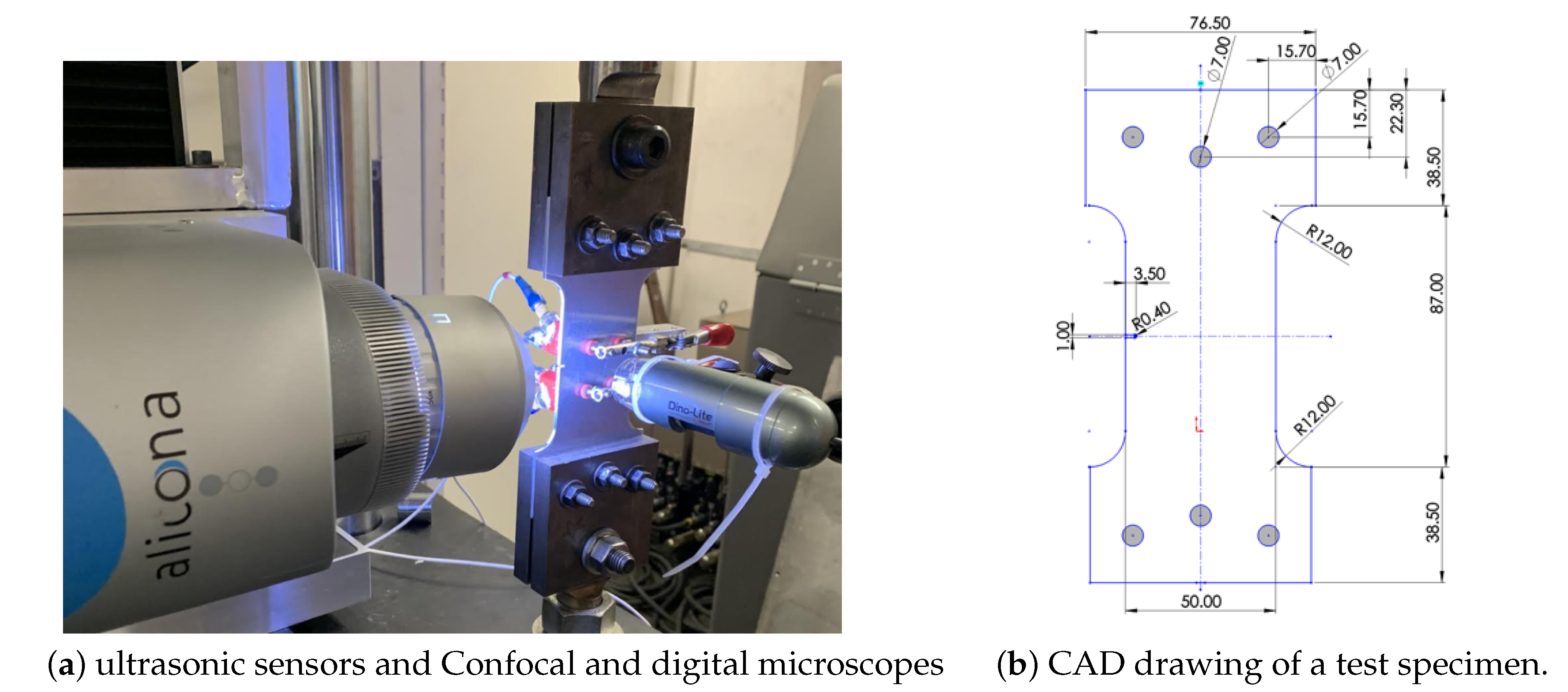
This section describes the experimental apparatus, as shown in Figure 1a, which is built upon a computer-instrumented and computer-controlled fatigue testing machine (Manufacturer: MTS Systems Corporation, Berlin, NJ, USA), equipped with ultrasonic testing probes (Manufacturer: Olympus, Tokyo, Japan), a confocal microscope (Manufacturer: Alicona Imaging GmbH | Dr.-Auner-Strasse 21a | 8074 Raaba/Graz, Austria), and a digital microscope (Manufacturer: QUESTAR^®, New Hope, Pennsylvania, USA). The main objective here is to acquire ensembles of fatigue test data for evaluation of the damage state of the structure under consideration (e.g., test specimens in the experiments). In general, under medium-cycle to high-cycle fatigue loading of (ductile-alloy) machinery structures, a good part of the service life is consumed before reaching the crack onset stage. Therefore, the knowledge on the onset of fatigue cracks is necessary to reduce the probability of unanticipated failures as well as to maintain the machinery performance, which enhances both reliability and availability of machinery operation at a mitigated maintenance cost.

Results from 18 typical experiments have been reported to help formulating a strategy of structural health management in terms of the fatigue-damage properties of polycrystalline alloys. Figure 1b shows the CAD drawing of a notched test specimen (made of Aℓ7075-T6 alloy), where each specimen is 3 mm thick with a 50 mm wide gauge section and the flanges with three holes on both ends are 76.5 mm wide to fix the specimens on the test apparatus by using custom-made grips.

Table 1. The mechanical properties of Aℓ7075-T6 alloy.

Mechanical Properties	The Value
Ultimate Tensile Strength (MPa)	572
Tensile Yield Strength (MPa)	503
Modulus of Elasticity (GPa)	71.7
Fatigue Strength (MPa)	159

presents the mechanical properties of Aℓ7075-T6 alloy.

2.1. Ultrasonic Testing

In the ultrasonic testing (UT) probes (see Figure 1), high frequency acoustic pulses (i.e., 15 MHz ultrasonic waves) are injected into each specimen by a piezo-electric transducer, called the transmitter, and are received by another piezo-electric transducer called the receiver, which is located on the other side of the transmitter. The strength of the signal is measured after it has propagated through the material. The strength of the signal at the receiver is influenced by the material features (e.g., grain boundaries, voids, and inclusions) that exist on the path of the propagated signals. While the effects of the pre-existing flaws such as voids, inclusions, or grain boundaries on the signal strength are assumed to be very gradually evolving and stable over the crack onset stage of the structure, the strength of the signal decreases dramatically once the crack propagation starts through the material because significant parts of the signals are reflected back and thus do not reach the receiver.

2.2. Optical Metrology Device

The optical metrology device (Infinite-Focus Alicona) (see Figure 1) provides 3D surface images. In the Focus-Variation system of Alicona, the topographical (colored) information is created from variations in the focus, where the small depth of the focus in an optical system is combined with vertical scanning. The vertical resolution of the Infinite-Focus system can be as low as 20 nm. The size of the generated image using Alicona is 0.4 mm by 0.4 mm, and each image has 4,161,600 pixels. Thus, the Alicona optical metrology device has the ability to detect very small cracks that are significantly less than 0.25 mm; these crack lengths are considered in this paper to belong to the crack onset regime. In the experiments, Alicona images have been taken (approximately) synchronously with ultrasonic testing (UT) data in order to provide a ground truth for the results of analysis from UT signals. Since the Alicona metrology also provides information on surface topography, they have been used to measure both the surface average roughness ($S_{\alpha }$, the arithmetical mean height of a surface) and crack tip opening displacement (CTOD) [15,16].

2.3. Digital Microscope

Measurements from the Quester digital microscope (QDM) (see Figure 1), were taken synchronously with the measurements of average roughness ($S_{\alpha }$) and crack tip opening displacement (CTOD) to provide the corresponding crack length $\alpha$. The image resolution of the QDM is 640 × 480 pixels and the images are taken with 10-200X variable magnification.

3. Methodology of Damage Analysis

This section briefly introduces the methodologies, adopted in this paper for analysis of the experimental data (see Section 2), including overviews of linear regression, neural networks, and online damage assessment.

3.1. Curve Fitting by Linear Regression

Curve fitting by linear least squares is a method of identifying the model that delivers the best fit to the particular curves of the available (e.g., experimental) data set, where the error of the model is the least in some sense. The least-square method is the simplest and most widely used statistical technique for minimizing the error of the model (i.e., the summed square of residuals). The residuals ($r_i$) are defined as the differences between the observed responses ($y_i$) and estimated results, (${\widehat{y}}_i$) [17,18].

$$r_i=y_i-{\widehat{y}}_{i}fori=1,2,...n.$$

(1)

The residual vector r is the length of the n-array of $r_i$ values. The summed square of residuals is estimated as follows:

$$S=\sum _{i=1}^n{r}_i^2=\sum _{i=1}^n{(y_i-{\widehat{y}}_i)}^2$$

(2)

For linear least squares, the summed square of residuals in Equation (2) is estimated as:

$$S=\sum _{i=1}^n{(y_i-(a+b{x}_i))}^2$$

(3)

where the parameters a and b need to be estimated, such that S is minimized. Hence, S in Equation (3) is differentiated with respect to each parameter $\mathit{a}$ and $\mathit{b}$, and the results must be identically equal zero at an extremal point.

$$\frac{\mathrm{\partial }\mathit{S}}{\mathrm{\partial }\mathit{a}}=-\mathbf{2}\sum _{\mathit{i}=\mathbf{1}}^{\mathit{n}}({\mathit{y}}_{\mathit{i}}-(\mathit{a}+{\mathit{bx}}_{\mathit{i}}))=\mathbf{0}$$

(4)

$$\frac{\mathrm{\partial }\mathit{S}}{\mathrm{\partial }\mathit{b}}=-\mathbf{2}\sum _{\mathbf{i}=\mathbf{1}}^{\mathit{n}}{\mathit{x}}_{\mathit{i}}({\mathit{y}}_{\mathit{i}}-(\mathit{a}+{\mathit{bx}}_{\mathit{i}}))=\mathbf{0}$$

(5)

The parameters $\mathit{a}$ and $\mathit{b}$ are obtained by simultaneously solving Equations (6) and (7) as:

$$\mathit{b}=\frac{\mathit{n}\sum {\mathit{x}}_{\mathit{i}}{\mathit{y}}_{\mathit{i}}-\sum {\mathit{x}}_{\mathit{i}}\sum {\mathit{y}}_{\mathit{i}}}{\mathit{n}\sum {\mathit{x}}_{\mathit{i}}^{\mathbf{2}}-{(\sum {\mathit{x}}_{\mathit{i}})}^{\mathbf{2}}}$$

(6)

$$\mathit{a}=\frac{\mathbf{1}}{\mathit{n}}(\sum {\mathit{y}}_{\mathit{i}}-\mathit{b}\sum {\mathit{x}}_{\mathit{i}})$$

(7)

3.2. Neural Network

Neural network (NN) is a computational method that attempts to mimic the logic of a human brain. The neural network, in its simplest form, is composed of a set of nodes and a set of connections that link the neurons layerwise. Hence, an NN tends to imitate the most vital mechanism of the brain, which is the neural association. In essence, an NN works by building connections between nodes, and different types of connections create different types of NN. The feed-forward neural network is considered to be one of the most common types of NN.

3.2.1. Feed-Forward Neural Network

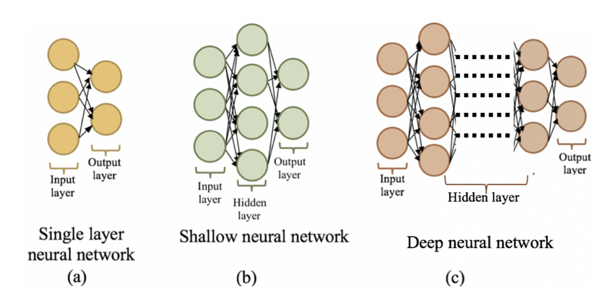
The sequence of processes in a feed-forward neural network (FFNN) is simple and unidirectional, where the sequence starts from input nodes and ends at the output nodes. While the complexity of FFNN may vary from a simple architecture to more complex architectures, the simplest architecture of FFNN is a single-layer neural network as seen in Figure 2a that is composed of an input layer (which is not counted as an NN layer) and an output layer. The second type of neural network architecture is a Shallow or Vanilla multi-layer neural network as seen in Figure 2b that consists of an input layer, one (or a few) hidden layer(s), and an output layer. If there are several hidden layers, the neural network architecture is called a deep neural network [19] as seen in Figure 2c. The rationale for defining the architecture in terms of hidden layers is that these layers are not accessible from outside of the neural network.

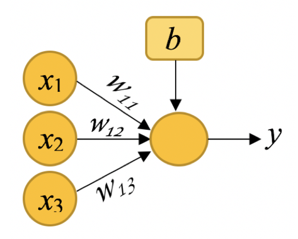
Figure 3 illustrates the basic operation of an artificial neuron, where the input data (${\mathit{x}}_{\mathbf{1}}$, ${\mathit{x}}_{\mathbf{2}}$, ${\mathit{x}}_{\mathbf{3}}$) are multiplied by weights (${\mathit{w}}_{\mathbf{11}}$, ${\mathit{w}}_{\mathbf{12}}$, ${\mathit{w}}_{\mathbf{13}}$), respectively, and added with a bias b before leaving the node. By transforming the above result by a (nonlinear) activation function $\mathit{\varphi }$, then the output $\mathit{y}$ is:

$$\begin{array}{c}\hfill \mathit{a}=\mathit{w}\ast \mathit{x}+\mathit{b}={\mathit{w}}_{\mathbf{11}}{\mathit{x}}_{\mathbf{1}}+{\mathit{w}}_{\mathbf{12}}{\mathit{x}}_{\mathbf{2}}+{\mathit{w}}_{\mathbf{3}}{\mathit{x}}_{\mathbf{13}}+\mathit{b}\end{array}$$

(8)

$$\mathit{y}=\mathit{\varphi }\left(\mathit{a}\right)=\mathit{\varphi }(\mathit{wx}+\mathit{b})$$

(9)

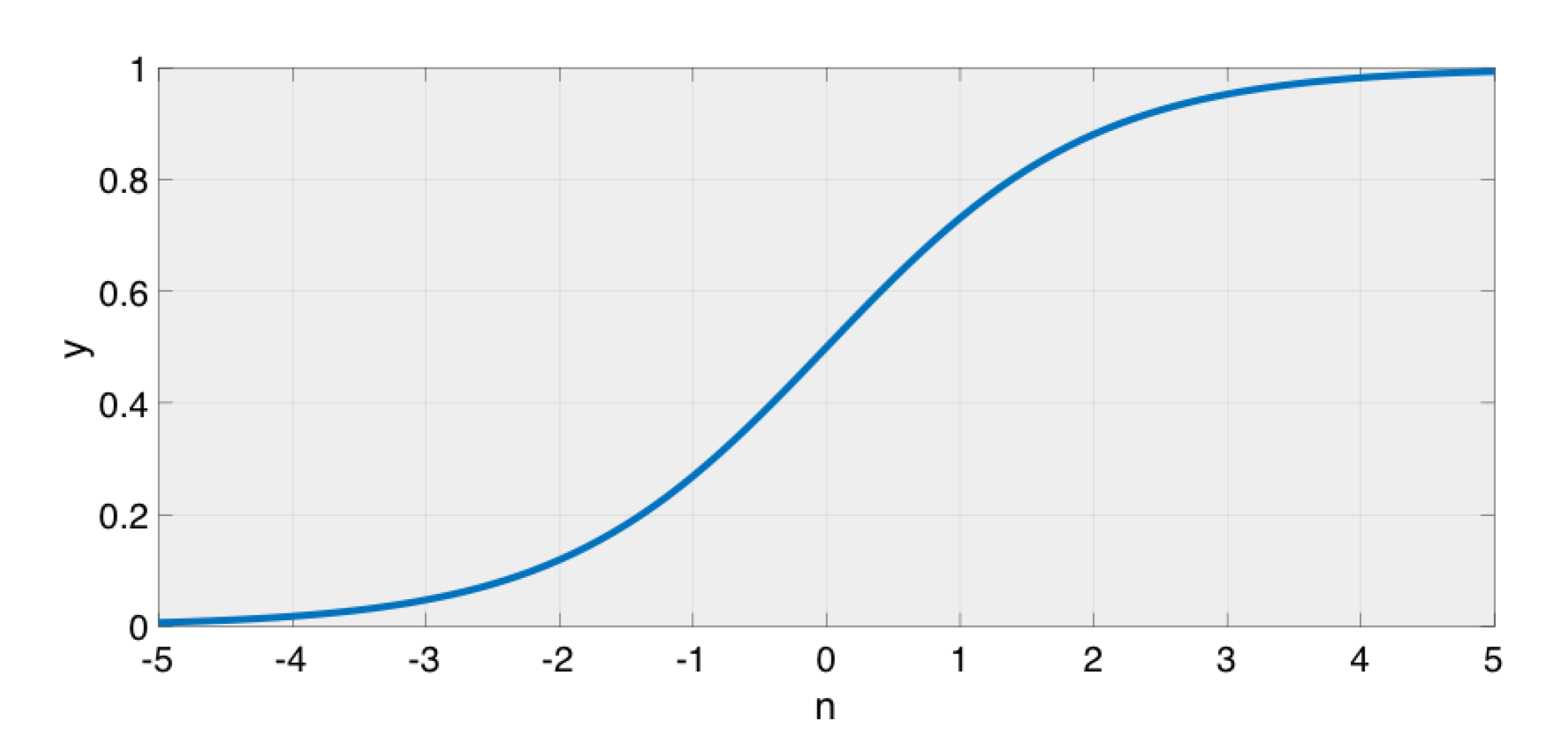
One of the popular activation functions that are used in neural networks is the (smooth and nonlinear) sigmoid function that generates an analogue output that is limited between 0 and 1, as shown in Figure 4. The sigmoid function is described by:

$$\mathit{y}=\frac{\mathbf{1}}{\mathbf{1}+\mathit{e}{}^{\mathit{a}}}$$

(10)

Another function that is used in neural networks is the softmax function, which is usually applied at the last layer in the NN architecture. This layer is used to convert the output of the hidden layer into normalized class probabilities. The softmax function is defined as:

$${\mathit{f}}_{\mathit{j}}\left(\mathit{z}\right)=\frac{{\mathit{e}}^{{\mathit{z}}_{\mathit{j}}}}{{\sum }_{\mathit{k}}{\mathit{e}}^{{\mathit{z}}_{\mathit{k}}}}$$

(11)

In essence, the softmax layer delivers the probabilities of each output class, where it takes in a vector with real values and produces a vector with elements between zero and one that sum to one.

The information in neural networks is stored in terms of weights. These weights are adjusted during the training of the neural network based on the error that is the difference between the output of the neural networks and the correct output [20,21,22,23].

3.2.2. Back Propagation

In the training/learning phase, the connection weights (${\mathit{w}}_{\mathit{ij}}$) are adjusted to improve the performance of the NN model. From the perspectives of NN, an epoch refers to one cycle of the training/learning phase. At each epoch, a set of input data are passed through the NN architecture producing outputs, and these outputs are compared with the target set of the output. Based on the computed error, the back-propagation algorithm is applied, where the measured error is passed in the reverse direction of the architecture, from the output layer to the input layer, to re-adjusted weights. This procedure is repeated continuously for the next epochs until the desired error is admissible. The mean squared error of the NN is expressed as:

$${\mathit{J}}_{\mathit{NN}}=\frac{\mathbf{1}}{\mathit{N}}\sum _{\mathit{t}=\mathbf{1}}^{\mathit{N}}\sum _{\mathit{e}=\mathbf{1}}^{\mathit{O}}{({\mathit{T}}_{{}_{\mathit{NN}}}(\mathit{t},\mathit{e})-{\mathit{y}}_{{}_{\mathit{NN}}}(\mathit{t},\mathit{e}))}^{\mathbf{2}}$$

(12)

where

• N: Number of trained data (input, output).
• e: Index identifying the output.
• t: Index identifying training data.
• O: Number of the NN outputs.
• T: The NN target values.

3.2.3. Gradient Descent (GD)

The gradient descent method (also called steepest descent) is used to adjust the weights in the direction of the performance function that declines most rapidly (e.g., the most negative of the possible gradients). Equation (13) presents the adjustment of one of the network weights by using the GD algorithm:

$${\mathit{w}}_{\mathit{n}+\mathbf{1}}={\mathit{w}}_{\mathit{n}}-\mathbf{2}\mathit{\alpha }{\mathit{J}}_{\mathit{n}}{\mathit{E}}_{\mathit{n}}$$

(13)

where

• n: Number of iteration.
• J: Jacobian matrix of ${\mathit{J}}_{{}_{\mathit{ANN}}}$.
• E: The computed error between ANN outputs and the target.

Although the GD algorithm is a well-known optimization method, it has the following four main disadvantages [24,25]:

• The learning rate is low.
• The direction is not perfectly scaled (i.e., convergence depends on the scale of the problem).
• The local minimal point could be missed.
• The results are sensitive to exogenous noise.

3.2.4. Conjugate Gradient

One of the methods that are established to improve the performance of the above GD algorithm belongs to the class of conjugate gradient (CG) algorithms. The CG algorithms are executed by searching in the steepest descent direction on the first iteration. Subsequently, a line search is implemented to find the optimal point to reach along the current search direction. Then, the next search direction is established such that it is conjugate to prior search directions. Generally, determining the new search direction requires a trade-off between the new steepest descent direction and the previous search direction as explained below:

$${\mathit{p}}_{\mathbf{0}}=-{\mathit{g}}_{\mathbf{0}},\mathit{where}\mathit{g}={\mathit{J}}^{\mathit{T}}\mathit{E}$$

(14)

$${\mathit{w}}_{\mathit{n}+\mathbf{1}}={\mathit{w}}_{\mathit{n}}+{\mathit{\alpha }}_{\mathit{n}}{\mathit{p}}_{\mathit{n}}$$

(15)

$${\mathit{p}}_{\mathit{n}}=-{\mathit{g}}_{\mathit{n}}+{\mathit{\beta }}_{\mathit{n}}{\mathit{p}}_{\mathit{n}-\mathbf{1}}$$

(16)

where the parameter (${\mathit{\beta }}_{\mathit{n}}$) at each iteration is calculated to force the successive directions to be conjugate.

Different types of CG algorithms are distinguished by the method in which the parameter ${\mathit{\beta }}_{\mathit{n}}$ is calculated. Most of the conjugate gradient algorithms involve a line search at each iteration. The line search technique is computationally expensive because the network response to all training data are processed various times for each search. Moller [26] established a method that overcomes the time-consuming line search. This method is known as the scaled conjugate gradient algorithm (SCG). The basic concept of this method is to combine the model-trust region approach, where the maximum distance is selected first, followed by the direction, with the CG approach [26,27,28].

In this paper, the SCG algorithm is used to set ANN weights, and Equations (17) and (18) present iterative computations of the parameter ${\mathit{\beta }}_{\mathit{n}}$ and the direction of the new search:

$${\mathit{\beta }}_{\mathit{n}}=\frac{{\left|{\mathit{g}}_{\mathit{n}+\mathbf{1}}\right|}^{\mathbf{2}}-{\mathit{g}}_{\mathit{n}+\mathbf{1}}^{\mathit{T}}{\mathit{g}}_{\mathit{n}}}{{\mathit{g}}_{\mathit{n}}^{\mathit{T}}{\mathit{g}}_{\mathit{n}}}$$

(17)

$${\mathit{p}}_{\mathit{n}+\mathbf{1}}=-{\mathit{g}}_{\mathit{n}+\mathbf{1}}+{\mathit{\beta }}_{\mathit{n}}{\mathit{p}}_{\mathit{n}}$$

(18)

3.3. Online Damage Assessment in Mechanical Structures

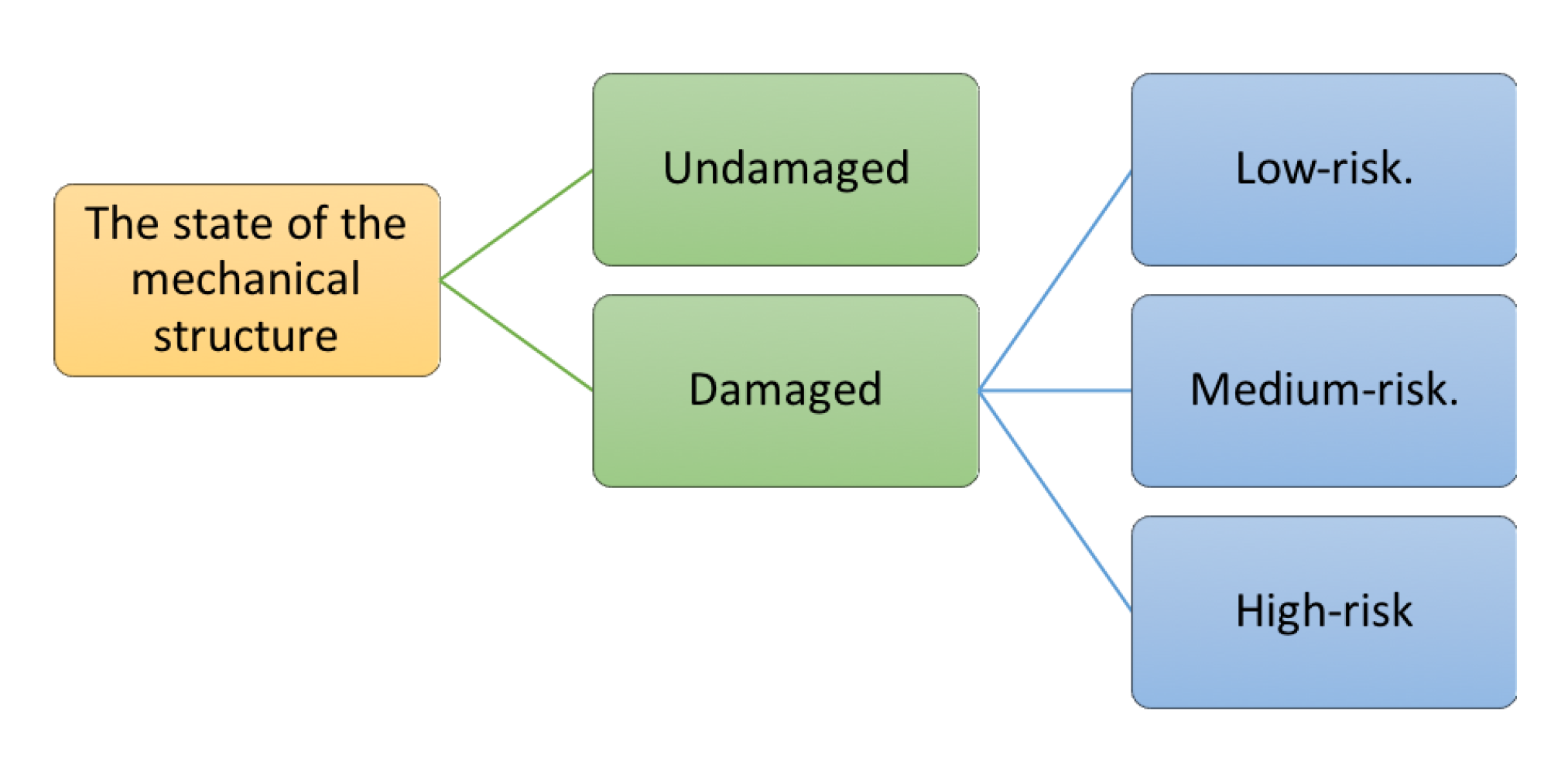
This subsection proposes a neural network-based (NN)-based method for online damage assessment in mechanical structures. The proposed method consists of two cascaded NN models. The first NN model assesses the structural integrity of the system, which is comprised of two classes: the undamaged structure and the damaged structure. The second NN model evaluates the risk level of the damaged structure, which is further identified to belong to one of the following three classes: low-risk, medium-risk, and high-risk. Figure 5 presents the classification hierarchy of the proposed damage assessment method.

3.3.1. Feature Extraction for Machine Learning

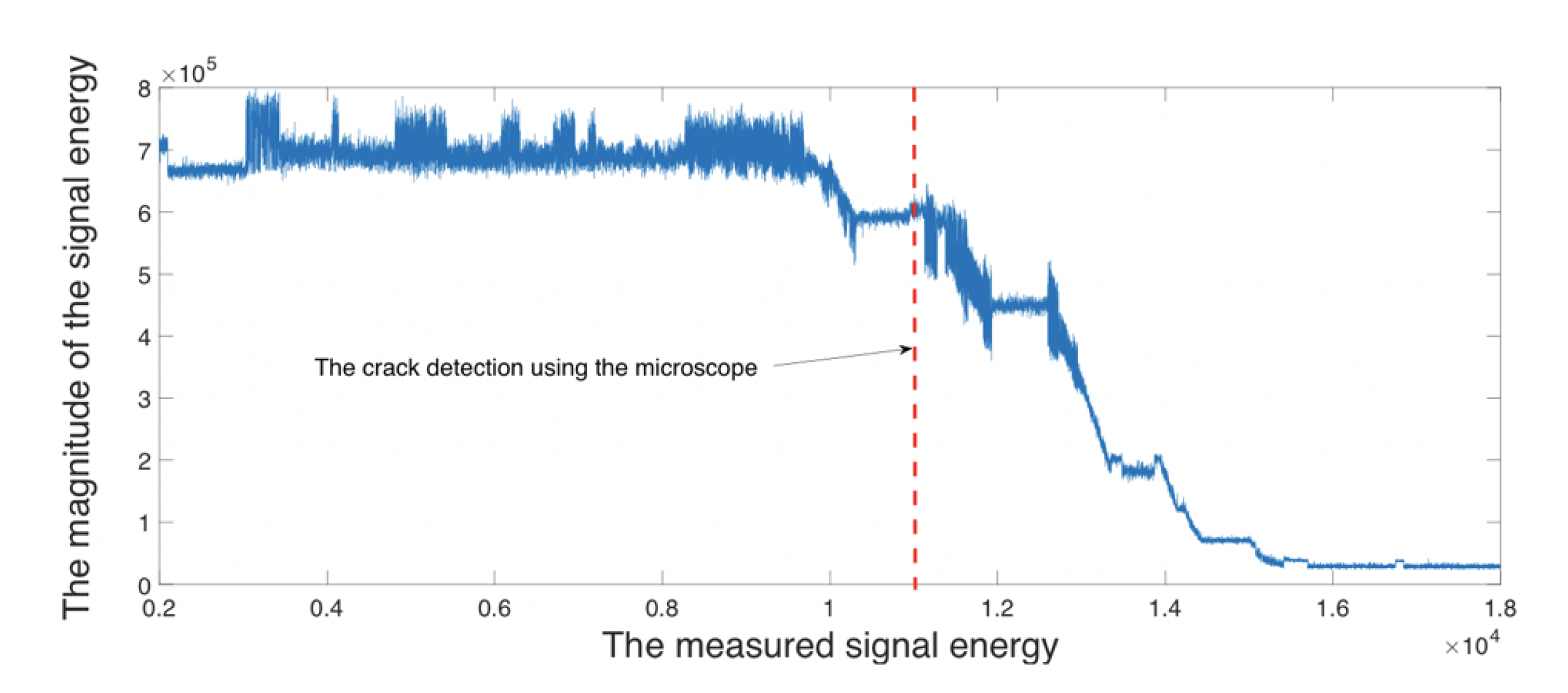
In this paper, the task of feature extraction [29] provides pertinent information (i.e., UT signal attenuation) for detection and classification of fatigue crack damage. The rationale is based on the fact that, for the UT signal, attenuation is a consequence of partial reflection due to the damage evolution (e.g., crack onset). For example, the maximum signal strength implies the undamaged structure (e.g., the fresh test specimen), while the minimum signal strength denotes the damaged structure at the end of its service life (e.g., fully cracked specimen). In the reported work, UT data have been generated synchronously with the images obtained from the digital microscope and confocal microscope (see Figure 1) to provide ground truth for UT signal attenuation; and the signal energy is computed as:

$${\mathit{E}}_{\mathit{\alpha }}={\int }_{-\infty }^{\infty }\mid \mathit{x}\left(\mathit{t}\right){\mid }^{\mathbf{2}}\mathit{dt}$$

(19)

As shown in Figure 6 beyond the vertical red dashed line, the signal energy is significantly attenuated as a consequence of crack evolution. This phenomenon is chosen to be the feature that is used for the classification for the first NN model.

3.3.2. Classification of Damage Patterns

In this paper, the concept of pattern recognition [29,30] has been used for damage detection and classification based on experimental data. In NN, a pattern is a pair of variables $\{\mathit{\varphi },\mathit{\lambda }\}$, where $\mathit{\varphi }$ is a feature vector constructed from measurement data and $\mathit{\lambda }$ is the corresponding label of the feature vector. Along this line, in the reported work, classification procedures have been used for defining pattern allocation criteria for damage assessment. The following two NN models have been constructed for damage detection and risk identification, respectively:

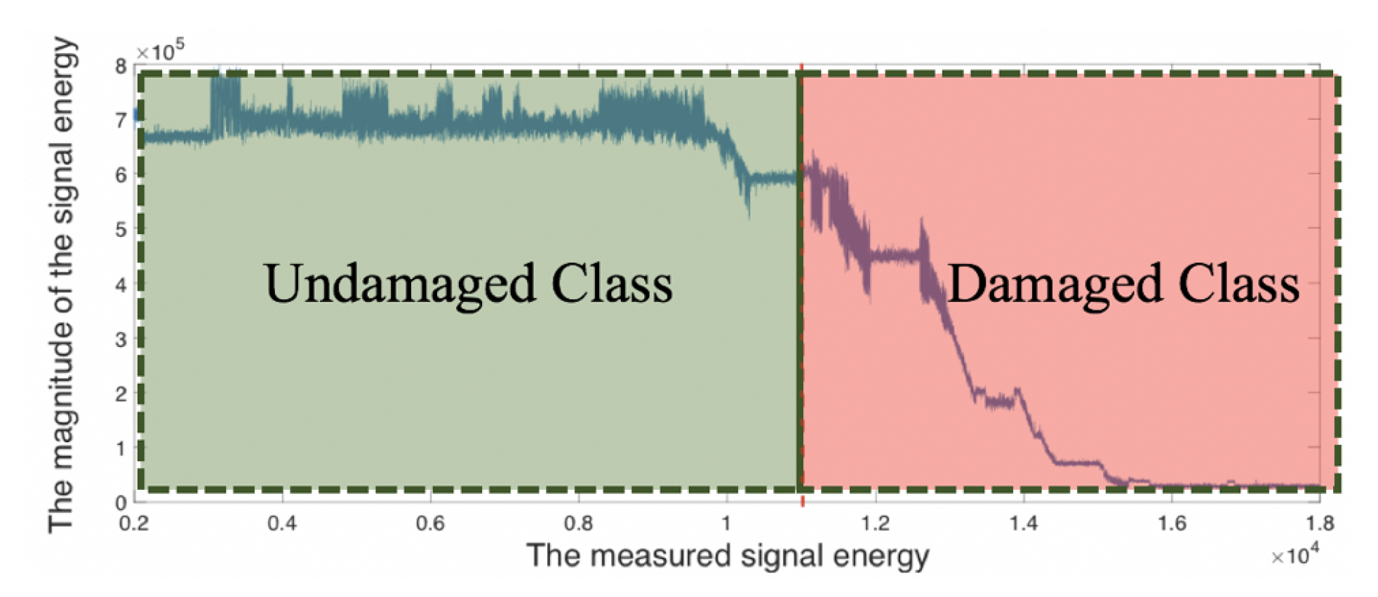
• The first NN model for detection of structural damage: The state of the stressed structure (e.g., a specimen) is classified based on the energy, ${\mathcal{E}}_{\mathit{UT}}$, of UT signals. As seen in Figure 7, before fatigue crack onset (i.e., to the left of the vertical solid line), ${\mathcal{E}}_{\mathit{UT}}$ is labeled to belong to an undamaged class while, after the fatigue crack onset (i.e., to the right of the vertical solid line), ${\mathcal{E}}_{\mathit{UT}}$ is labeled to belong to a damaged class.
• The second NN model for classification of damage risk: The risk of the structural damage (in the damaged class identified by the first NN model) is evaluated based on two criteria. The first criterion is the roughness average (${\mathit{S}}_{\mathit{\alpha }}$) of the investigated area, and the second criterion is the critical crack length ${\mathit{\alpha }}_{\mathit{cr}}$. As seen in Figure 1, a confocal microscope is used to measure the crack tip opening displacement (CTOD) and the roughness average (${\mathit{S}}_{\mathit{\alpha }}$), while the digital microscope is used to measure the crack length $\mathit{\alpha }$. The observations from the confocal microscope and the digital microscope are synchronized such that measurements can be taken simultaneously when the fatigue testing machine is in operation. Following these experimental observations, the damage risk is identified in the following three classes:

  (a)

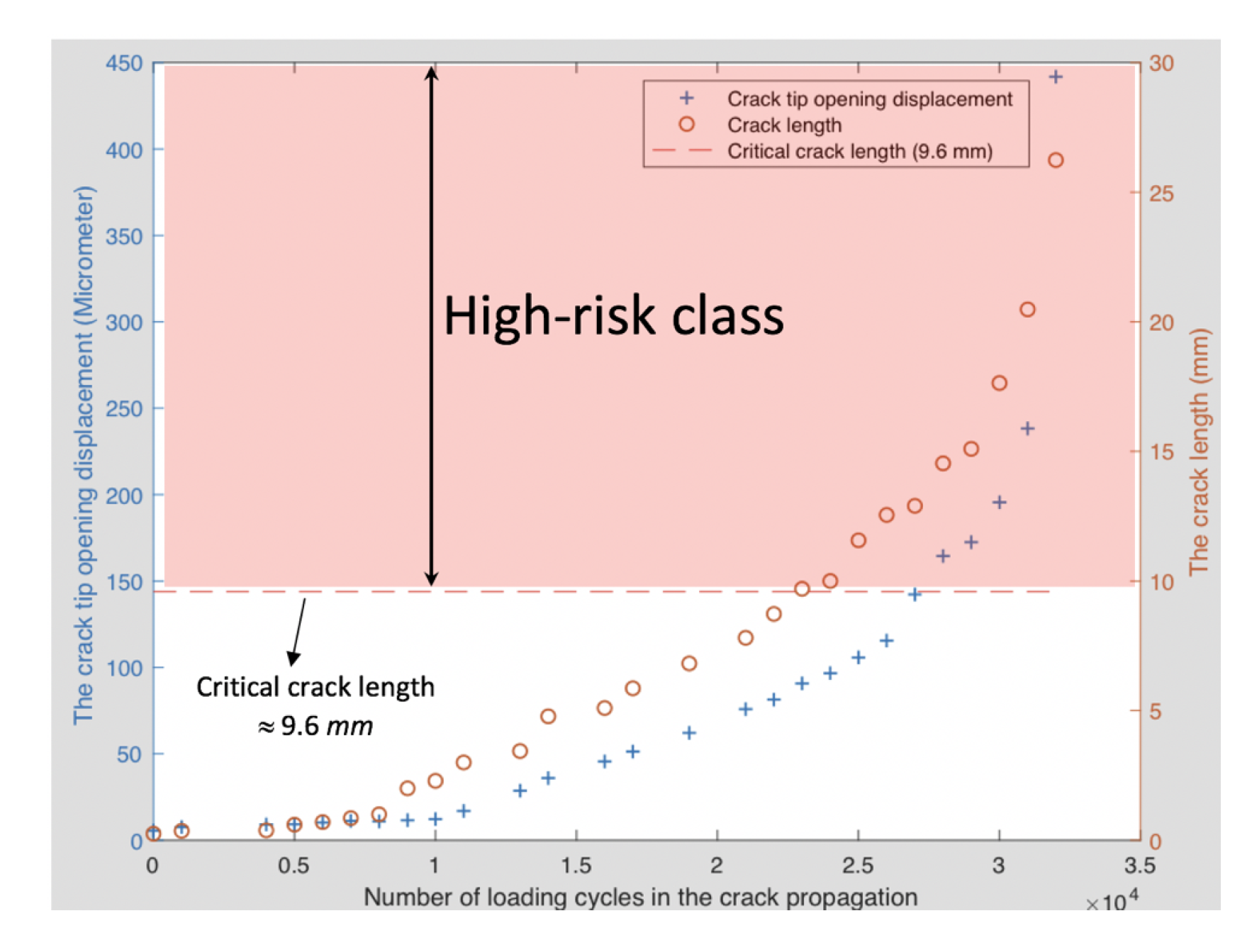
  High-risk damage class: In this class, the critical crack length (CCL) method is applied to determine the damage, in which all measured data after exceeding CCL (${\mathit{\alpha }}_{\mathit{cr}}$) are considered to be of high risk. The critical crack length is computed as:

  $${\mathit{\alpha }}_{\mathit{cr}}=\frac{{\mathit{K}}_{\mathit{IC}}^{\mathbf{2}}}{\mathit{\pi }{\mathit{\sigma }}_{\mathit{max}}^{\mathbf{2}}{\mathit{Y}}_{\mathit{\alpha }}^{\mathbf{2}}}$$

  (20)

  where ${\mathit{K}}_{\mathit{IC}}$ is the fracture toughness (for the Aℓ7075-T6 alloy, ${\mathit{K}}_{\mathit{IC}}$ = 20.0 MPa-${\mathit{m}}^{\mathbf{0}.\mathbf{5}}$); ${\mathit{\alpha }}_{\mathit{cr}}$ is the critical crack length (CCL); ${\mathit{\sigma }}_{\mathit{max}}$ is the maximum applied stress; and the dimensionless parameter ${\mathit{Y}}_{\mathit{\alpha }}$ is computed from the crack length $\mathit{\alpha }$ and specimen width $\mathit{w}$ of the test specimen. For edge cracks in tension, Zahavi et al. [31] introduced the following formula to calculate ${\mathit{Y}}_{\mathit{\alpha }}$.

  $$\begin{array}{c}\hfill {\mathit{Y}}_{\mathit{\alpha }}=\mathbf{1}.\mathbf{12}-\mathbf{0}.\mathbf{231}\left(\frac{\mathit{\alpha }}{\mathit{w}}\right)+\mathbf{10}.\mathbf{55}{\left(\frac{\mathit{\alpha }}{\mathit{w}}\right)}^{\mathbf{2}}-\mathbf{21}.\mathbf{72}{\left(\frac{\mathit{\alpha }}{\mathit{w}}\right)}^{\mathbf{3}}+\mathbf{30}.\mathbf{39}{\left(\frac{\mathit{\alpha }}{\mathit{w}}\right)}^{\mathbf{4}}\end{array}$$

  (21)

  The CCL in all tested specimens is ${\mathit{\alpha }}_{\mathit{cr}}\approx$ 9.6 mm, as seen in Figure 8, where all measurements were taken after reaching CCL and are labeled to belong to the high-risk class.

  (b)

  Medium-risk damage class: As the crack length reaches a certain level, the roughness average (${\mathit{S}}_{\mathit{a}}$) of the investigated area changes dramatically and the crack growth process tends to become unstable; and the effect of the crack on the surface topography becomes noticeable. This change is often called as the ${\mathit{S}}_{\mathit{\alpha }}$_alert. In all experiments, the ${\mathit{S}}_{\mathit{\alpha }}$_alert occurred between the crack onset and CCL. Therefore, all observations of the damage after the ${\mathit{S}}_{\mathit{\alpha }}$_alert and before CCL are classified to belong to the medium-risk class.

  (c)

  Low-risk damage class: The damage observations before CCL are considered to be non-risky. However, this consideration might be ambiguous because the damage risk of observations just before CCL is not similar to that at the damage initiation. Therefore, identifying the damage risk of non-risky damage is very necessary. In the reported work, the roughness average ${\mathit{S}}_{\mathit{\alpha }}$ has been used to quantify the low-risk damage because the effects of tiny cracks on the external surface are, in fact, negligible. In addition, as shown in Figure 9, readings of ${\mathit{S}}_{\mathit{a}}$ before the crack onset are stable, and they are also still stable after the crack onset.

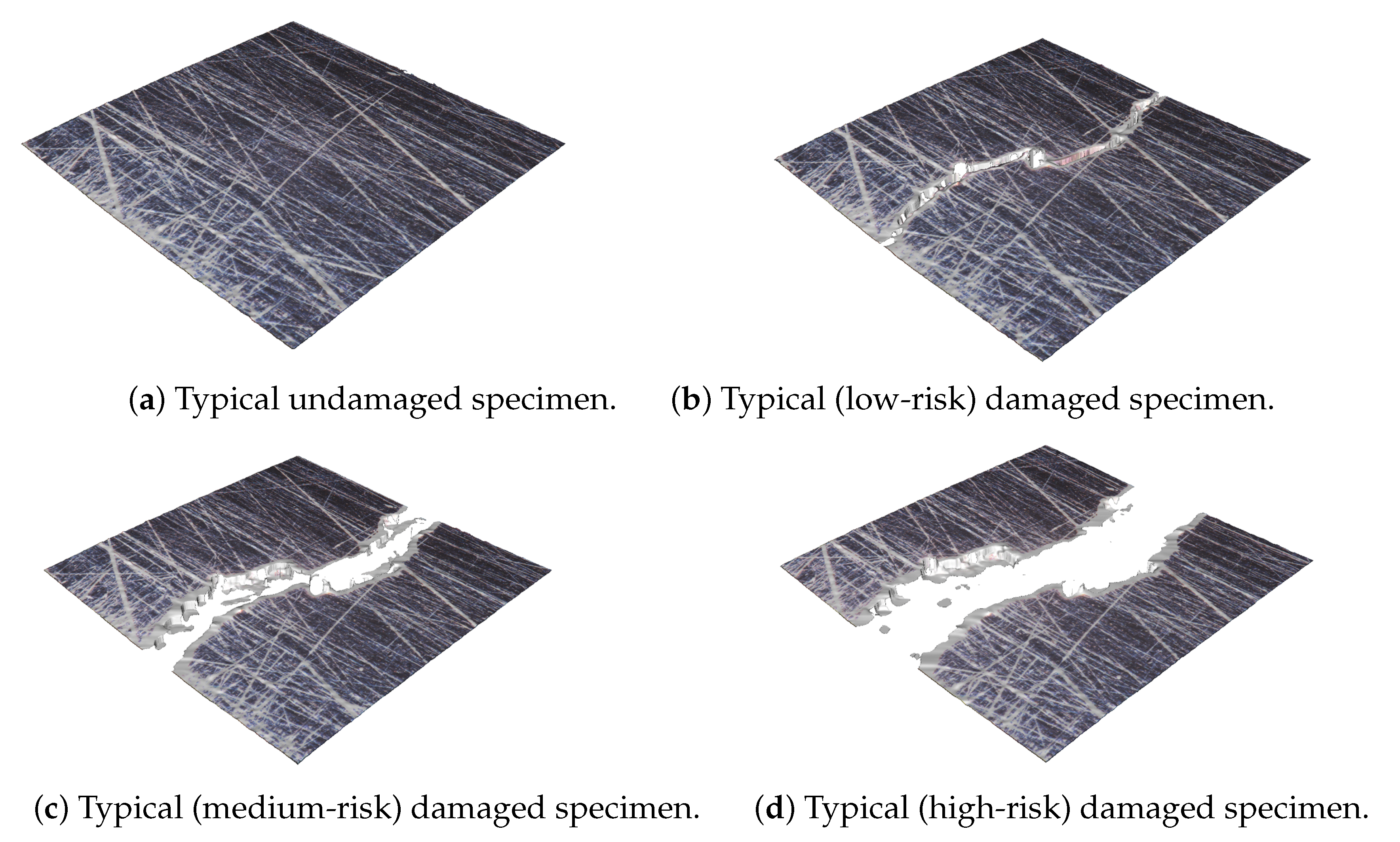
Figure 10a–d present the surface topographies of typical (non-damaged), (low-risk), (medium-risk), and (high-risk) damaged specimens, respectively.

3.3.3. Data Preparation and Neural Networks Procedure

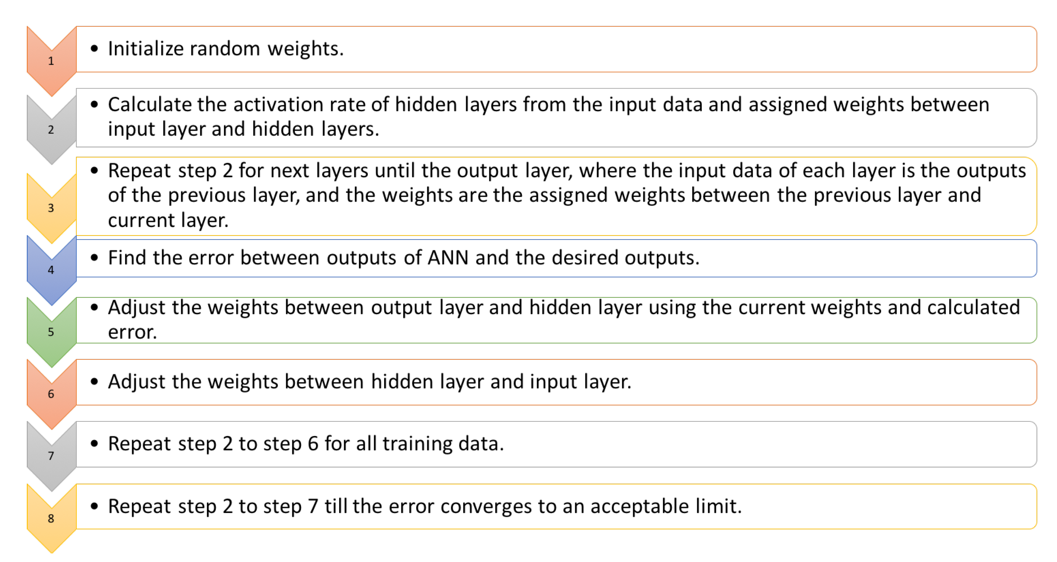
This subsubsection provides the necessary steps for building an NN model with a shallow architecture, as delineated in Figure 11.

In the first NN model, the energy of UT signals is normalized because the response of the signal energy for all tested specimens is of similar texture, but the values of the energy may differ from one to another. The normalization is called a z-score, and it transforms UT signal energy to have a mean of zero and a standard deviation of one. The UT signal energy is normalized as:

$${\mathit{z}}_{\mathit{n}}=\frac{{\mathit{x}}_{\mathit{n}}-\overline{\mathit{x}}}{\mathit{\sigma }}$$

(22)

where $\overline{\mathit{x}}$ is the mean and $\mathit{\sigma }$ is the standard deviation.

In the second NN model, a linear regression model is created relating the relationship between CTOD and CCL to fit the experimental data. The rationale for creating a linear regression model in this paper is as follows:

• Taking CTOD measurements is experimentally expensive, especially at the high-risk level.
• To ensure that the NN model is effective, the training data set must satisfy two conditions: (i) Every group of data must be normalized so that each group pattern is represented in the data set; (ii) statistical deviations must be effectively represented within each class, where both NN models must contain the total range of (noise-corrupted) data [32].

4. Results and Discussion

This section presents and discusses the experimental results for validation of the proposed linear regression and (neural network (NN) models. The first part of this section presents the results of linear regression, while the second part covers the results of NN models.

4.1. Linear Regression Model

As stated in the previous section, before applying the tools of neural network, the amount of the data must be considered, such that every group must contain enough data for training, validating, and testing the neural network model. A selection of the percentage of splitting the dataset into train, validation, and test set depends on the size of the dataset. A common splitting ratio, which is used in this study, is 70% of the data for a train set, 15% for validation set, and 15% for the test set.

In the case of limited data available for training, a regression model that represents typical measurement data can be used, instead of the actual measured data. As seen in Figure 12, a relationship between the crack length (shown as the $\mathit{x}$-axis) and the crack tip opening displacement (CTOD) (shown as the $\mathit{y}$-axis) is built by using a linear regression approach from the experimental data, where the dots represent the actual measured data of an experiment, and the fitted straight line represents the linear regression model.

In Figure 12, the green area presents the low-risk damage class, while the yellow and red areas present the medium-risk and high-risk classes, respectively. Due to the limited amount of available experimental data, it is difficult to have an accurate NN model using the actual measured data. For example, since the medium-risk class has only three measured data, and if one uses the splitting ratio (70% train, 20% test, and 20% validation), either the testing set or validation set will be empty.

Therefore, this problem has been alleviated by incorporating a linear regression model that estimates the CTOD. The linear regression model of Figure 12 is constructed as:

$$\mathit{CTOD}=\mathbf{11}.\mathbf{88}\mathit{a}+\mathbf{1}.\mathbf{186}$$

(23)

where $\mathit{CTOD}$ is the crack tip opening displacement in micrometers, and $\mathit{a}$ is the crack length in $\mathit{mm}$. Furthermore, the size of the input data of the neural network is now increased from 13 measured points to 986 estimated points by using the linear regression model.

4.2. Results Generated from Neural Network Models

This subsection presents the results generated from the two NN models, where the pattern recognition part is handled by the neural network toolbox of MATLAB, which consists of a two-layer feed-forward network, with ten sigmoid hidden neurons (two softmax output neurons for the first model and three softmax output neurons for the second model). The amount of the input data for the first NN model is 19,029 samples, and 986 samples are the inputs for the second NN model.

Table 2. Splitting of input data for training, validation, and testing of the NN models

	The Input Data (Total Samples)	The Training Data (70% Samples)	The Validation Data (15% Samples)	The Testing Data (15% Samples)
First, NN model	19,029	13,321	2854	2854
Second NN model	986	690	148	148

illustrates the splitting of data between the two NN models.

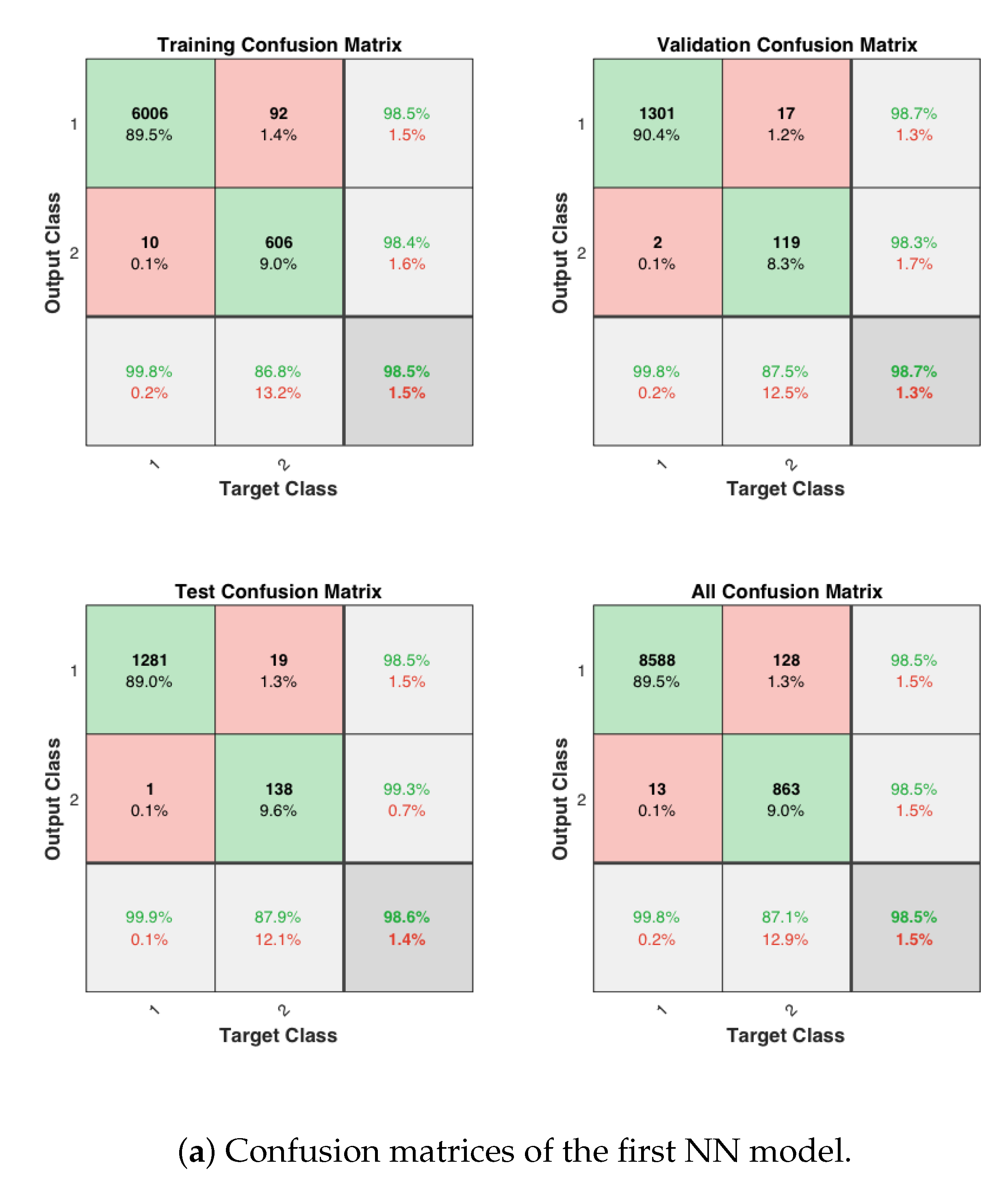
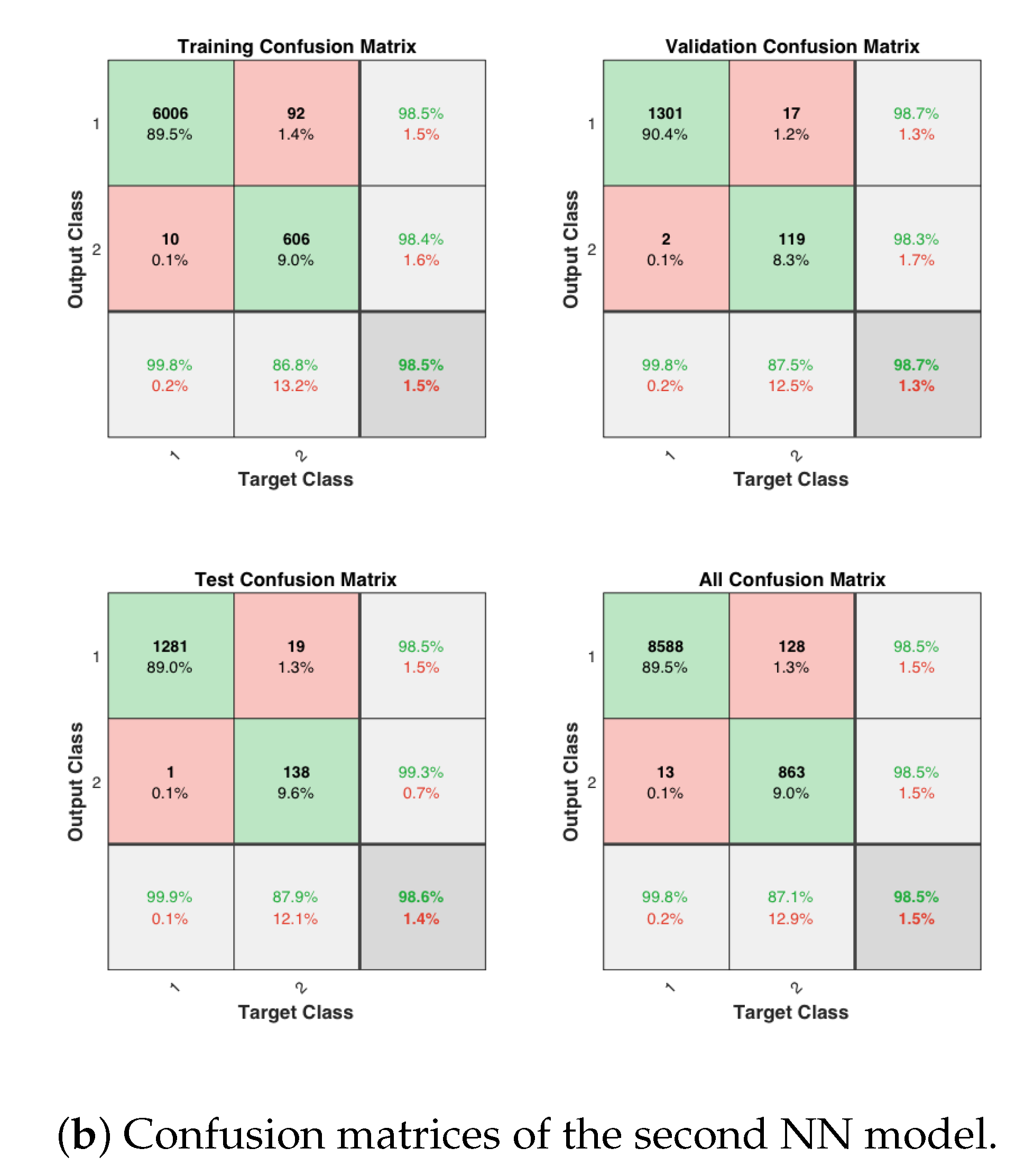
The plates in Figure 13a,b show the confusion matrices of the first NN model and the second NN model, respectively, for training, testing, and overall validation. The outputs of the NN models appear to be very accurate; and the high percentages of correct responses are indicated in the green squares, while the low percentages of incorrect responses appear in the red squares. The lower right gray squares show the overall accuracy/error.

The first NN model, which makes the (binary) detection of undamaged and damaged classes, achieves an accuracy of 98.5% for the training data set, 98.7% for the validation data set, and 98.6% for the testing data set; and the first NN model achieves an overall accuracy of 98.5%. The second NN model, which makes the (trinary) classification of damaged class into high-risk, medium-risk, and low-risk, achieves an accuracy of 95% for the training data set, 94.8% for the validation data set, and 92.8% for the testing data set; and the overall accuracy of the second NN model is equal to 94.6%.

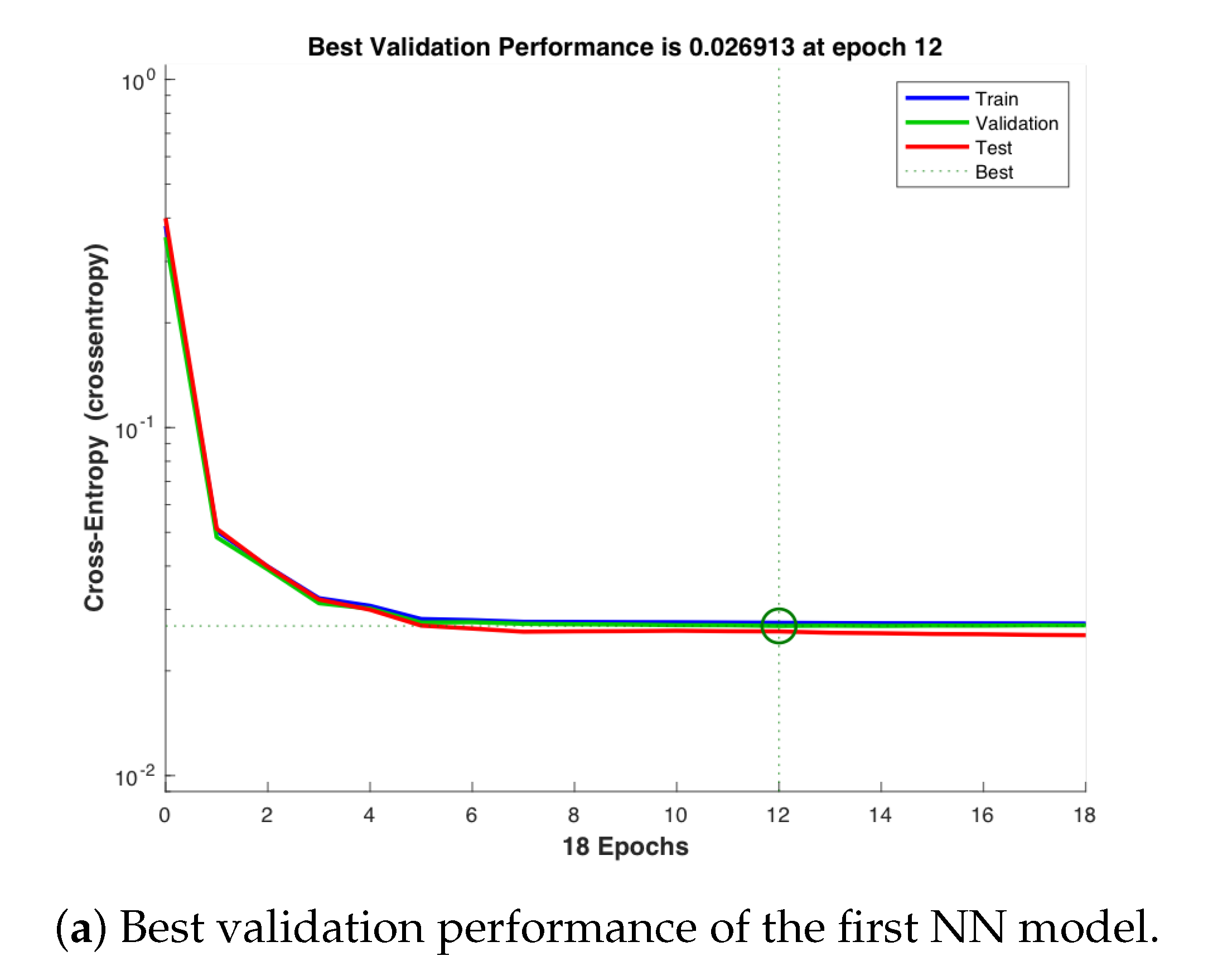
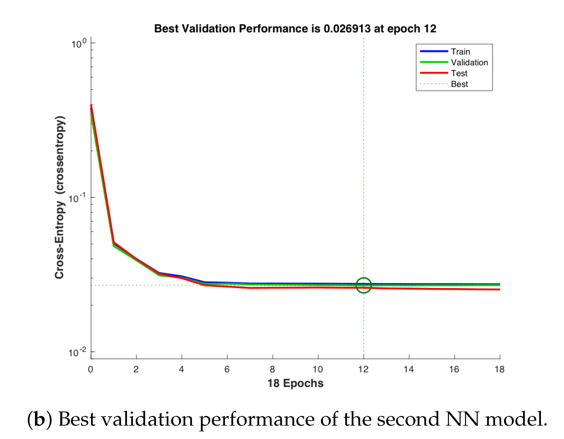
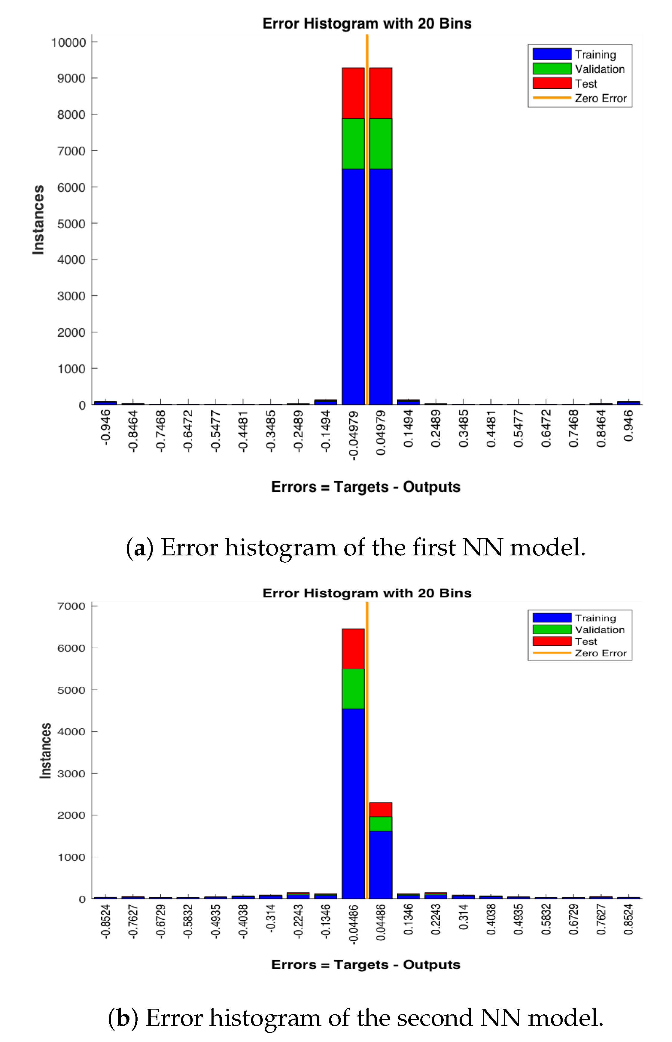
Figure 14a,b show that the best validation performance for the first NN model is achieved at the epoch 12, while that for the second NN model is achieved at the epoch 45. Figure 15a,b illustrate the respective error histograms of the first NN and the second NN models, respectively, for training, validation, and testing. It is noted that the data fitting errors are distributed within a region that is close to the zero-error point.

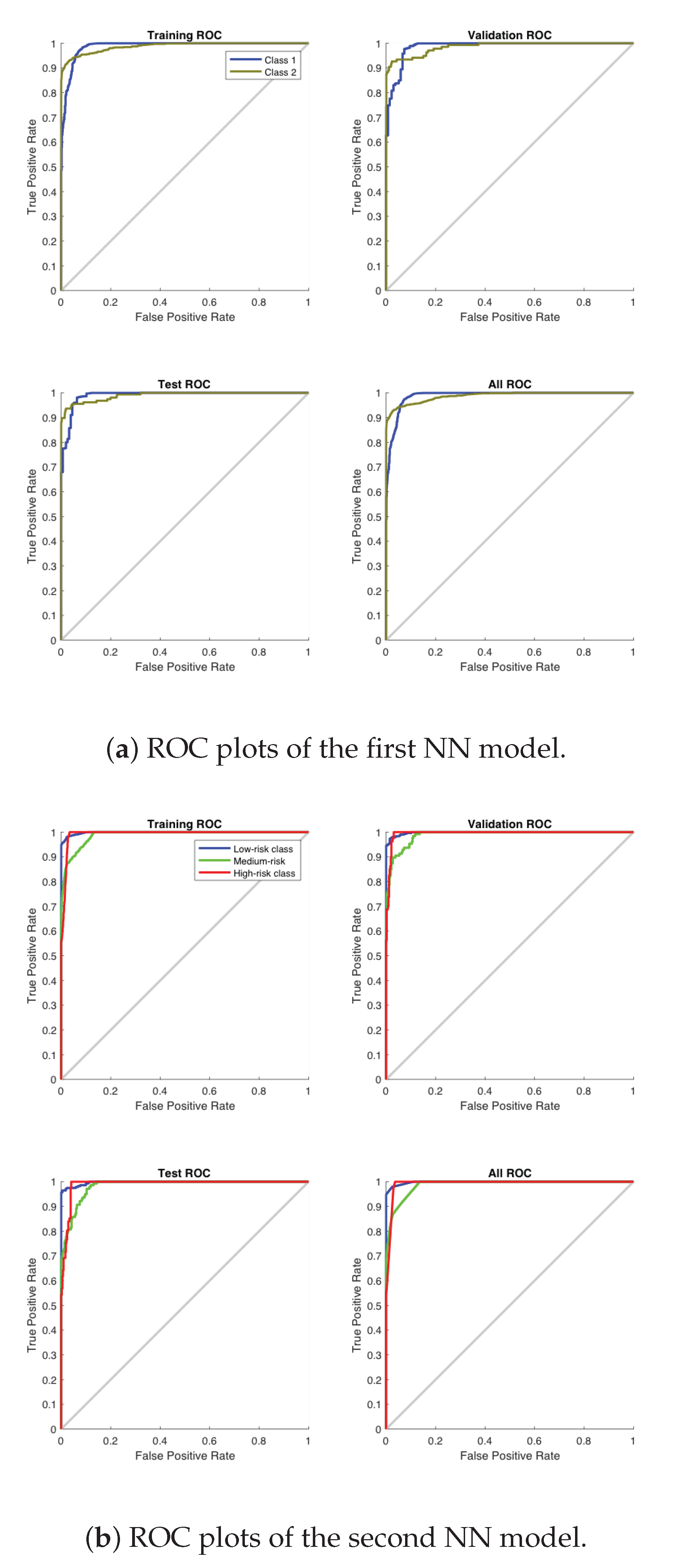
Figure 16a,b show ROC curves (The Receiver Operating Characteristic (ROC) curves [33] have been used in this paper to assess the performance of both NN-based models for damage detection and classification.) for the first NN model and second NN model, respectively, where the colored lines in each figure represent the ROC curves. The ROC curves represent the relationship between the true positive rate of detection (also called sensitivity) on the $\mathit{y}$-axis versus the false positive rate of detection (also called specificity) on the $\mathit{x}$-axis as the threshold is varied. The optimal model (100% sensitivity and 0% specificity) is achieved in the upper-left hand corner. As seen in Figure 16a,b, the performance is excellent for both of the NN models.

5. Summary, Conclusions, and Future Work

This paper has reported the development and experimental validation of a methodology for fatigue-damage assessment in mechanical structures of machinery. The goal is to increase the structural reliability of operating machinery and to avoid grave consequences of the damaged structure, such as endangered safety of plant operating personnel and equipment as well as environmental protection, especially in hazardous engineering applications. For example, real-time assessment of fatigue damage should be applied on petrochemical reactors, where the non-destructive testing (NDT) sensors are embedded in critical locations to provide an updated evaluation for the status of the reactor. Once the fatigue damage is monitored and assessed, human experts should make the final decision on plant operation and maintenance.

In this work, two neural network (NN)-based models have been constructed on the experimental data, acquired from a computer-instrumented and computer-controlled fatigue testing apparatus, equipped with ultrasonic test probes, a confocal microscope, and a digital microscope. It is noted that delicate instruments like optical microscopes are to be used in the laboratory environments only to calibrate the algorithms that make use of (relatively) inexpensive and rugged ultrasonic probes for field applications.

Decision making on damage assessment relies on the outputs of the afore-mentioned two NN models, where the the first model classifies the signal energy of ultrasonic test (UT) data into two classes, namely undamaged class and damaged class; and the second NN model classifies the crack tip opening displacement (CTOD) data into high-risk, medium-risk, and low-risk. Furthermore, a linear regression model has been constructed to augment the amount of the data by estimating the CTOD as inputs to the NN models.

The results of this investigation show that the classification accuracy of the first NN model reaches 98.5%, and that of the second NN model reaches 94.6%. Therefore, the proposed methodology of fatigue-damage assessment systems has the potential of successfully detecting the fatigue damage onset in mechanical structures of machinery and evaluating the associated risk of operation.

While there are many areas of theoretical and experimental research to improve the proposed classification method so that it can be gainfully applied to real-life problems, the following topics are suggested for future research:

• Development of a detailed simulation model of the operating machinery under consideration to generate ample data for training and testing of deep neural networks: This model must be experimentally validated at a few discrete operating points so that the interpolated (and also extrapolated) points of operation are reasonably correct representations of the real-life situations.
• Usage of more advanced tools of neural networks (e.g., convolutional neural networks (CNN) [34] and recurrent neural networks (RNN) [35]) for fatigue-damage assessment: Such advancements are expected to yield wider ranges of applications at the expense of requiring extensive training data.

References

- Farrar, C.R.; Worden, K. Structural Health Monitoring: A Machine Learning Perspective; John Wiley & Sons: Hoboken, NJ, USA, 2012. [Google Scholar]
- Suresh, S. Fatigue of Materials; Cambridge University Press: Cambridge, UK, 1998. [Google Scholar]
- Campbell, F.C. Elements of Metallurgy and Engineering Alloys; ASM International: Almere, The Netherlands, 2008. [Google Scholar]
- Lesiuk, G.; Szata, M.; Rozumek, D.; Marciniak, Z.; Correia, J.; DeJesus, A. Energy response of S355 and 41Cr4 steel during fatigue crack growth process. J. Strain Anal. Eng. Des. 2018, 53, 663–675. [Google Scholar] [CrossRef]
- Meruane, V.; Mahu, J. Real-time structural damage assessment using artificial neural networks and antiresonant frequencies. Shock Vib. 2014, 2014, 653279. [Google Scholar] [CrossRef]
- Meruane, V.; Heylen, W. An hybrid real genetic algorithm to detect structural damage using modal properties. Mech. Syst. Signal Process. 2011, 25, 1559–1573. [Google Scholar] [CrossRef]
- Meruane, V.; Heylen, W. Damage detection with parallel genetic algorithms and operational modes. Struct. Health Monit. 2010, 9, 481–496. [Google Scholar] [CrossRef]
- Dervilis, N. A Machine Learning Approach to Structural Health Monitoring with a View towards Wind Turbines. Ph.D. Thesis, University of Sheffield, Sheffield, UK, 2013. [Google Scholar]
- Güemes, A.; Fernandez-Lopez, A.; Pozo, A.R.; Sierra-Pérez, J. Structural Health Monitoring for Advanced Composite Structures: A Review. J. Compos. Sci. 2020, 4, 13. [Google Scholar] [CrossRef]
- Dong, T.; Haftka, R.T.; Kim, N.H. Advantages of Condition-Based Maintenance over Scheduled Maintenance using Structural Health Monitoring System. In Reliability and Maintenance—An Overview of Cases; IntechOpen: London, UK, 2019. [Google Scholar]
- Friedmann, H.; Kraemer, P. Vibration-based condition monitoring, structural health monitoring, population monitoring–Approach to a definition of the different concepts by means of practical examples from the field of wind energy. In Proceedings of the 8th European Workshop on Structural Health Monitoring (EWSHM 2016), Bilbao, Spain, 5–8 July 2016. [Google Scholar]
- Gonzalez-Perez, C.; Valdes-Gonzalez, J. Identification of structural damage in a vehicular bridge using artificial neural networks. Struct. Health Monit. 2011, 10, 33–48. [Google Scholar] [CrossRef]
- Arangio, S.; Beck, J. Bayesian neural networks for bridge integrity assessment. Struct. Control. Health Monit. 2012, 19, 3–21. [Google Scholar] [CrossRef]
- Strączkiewicz, M.; Barszcz, T. Application of artificial neural network for damage detection in planetary gearbox of wind turbine. Shock Vib. 2016, 2016. [Google Scholar] [CrossRef]
- Danzl, R.; Helmli, F.; Scherer, S. Comparison of roughness measurements between a contact stylus instrument and an optical measurement device based on a colour focus sensor. In Technical Proceedings of the 2006 NSTI Nanotechnology Conference and Trade Show; CRC Press: Boca Raton, FL, USA, 2006; pp. 284–287. [Google Scholar]
- Danzl, R.; Helmli, F.; Scherer, S. Focus variation—A robust technology for high resolution optical 3D surface metrology. Stroj.-Vestn.-J. Mech. Eng. 2011, 57, 245–256. [Google Scholar] [CrossRef]
- Abazid, M.; Alkoud, D. A Least-Squares Approach to Prediction The Future Sales of Pharmacy; Blue Eyes Intelligence Engineering & Sciences Publication Pvt. Ltd.: Bhopal, India, 2018. [Google Scholar]
- Mallick, P.; Nayak, C.; Behera, T. Least square based parabolic regression to determine calibration constant in measurement. In Proceedings of the 2010 5th International Conference on Industrial and Information Systems, Mangalore, India, 29 July–1 August 2010; pp. 334–338. [Google Scholar]
- Wang, Z.; Yan, W.; Oates, T. Time series classification from scratch with deep neural networks: A strong baseline. In Proceedings of the 2017 International Joint Conference on Neural Networks (IJCNN), Anchorage, AK, USA, 14–19 May 2017; pp. 1578–1585. [Google Scholar]
- Coolen, A.C. A beginner’s guide to the mathematics of neural networks. In Concepts for Neural Networks; Springer: Berlin/Heidelberg, Germany, 1998; pp. 13–70. [Google Scholar]
- Zakaria, M.; Al-Shebany, M.; Sarhan, S. Artificial neural network: A brief overview. Int. J. Eng. Res. Appl. 2014, 4, 7–12. [Google Scholar]
- Islam, M.; Chen, G.; Jin, S. An Overview of Neural Network. Am. J. Neural Netw. Appl. 2019, 5, 7–11. [Google Scholar] [CrossRef]
- Zayegh, A.; Al Bassam, N. Neural network principles and applications. In Digital Systems; IntechOpen: London, UK, 2018. [Google Scholar]
- Wang, X. Method of steepest descent and its applications. IEEE Microw. Wirel. Compon. Lett. 2008, 12, 24–26. [Google Scholar]
- Ruder, S. An overview of gradient descent optimization algorithms. arXiv 2016, arXiv:1609.04747. [Google Scholar]
- Møller, M.F. A scaled conjugate gradient algorithm for fast supervised learning. Neural Netw. 1993, 6, 525–533. [Google Scholar] [CrossRef]
- Bishop, C.M. Pattern Recognition and Machine Learning; Springer: Berlin/Heidelberg, Germany, 2006. [Google Scholar]
- Dkhichi, F.; Oukarfi, B. Neural Network Training By Gradient Descent Algorithms: Application on the Solar Cell. Int. J. Innov. Res. Sci. Eng. Technol. 2014, 3, 15696–15702. [Google Scholar] [CrossRef]
- Ghorpade, S.; Ghorpade, J.; Mantri, S. Pattern recognition using neural networks. Int. J. Comput. Sci. Inf. Technol. (IJCSIT) 2010, 2, 92. [Google Scholar] [CrossRef]
- Ghotkar, V.N.; Indurkar, P.; Chilke, B. The Pattern Recognition using Spiking Neural Network and Neural Network. Int. J. 2015, 5. [Google Scholar]
- Zahavi, E.; Torbilo, V.; Press, S. Fatigue Design: Life Expectancy of Machine Parts; CRC Press: Boca Raton, FL, USA, 1996. [Google Scholar]
- Thirumalainambi, R.; Bardina, J. Training data requirement for a neural network to predict aerodynamic coefficients. In Proceedings of the Independent Component Analyses, Wavelets, and Neural Networks. International Society for Optics and Photonics, Orlando, FL, USA, 1 April 2003; Volume 5102, pp. 92–103. [Google Scholar]
- Poor, H. An Introduction to Signal Detection and Estimation; Spriger: New York, NY, USA, 1994; p. 308. [Google Scholar]
- Alqahtani, H.; Bharadwaj, S.; Ray, A. Classification of fatigue crack damage in polycrystalline alloy structures using convolutional neural networks. Eng. Fail. Anal. 2021, 119. [Google Scholar] [CrossRef]
- Husken, M.; Stagge, P. Recurrent neural networks for time series classification. Neurocomputing 2003, 50, 223–235. [Google Scholar] [CrossRef]
Figure 1.
The fatigue testing apparatus and ancillaries; in (b), all dimensions are in mm.
Figure 2.
Three different types of neural network architecture.
Figure 3.
An artificial neuron.
Figure 4.
The sigmoid function.
Figure 5.
The classification hierarchy.
Figure 6.
The UT signals energy for one experiment, where the -axis presents 19,029 UT energy measurements during each experiment; and the -axis shows the value of measured signal energy.
Figure 7.
The The classification of the first stage, the damage initiation.
Figure 8.
Determining the high-risk region using the crack length and CTOD.
Figure 9.
The average surface roughness, , measurements of one experiment.
Figure 10.
Illustration of fatigue-damage evolution in a typical test specimen.
Figure 11.
The neural network analysis procedure.
Figure 12.
The linear regression model of the crack length and the crack tip opening displacement.
Figure 13.
Performance of the first and second neural network models for all experiments.
Figure 14.
Best validation performance for all experiments.
Figure 15.
Error histogram for all experiments.
Figure 16.
Receiver operating characteristics (ROC) for all experiments.