Article

Sensorless Control of Permanent Magnet Synchronous Machine with Magnetic Saliency Tracking Based on Voltage Signal Injection †

by
Vasilios C. Ilioudis
Department of Industrial Engineering and Management, International Hellenic University (IHU), 57400 Thessaloniki, Greece
This paper is an extended version of our paper published in “Vasilios C. Ilioudis. Sensorless Control Applying Signal Injection Methodology on Modified Model of Permanent Magnet Synchronous Machine published in 2019 6th International Conference on Control, Decision and Information Technologies (CoDIT), Paris, France 23–26 April 2019.
Machines 2020, 8(1), 14; https://doi.org/10.3390/machines8010014
Submission received: 7 February 2020 / Revised: 9 March 2020 / Accepted: 9 March 2020 / Published: 19 March 2020

Abstract

:
This paper presents a sensorless control method of a permanent magnet synchronous machine (PMSM) with magnetic saliency estimation. This is based on a high-frequency injection (HFI) technique applied on the modified PMSM model in the γδ reference frame. Except for sensorless control, an emphasis is placed on the magnetic saliency estimation to indicate a practical approach in tracking PMSM inductance variations. The magnetic saliency is determined using calculations embedded in the speed and position algorithm through current measurements. A notable characteristic of the modified PMSM model is that the corresponding rotor flux integrates both permanent magnet and saliency term fluxes. In applying a HFI technique for sensorless control, the structure of the PMSM flux model is formatted accordingly. A novel inductance matrix is derived that is completely compatible with the HFI methodology, since its elements include terms of angle error differential and average inductances. In addition, a sliding mode observer (SMO) is designed to estimate the speed and angle of rotor flux based on equivalent control applying a smooth function of the angle error instead of a sign one to reduce the chattering phenomenon. The control strategy is principally based on the adequacy of the proposed modified model and on the appropriateness of the SMO structure to successfully track the rotor flux position with the required stability and accuracy. Simulation results demonstrate the performance of the PMSM sensorless control verifying the effectiveness of the proposed algorithm to detect PMSM saliency, speed and position in steady state and transient modes successfully.

Notation

  • ud, uq = dq axis stator voltages
  • id, iq = dq axis stator currents
  • λd, λq = dq axis stator magnetic fluxes
  • λm = rotor magnetic flux
  • Ld, Lq = dq axis inductances
  • ΣL =(Ld+Lq)/2 = average inductance
  • ΔL = (Ld-Lq)/2 = differential inductance
  • rs = stator resistance
  • uγ, uδ= γδ axis stator voltages
  • iγ, iδ= γδ axis stator currents
  • λγ, λδ= γδ axis stator magnetic fluxes
  • p = number of pole pairs
  • θ = θe = electrical angular position
  • ω = ωe = electrical angular speed

1. Introduction

Permanent magnet synchronous machines (PMSM) are used to an increasing rate in a wide rage of industrial applications due to their very appealing properties. Among them are the high efficiency and dynamics, the high torque inertia ratio, the small size and the very low torque ripple. For internal PMSM (IPMSM) in particular, low or even zero-speed sensorless operation is feasible, while field weakening allows extension of operation at speeds above the nominal. Efficient operation of synchronous machines implies very low energy losses compensating their higher initial cost. In a high-performance PMSM operation, advanced control methods are applied, such as field oriented control (FOC), aiming to achieve smooth rotation over the entire speed range, fast response and full torque control [1,2]. However, these PMSM control methods need an accurate rotor position to fulfil these control requirements. Typically, rotor position sensors, such as optical encoders or magnetic resolvers are used to directly perform rotor angle measurement. Nevertheless, the mounted sensors increase the total cost and mainly introduce noise reducing the reliability of the implemented control particularly in electrically hostile environment. As a consequence, an increasing interest was created in sensorless control techniques that have the aim of employing indirect techniques for the rotor position estimation instead of using mechanical sensors.
In the literature, a plethora of PMSM sensorless approaches have been proposed that could be mainly classified into two strategies: the fundamental excitation and saliency and signal injection [3,4,5,6,7]. The first strategy has been established based on the state observer methodology using only measurements of fundamental excitation variables such as stator voltages and currents. Appropriately designed back electromotive force (back-EMF or BEMF) or magnetic flux observers estimate the rotor position and speed information [8,9,10,11,12]. In particular, the back-EMF estimation methods are normally capable of providing accurate positions in a limited speed range from the middle to high-speeds [1]. At low speed range, the induced back-EMF is relatively very small degrading seriously the estimation accuracy, since the amplitude of back-EMF is comparable to the added measurement noise [1,2,13]. By contrast with a fundamental strategy, the saliency and signal injection-based methods are applied to detect rotor flux position by means of PMSM spatial inductance variations. At low speed range even at zero speed operation, a rotor position can be accurately estimated through injecting voltage signals of high frequency, as it is shown in Figure 1 [4,5,6,14,15]. This PMSM sensorless strategy is based on the rotor magnetic anisotropy or on the presence of magnetic saliency, i.e., (Ld − Lq) ≠ 0. Although high-frequency injection (HFI) methods are very efficient in terms of angle estimation accuracy, the control performance is strongly affected by the PMSM magnetic, mechanical parameters and the mathematical model used. Furthermore, the injected high-frequency signal may introduce a considerable audible noise that could not be tolerable [16]. Moreover, the proposed PMSM model plays a key role in the proposed sensorless approach. Since the rotor position cannot be detected, the d–q axis mathematical model cannot be applied directly. Most approaches are based on the estimation of the PMSM variables such as the back electromotive force, in the stationary reference frame αβ. In a typical sensorless control scheme, the rotor speed and position are obtained from estimated PMSM parameters or variables, such as back-EMF or rotor flux, implementing state estimators such as a Luenberger, sliding mode or phase-locked-loop (PLL)-type observer [4,17]. Several developed observers were based on PMSM current model, which may cause instability issues in some speed ranges due to introduced model assumptions [4,17]. In avoiding such model simplifications, the magnetic saliency and the back-EMF terms are included into the so-called extended EMF [1,18,19]. However, the observers in the αβ stationary reference frame suffer from phase delay between the real and the estimated EMF, since the real extended EMF is a sinusoidal signal [18,20]. This undesired phase delay is due to the observer operation, which is similar to signal filtering. Despite the αβ stationary frame, PMSM variables, such as flux and extended EMF, are constant quantities in the dq (direct-quadrature) synchronous rotating reference frame that, however, cannot be applied directly. An advantageous alternative proposal is to express PMSM mathematical model in the γδ reference frame, which is rotating at estimated angular velocity ω ^ and lagging behind the dq synchronous reference frame by electrical angle θ ¯ , i.e., the angle difference between dq and γδ (see Figure 2) [1,21,22]. Among the benefits gained from transforming the PMSM model to γδ reference frame is its suitability for sensorless control allowing the estimation of variables in a rotating frame rather than in stationary frame. Particularly, the γδ-modified model is more convenient regarding the magnetic saliency and it could be applied on both salient-pole (Ld ≠ Lq) and nonsalient-pole PMSM (Ld = Lq = Ls) [1,21]. Observers developed in the γδ reference frame are able to provide the angle error θ ¯ between dq and γδ reference frames instead of the rotor angle θ. In addressing the phase delay issue, the PMSM model in the γδ reference frame is preferable, since the γδ frame is associated with the rotor flux. As a result, the phase delay between dq and γδ variables is very small considered as negligible [1].
Typically, PMSM are classified into two common types of permanent magnet (PM) machines, namely the surface permanent magnet synchronous machine (SPMSM or SPM) and internal permanent magnet synchronous machine (IPMSM or IPM). The magnetic saliency of a machine is defined as the difference between d-axis and q-axis inductances, i.e., (Ld − Lq). In SPMSM, the magnets are mounted on the surface of the rotor, whereas the magnets of IPMSM are buried inside the rotor. Since the permeability of permanent magnets is very low, it can be considered as equal to the air permeability along the flux paths. Therefore, the effective air gap remains the same in the magnetic flux paths of the d-axis and q-axis for SPMSM [23]. As a result, the inductance measured at the machine terminal is constant regardless of the rotor position, i.e., Ld = Lq, implying that the magnetic saliency of SPMSM is zero or very low, i.e., (Ld − Lq) ≅ 0. In contrast, the effective air gap in the magnetic flux path of IPMSM differs between the d-axis and q-axis depending on the rotor position, since the permanent magnets have lower permeability than iron. Hence, the machine inductance fluctuates implying a magnetic saliency different than zero, i.e., (Ld − Lq) ≠ 0. Measuring the inductance changes allows the estimation of rotor position. As a result, it is possible to detect the rotor position using inductance saliency (sensorless control or open speed control loop) [24,25,26]. On the other hand, the quantification of PMSM magnetic saliency is a very complex and difficult problem requiring data analysis of experimental measurements or finite element methods (FEM). Mainly, the inductance variance is associated with the magnetic saturation or rotor geometric saliency, which are the most common sources of magnetic saliency. Besides these, the rotor eccentricity, the eddy currents and the slotting of the rotor and stator may also cause magnetic saliency [15,23,24]. In dq axes, the synchronous inductances can be expressed as the sum of the leakage and magnetizing inductances, i.e., Ld = Lld + Lmd, Lq = Llq + Lmq, where Lld, Llq are leakage inductances and Lmd, Lmq represent the magnetizing inductances. Leakage inductances are associated with the slots, teeth and faces’ magnetic leakage, while magnetizing inductances are associated with the main magnetic flux passing through the air gap. Considering magnetic saturation and rotor geometric saliency, both of them influence the leakage and the magnetizing inductances [15,24,25,26]. The signal injection methods are able to detect both types of saliencies with injecting frequencies usually in the range from 0.5 kHz to 2 kHz [27]. However, the high-frequency injection may decrease the precision of estimation due to the current controller bandwidth limitations in a closed loop. Therefore, it is preferable to generate the harmonic voltage injection in the inverter stage [23].
In this work, a new mathematical model of PMSM is proposed expressed in a modified form for rotor flux equations and referred to the γδ estimated rotating frame. The PMSM model in γδ is much more convenient for sensorless control methods including the saliency and signal injection strategies [21]. The development of the PMSM modified model in γδ and the change of the stator flux to obtain a novel stator inductance matrix Lγδ constitute the main theoretical contributions of the present study. Saliency depended terms, such as (Ld − Lq)id, are embedded into the modified rotor flux in γδ allowing minimization the PMSM model approximations. Despite of the extended EMF or saliency back-EMF model, the modified γδ model is advantageous, since speed has no effect on the modified rotor flux instead [1,12,21,28,29]. As is proven, the γδ inductance matrix Lγδ is transformed from the original Ldq based on the angle difference between dq and γδ. In particular, it is also proven that the elements of the γδ inductance matrix Lγδ are functions of the average inductance, the differential inductance and angle error. This property is of great importance, since the presented analysis of the derived matrix Lγδ verifies the appropriateness of the γδ reference frame in the design procedure. Due to the injection of the high frequency voltage, the resulting high-frequency (HF) stator current contains two components with positive and negative frequencies, i.e., current vectors rotate in opposite directions. After appropriate processing and filtering, the PMSM rotor position information is extracted through a sliding mode observer (SMO) employing the equivalent control methodology [30]. Since chattering avoidance is important in sliding mode applications, the sgn(.) function is substituted by the smooth function tanh(.). Such a continuous approximation is very efficient allowing considerable reduction of chattering effect. Also, a notable advantageous property of the proposed solution is that the PMSM stator inductances in dq and magnetic saliency (Ld − Lq) = 2ΔL can be reliably calculated based on the magnitudes of the derived HF current components. Figure 1 presents in details the total control scheme based on the γδ modified model of PMSM aiming to estimate the rotor speed and position and calculate magnetic saliency. The present sensorless control includes the measurement, the estimation and the control phases. In the measurement phase, only the stator currents ia and ib are needed. Estimation of rotor speed and angle is curried out at observer after processing the current signals (modulation, low-pass filter (LPF) and band-pass filter (BPF)). The desired control is implemented using tree proportional-integral controllers: two for current control (inner loops) and one for speed control (outer loop). Injection succeeds adding the HF voltage signals to the γδ voltage components derived from current controllers. After obtaining the reference voltages uα* and uβ*, a voltage source inverter (VSI) produces the desired voltage to feed the PMSM by means of appropriate modulation, such as Space Vector Pulse Width Modulation (SVPWM). The evolved algorithm permits the accurate speed/position estimation and on-line calculation of stator impedances and saliency for monitoring or fault detection [31,32,33,34,35]. Finally, Simulink/Matlab is used to examine and evaluate the proposed algorithm indicating very satisfactory results.
The rest of the paper is organized as follows. In Section 2, an analysis of the modified PMSM model is presented in dq and γδ reference frame emphasizing in inductance matrix and magnetic saliency. The high-frequency injection and rotor speed and position observer is described in Section 3. In deriving the stator inductances and saliency, the relations between filtered current signals are analyzed in Section 4. Simulation set-up and results are presented and discussed in Section 5, while Section 6 concludes the presented work.

2. Analysis of Modified Permanent Magnet Synchronous Machine (PMSM) Model

2.1. Modified PMSM Voltage and Flux/Current Model in Synchronous Reference Frame dq

The PMSM mathematical model depends mainly on the type, i.e., IPMSM or SPMSM, the geometric properties, and the reference frame used. In next paragraphs, a salient-pole permanent magnet (PM) synchronous machine is considered, where the air gap of the flux path is varying due to the presence of magnetic saliency, LdLq, and the induced back EMF (BEMF) is sinusoidal. The following equations express the PMSM model in the synchronous reference frame dq:
u d q = r s i d q + ω J s λ d q + λ ˙ d q ,
λ d q = L d q i d q + λ m d q ,
where
i d q = [ u d u q ] ,   λ d q = [ λ d λ q ] ,   J s = [ 0 1 1 0 ] ,   L d q = [ L d 0 0 L q ]   and   λ m d q = [ λ m 0 ] ,
Considering the magnetic saliency term (Ld − Lq), the flux terms of the PMSM model in dq could be expressed in a symmetric form, i.e., the stator flux matrix λdq in Equation (2) can be equivalently rewritten as:
λ d q = [ L q 0 0 L q ] [ i d i q ] + [ λ m + ( L d L q ) i d 0 ] = [ L q 0 0 L q ] [ i d i q ] + [ λ m m 0 ] = L q q i d q + λ m m d q ,
Here, the λmm is defined as the PMSM modified rotor flux in dq, which depends on the permanent magnet flux λm, the magnetic saliency (Ld − Lq), and the d-axis stator current id (see Figure 2). In practice, for small id currents, the modified rotor flux λmm is mainly dominated by λm.

2.2. Modified PMSM Voltage and Flux/Current Model in γδ

The modified rotor flux vector is schematically shown in Figure 2 for αβ, dq and γδ reference frames. By definition, the γδ reference frame is an arbitrary reference frame, which is rotating at an estimated angular velocity ω ^ and lagging behind the dq reference frame by the electrical angle determined as Δ θ = θ ¯ = θ θ ^ [1,19]. The γδ PMSM model is obtained through transforming the corresponding dq model by means of the transformation matrix KΔθ defined in Equation (5), which depends on the angle difference between the dq and γδ rotating reference frames [1,21].

2.3. Modified PMSM Voltage and Flux/Current Model in γδ

The modified rotor flux vector is schematically shown in Figure 2 for αβ, dq and γδ reference frames. By definition, the γδ reference frame is an arbitrary reference frame, which is rotating at an estimated angular velocity ω ^ and lagging behind the dq reference frame by the electrical angle determined as Δ θ = θ ¯ = θ θ ^ [1,21]. The γδ PMSM model is obtained through transforming the corresponding dq model by means of the transformation matrix KΔθ defined in Equation (5), which depends on the angle difference between the dq and γδ rotating reference frames [1,21],
K Δ θ = [ cos θ ¯ sin θ ¯ sin θ ¯ cos θ ¯ ] ,
Multiplying from the left both parts of Equations (1), (4) by KΔθ, the γδ model of PMSM for stator voltage and flux is written as follows:
K Δ θ u d q = K Δ θ r s i d q + K Δ θ ω J s λ d q + K Δ θ λ ˙ d q u γ δ = r s i γ δ + ω J s λ γ δ + ( θ ¯ ˙ J s λ γ δ + λ ˙ γ δ ) u γ δ = r s i γ δ + ω J s λ γ δ + ( θ ¯ ˙ J s λ γ δ + λ ˙ γ δ ) u γ δ = r s i γ δ + ω ^ J s λ γ δ + λ ˙ γ δ ,
and
K Δ θ λ d q = K Δ θ L q q K Δ θ 1 K Δ θ i d q + K Δ θ λ m m d q λ γ δ = L q q i γ δ + λ m m γ δ ,
Here, λmmγδ represents the modified rotor magnetic flux in γδ defined by:
λ m m γ δ = K Δ θ λ m m d q = [ cos θ ¯ sin θ ¯ sin θ ¯ cos θ ¯ ] λ m m d q = [ cos θ ¯ sin θ ¯ sin θ ¯ cos θ ¯ ] [ λ m + ( L d L q ) i d ] [ 1 0 ] = [ λ m + ( L d L q ) i d ] [ cos θ ¯ sin θ ¯ ] = [ λ m cos θ ¯ λ m sin θ ¯ ] + ( L d L q ) [ i d cos θ ¯ i d sin θ ¯ ] ,         
It is noted that the right hand-side of Equation (8) contains a term depended on magnetic saliency (Ld − Lq), id current and the angle difference Δθ. For HFI methods, it is convenient to replace id with its equivalent expressed as function of the currents in γδ and the angle difference Δθ.

2.4. PMSM Inductance Matrix Lγδ and Magnetic Saliency

Now taking into account that i d = i γ cos θ ¯ + i δ sin θ ¯ and ΔL=(Ld − Lq)/2, the term that includes the magnetic saliency (Ld − Lq) in Equation (8) is rewritten as:
( L d L q ) [ i d cos θ ¯ i d sin θ ¯ ] = ( L d L q ) [ i γ ( cos θ ¯ ) 2 + i δ ( sin θ ¯ cos θ ¯ ) i γ ( sin θ ¯ cos θ ¯ ) + i δ ( sin θ ¯ ) 2 ] = 1 2 ( L d L q ) [ ( 1 + cos 2 θ ¯ ) sin 2 θ ¯ sin 2 θ ¯ ( 1 cos 2 θ ¯ ) ] [ i γ i δ ] = Δ L γ δ i γ δ ,
where ΔLγδ is the PMSM differential inductance matrix in γδ depended which depends on the magnetic saliency (Ld − Lq) and the angle difference Δθ. This is defined as:
Δ L γ δ = [ Δ L ( 1 + cos 2 θ ¯ ) Δ L sin 2 θ ¯ Δ L sin 2 θ ¯ Δ L ( 1 cos 2 θ ¯ ) ] ,
After substituting Equation (9) into Equation (8), the modified rotor magnetic flux λmmγδ is written as the sum of partial flux terms:
λ m m γ δ = λ m γ δ + Δ L γ δ i γ δ ,
where
λ m γ δ = λ m [ cos θ ¯ sin θ ¯ ] ,
In the same manner, the stator magnetic flux λγδ in Equation (7) could be rewritten as follows:
λ γ δ = L q q i γ δ + λ m m γ δ = L q q i γ δ + λ m γ δ + Δ L γ δ i γ δ = ( L q q + Δ L γ δ ) i γ δ + λ m γ δ = L γ δ i γ δ + λ m γ δ ,
Here, the inductance matrix Lγδ is defined as Lγδ = Lqq +ΔLγδ. Using Equation (10) and taking into account that ΣL = Lq +Δ L, the inductance matrix Lγδ in Equation (13) could be also written as:
L γ δ = L q q + Δ L γ δ = [ L q + Δ L ( 1 + cos 2 θ ¯ ) Δ L sin 2 θ ¯ Δ L sin 2 θ ¯ L q + Δ L ( 1 cos 2 θ ¯ ) ] = [ Σ L + Δ L cos 2 θ ¯ Δ L sin 2 θ ¯ Δ L sin 2 θ ¯ Σ L Δ L cos 2 θ ¯ ] = [ Σ L 0 0 Σ L ] + [ Δ L cos 2 θ ¯ Δ L sin 2 θ ¯ Δ L sin 2 θ ¯ Δ L cos 2 θ ¯ ] = Σ L [ 1 0 0 1 ] + Δ L [ cos 2 θ ¯ sin 2 θ ¯ sin 2 θ ¯ cos 2 θ ¯ ] ,
Equation (14) implies that the Lγδ depends on the average inductance ΣL, differential inductance ΔL and the double of angle error 2Δθ [21]. It should be noted that the same result is obtained for the inductance matrix Lγδ by means of direct transformation of the inductance matrix Ldq to γδ reference frame, i.e., L γ δ = K Δ θ L d q K Δ θ 1 .
Integrating both parts of Equation (6) and solving for λγδ, it is:
λ γ δ = 0 t ( u γ δ r s i γ δ ω ^ J s λ γ δ ) d t
Substituting Equations (15) in (13) and solving for iγδ, it results in:
L γ δ i γ δ + λ m γ δ = 0 t ( u γ δ r s i γ δ ω ^ J s λ γ δ ) d t i γ δ = ( L γ δ ) 1 [ 0 t ( u γ δ r s i γ δ ω ^ J s λ γ δ ) d t λ m γ δ ] ,
Additionally, the inverse matrix of Lγδ is defined by:
( L γ δ ) 1 = 1 det ( L γ δ ) a d j ( L γ δ ) = 1 L d L q [ Σ L Δ L cos 2 θ ¯ Δ L sin 2 θ ¯ Δ L sin 2 θ ¯ Σ L + Δ L cos 2 θ ¯ ] ,
Here the determinant det (Lγδ) and adjugate adj (Lγδ) are calculated as follows:
det ( L γ δ ) = L q 2 + [ L q Δ L ( 1 + cos 2 θ ¯ + 1 cos 2 θ ¯ ) ] + ( Δ L ) 2 [ 1 ( cos 2 θ ¯ ) 2 ( sin 2 θ ¯ ) 2 ] = L q 2 + 2 L q Δ L + Δ L ( 1 1 ) = L q ( L q + 2 Δ L ) = L q [ L q + ( L d L q ) ] = L q L d 0 ,
and
a d j ( L γ δ ) = [ L q + Δ L ( 1 cos 2 θ ¯ ) Δ L sin 2 θ ¯ Δ L sin 2 θ ¯ L q + Δ L ( 1 + cos 2 θ ¯ ) ] = [ Σ L Δ L cos 2 θ ¯ Δ L sin 2 θ ¯ Δ L sin 2 θ ¯ Σ L + Δ L cos 2 θ ¯ ] ,
Observing the terms on right hand-side of Equation (17), it is noted that the γδ currents in Equation (16) are functions of LdLq, ΣL, ΔL and Δθ. This means that the existence of angle error information in the stator currents allows the rotor angle detection through appropriate processing of the γδ current signal.

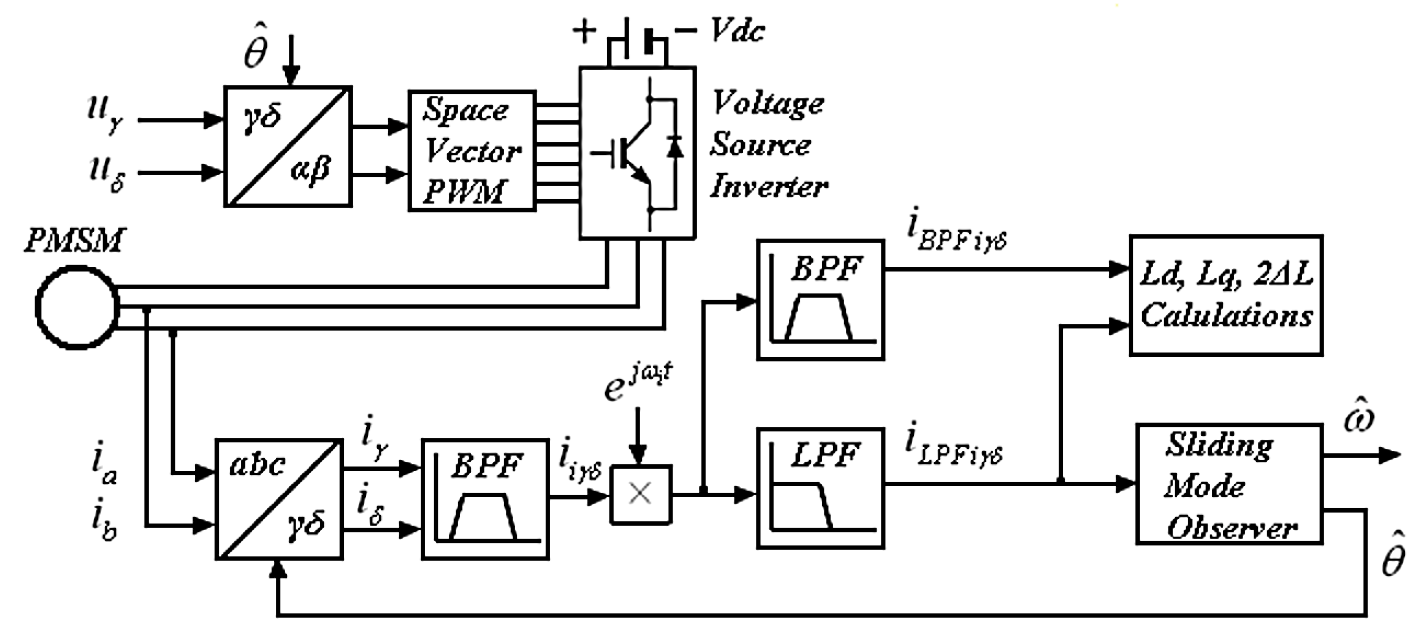
3. High-Frequency Injection (HFI) of Stator Voltage for Rotor Position Estimation

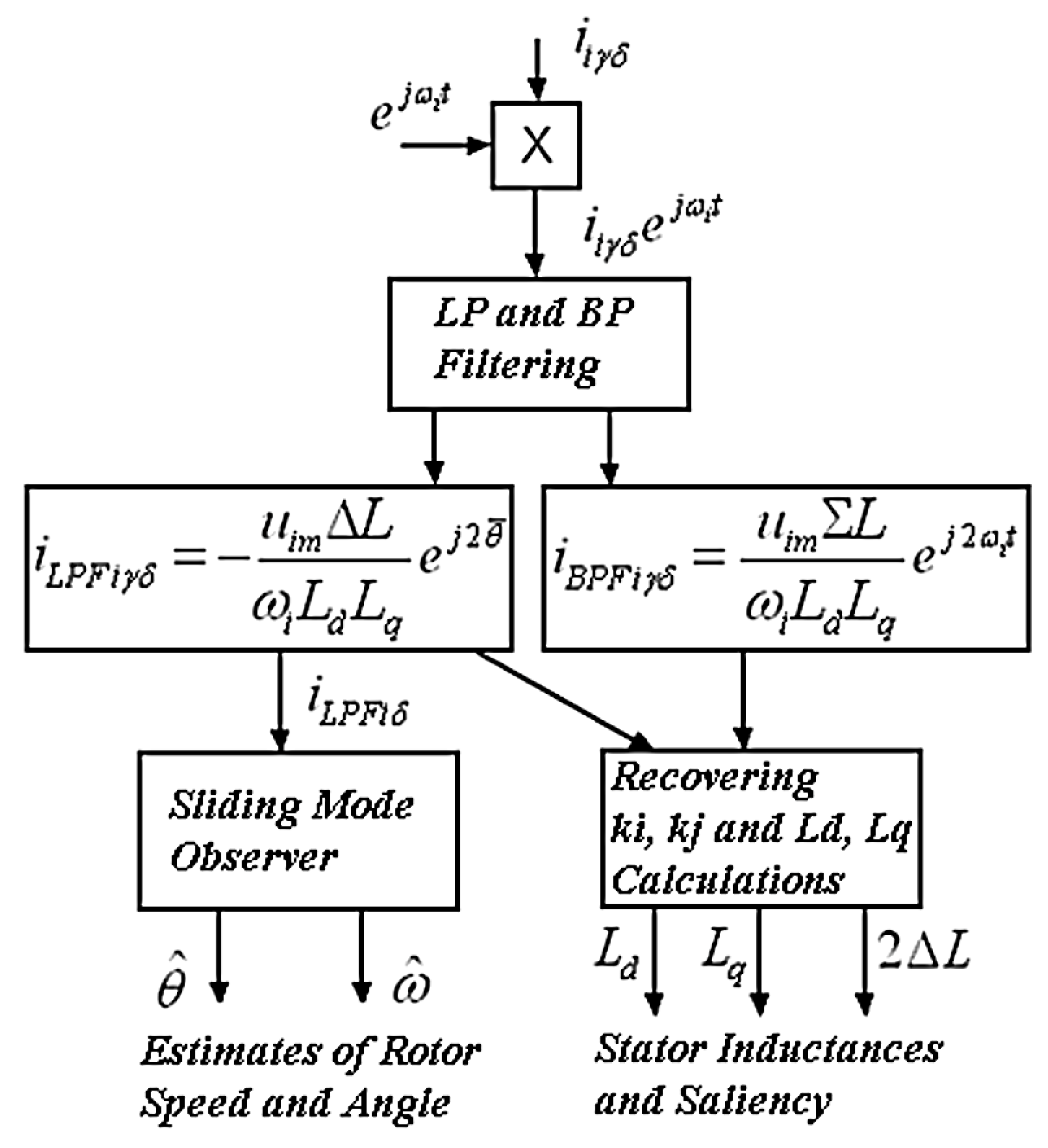
3.1. Analysis of High Frequency Stator Current in γδ Reference Frame

The variation of stator inductance due to rotor angle change implies the presence of magnetic saliency. For the injection methods, the magnetic saliency property is very important, enabling the estimation of the PMSM rotor speed and position. Measuring and processing the PMSM response of the additional HF current signal permits accurate rotor angle estimation and calculation of magnetic saliency. There are three main voltage-injection methods, namely the injection of a sinusoidal voltage signal expressed in the αβ stationary frame, the injection of a sinusoidal voltage signal in the dq frame, and the injection of discrete voltage signal in the form of pulses in the dq frame. The important characteristic of the mentioned methods is their advantage to estimate the rotor flux position at extremely low and even zero speeds. In this work, the injected voltage uiγδ is a continuous sinusoidal signal superposed on the fundamental supply frequency and expressed in γδ-estimated frame. The injected voltage vector uiγδ rotates with amplitude uim and angular speed ωi = 2πfi in relation to γδ. Therefore the HF voltage uiγδ is expressed by:
u i γ δ = u i m [ sin θ i cos θ i ] = u i m [ sin ω i t cos ω i t ] ,
where
θ i = 0 t ω i d t ,
Taking in account Equations (15) and (16), the resulting stator flux and current component due to to injected HF voltage could be calculated accordingly as follows:
λ i γ δ = 0 t ( u i γ δ r s i i γ δ ω ^ J s λ i γ δ ) d t ,
and
L γ δ i i γ δ = λ i γ δ i i γ δ = ( L γ δ ) 1 λ i γ δ ,
Substituting Equation (22) into (23), it is:
i i γ δ = ( L γ δ ) 1 [ 0 t ( u i γ δ r s i i γ δ ω ^ J s λ i γ δ ) d t ] ,
Supposing that the frequency fi is large enough, such that ω ^ < < ω i , rs << ωiLd and rs << ωiLq, terms as the HF voltage drop on the stator resistance could be eliminated. Also, since the integral of injected voltage uiγδ is the dominant term into Equation (24), the HF current calculation is simplified as:
i i γ δ ( L γ δ ) 1 [ 0 t u i γ δ d t ] = 1 L d L q [ Σ L Δ L cos 2 θ ¯ Δ L sin 2 θ ¯ Δ L sin 2 θ ¯ Σ L + Δ L cos 2 θ ¯ ] u i m ω i [ cos ω i t sin ω i t ] = u i m ω i L d L q [ Σ L cos ω i t Δ L cos 2 θ ¯ cos ω i t Δ L sin 2 θ ¯ sin ω i t Δ L sin 2 θ ¯ cos ω i t + Σ L sin ω i t + Δ L cos 2 θ ¯ sin ω i t ] = u i m ω i L d L q [ Σ L cos ω i t Δ L cos ( 2 θ ¯ ω i t ) Σ L sin ω i t Δ L sin ( 2 θ ¯ ω i t ) ] ,
Applying Euler’s formula, it will be:
i i γ δ = u i m ω i L d L q { Σ L ( cos ω i t + j sin ω i t ) Δ L [ cos ( 2 θ ¯ ω i t ) + j sin ( 2 θ ¯ ω i t ) ] } = u i m ω i L d L q [ Σ L e j ω i t Δ L e j ( 2 θ ¯ ω i t ) ] = i i γ δ p + i i γ δ n ,
where iiγδp and iiγδn are the high-frequency current components defined as:
i i γ δ p = u i m ω i L d L q Σ L e j ω i t ,
and
i i γ δ n = u i m ω i L d L q Δ L e j ( 2 θ ¯ ω i t ) ,
Here, iiγδp and iiγδn represent the HF stator current components with positive and negative frequencies, respectively. As expected, the superimposed stator current vector consists of two separate vector components, where iiγδp is the positively rotating vector with angular speed ωi and iiγδn is the negatively rotating vector with angular speed [–ωi + d(2Δθ)/dt]. It is worth noting that the average inductance is included into Equation (27), while the differential inductance ΔL and the double error of rotor position 2Δθ are included in Equation (28). Applying signal processing and filtering, the information regarding rotor position, stator inductance and magnetic saliency could be retrieved.

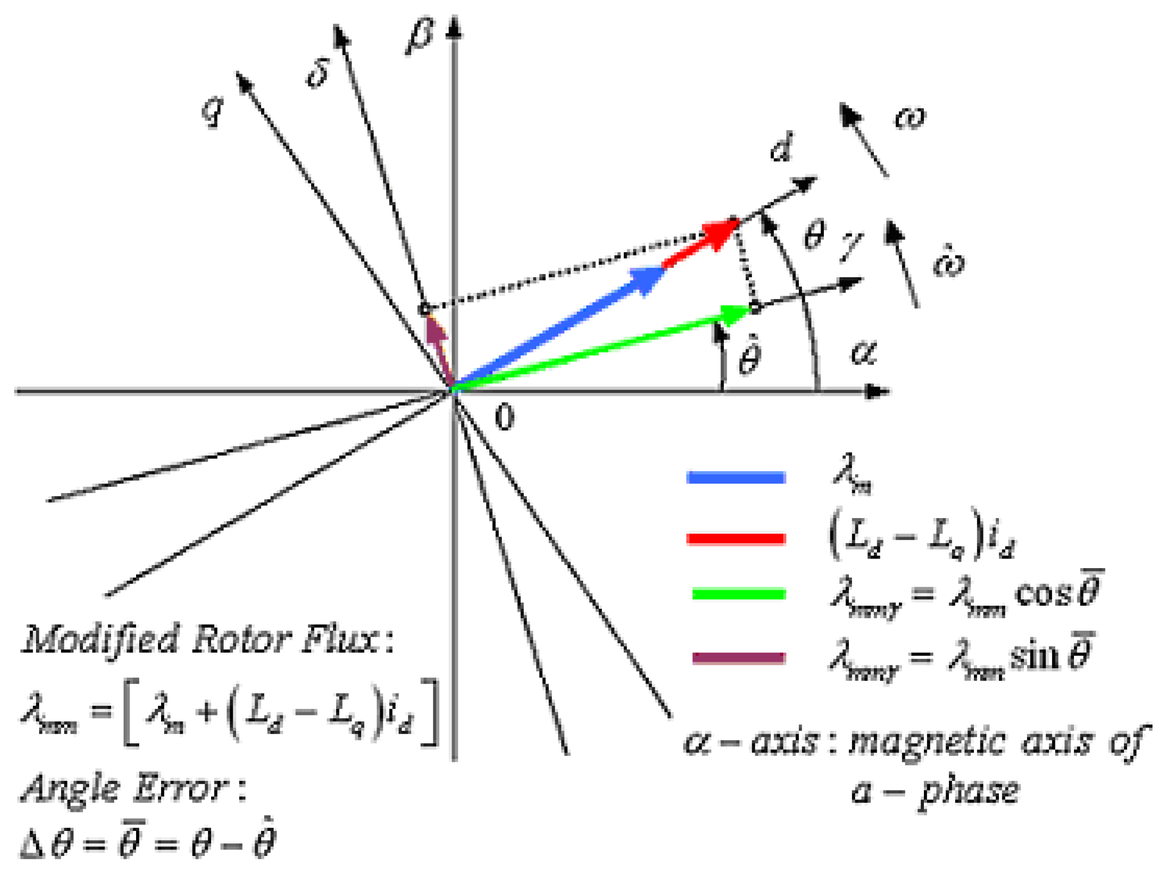
3.2. Angle Error between dq and γδ Reference Frames

Based on Equation (26) the overall estimation procedure of the rotor angle error is divided into two steps (see Figure 3). The sensorless algorithm is firstly focused on isolating the angle error information included into Equation (26), whereas in the second step it aimed to estimate rotor position through sliding mode observer (SMO). For separation of the involved error angle Δθ, both parts of Equation (26) are multiplyied by e j ω i t , i.e.,
i i γ δ e j ω i t = u i m ω i L d L q [ Σ L e j ω i t Δ L e j ( 2 θ ¯ ω i t ) ] e j ω i t = u i m ω i L d L q [ Σ L e j 2 ω i t Δ L e j 2 θ ¯ ] ,
The result in Equation (29) shows that the modulation through the multiplication by the unity vector e j ω i t leads to a vector consisting of two signals which rotate at i and 2 d θ ¯ / d t . Now, passing the resulting HF current signal in Equation (29) through a low-pass filter (LPF), the obtained current signal consists only of components proportional to sin 2 θ ¯ and cos 2 θ ¯ in a form as follows:
[ i i γ δ e j ω i t ] L P F = i L P F i γ δ = u i m Δ L ω i L d L q e j 2 θ ¯ = k i [ cos 2 θ ¯ sin 2 θ ¯ ] [ k i cos 2 θ ^ k i sin 2 θ ^ ] k i 2 θ ¯ ,
where
k i = u i m Δ L ω i L d L q ,
This implies that angle information could be recovered from the angle difference obtained through filtering off directly the modulated HF stator current in Equation (29). Obviously, the low-pass filtered signal in Equation (30) is in a convenient form to be utilized for speed and position estimation. In the next step, the LPF output signals are used as inputs of a SMO to derive the speed and position of the PMSM rotor flux (see Figure 3). In a similar manner, the first part containing the HF current signal in Equation (29) is also isolated after passing the signal i i γ δ e j ω i t through a band-pass filter (BPF). Thus, BPF output consists only of the HF current component given by:
[ i i γ δ e j ω i t ] B P F = i B P F i γ δ = u i m Σ L ω i L d L q e j 2 ω i t = k j [ cos 2 ω i t sin 2 ω i t ] ,
where
k j = u i m Σ L ω i L d L q ,
Considering Equations (31) and (33), it follows that ki depends on the inductances Ld, Lq and differential inductance, whereas kj represents the amplitude of the BPF output depending on the inductances Ld, Lq and their average. The block diagram of current signal processing is shown in Figure 3. As illustrated, only the δ component of LPF output is needed for speed/position estimation, while the parameters ki and kj from both LPF and BPF are used to compute the inductances Ld, Lq and saliency (LdLq).

3.3. Angle Error of PMSM Rotor Flux in γδ Reference Frame

Although, there are available two orthogonal signals from Equation (29), k i cos 2 θ ¯ and k i sin 2 θ ¯ , the speed and position estimation algorithm requires only the k i sin 2 θ ¯ component. Figure 4 shows the observer structure for speed and position tracking in details. Considering the iLPFiδ component from Equation (30), the estimated angle of rotor flux is related to the real one through the following relation (3rd Ptolemy’s identity/the difference formula for sine, see Figure 4):
i L P F i δ = k i sin 2 θ ¯ = k i sin ( 2 θ 2 θ ^ ) = k i sin 2 θ cos 2 θ ^ k i cos 2 θ sin 2 θ ^ ,
Equation (34) is interpreted schematically in Figure 4 implying how the angle error is equivalently connected to real and estimated speed by means of iLPFiδ. If the difference between the estimated and actual rotor flux positions is small, the current iLPFiδ can be approximated by k i 2 θ ¯ because sin 2 θ ¯ 2 θ ¯ = 2 Δ θ = 2 θ 2 θ ^ . This implies that iLPFiδ is almost directly proportional to Δθ for the small angle difference.

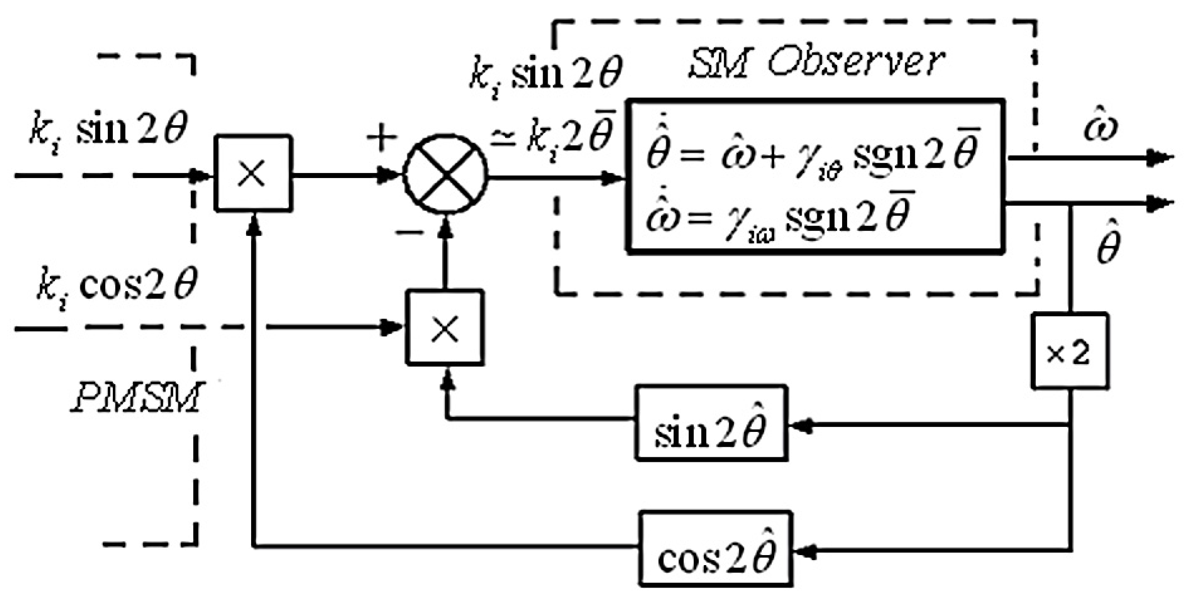
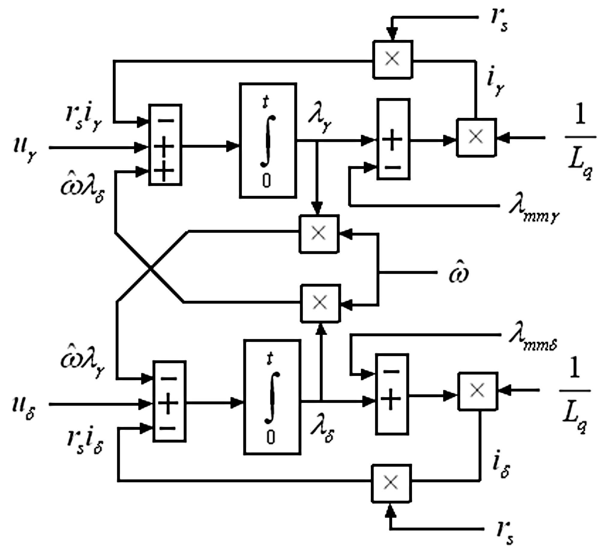
3.4. Design of Sliding Mode Observer (SMO) for Estimation of Rotor Flux Angle and Speed

Among the proposed observer schemes, the sliding mode observers (SMO) are widely studied in the literature and applied on a plethora of industrial applications. The main advantage of sliding mode methodology is that provides robustness and fast convergence in finite time under system disturbances and modeling uncertainties. In designing the SMO, its structure typically includes two steps, namely the sliding manifold and control law. Here, the sliding manifold design is determined choosing the rotor angle and speed errors, θ ¯ and ω ¯ , as sliding surfaces. Also the control law consists of the sign function sgn 2 θ ¯ , while the observer gains are defined as γiθ and γiω for angle and speed tracking, respectively. In addition, the principles of equivalent control approach are also used in sliding mode observer stability after reaching phase. Based on Equation (34), the proposed angle/speed observer is determined as follows:
θ ^ ˙ = ω ^ + γ i θ sgn 2 θ ¯ ,
and
ω ^ ˙ = γ i ω sgn 2 θ ¯ ,
where sgn 2 θ ¯ is the signum function 2 θ ¯ . In Figure 4, the input and output signals of SMO are schematically illustrated using an equivalent block diagram.

3.4.1. SMO Dynamics and Stability

Using the above sliding manifold and Equations (35) and (36), the SMO dynamics could be expressed as:
θ ¯ ˙ = θ ˙ θ ^ ˙ = ω ω ^ γ i θ sgn 2 θ ¯ = ω ¯ γ i θ sgn 2 θ ¯ ,
and
ω ¯ ˙ = ω ˙ ω ^ ˙ = γ i ω sgn 2 θ ¯ ,
Let us suppose that γiθ is large enough, such that:
γ i θ > > | ω ¯ | ω ¯ ,
i.e., γiθ is an upper bound of ω ¯ , then:
( 37 ) θ ¯ ˙ = 0 ω ¯ = γ i θ ( sgn 2 θ ¯ ) e q ( sgn 2 θ ¯ ) e q = ω ¯ γ i θ ,
Here, the term (.)eq represents the equivalent control. Eventually the equivalent control could be used as input for the speed estimation procedure. Substituting Equation (36) into (38) it results that:
ω ¯ ˙ = γ i ω ( sgn 2 θ ¯ ) e q = γ i ω γ i θ ω ¯ ,
This stability analysis implies that the SMO defined in Equations (35) and (36) is asymptotically stable with errors tending to zero. Considering Equation (41), it is obvious that the developed approach of sliding mode observer is implemented as a reduced order asymptotic observer by means of the equivalent control.
Considering the reaching phase, the sliding surface θ ¯ = 0 is reached at limited time tr given by:
t r 2 V 1 / 2 ( 0 ) ξ = 2 | θ ¯ ( 0 ) | ( γ i θ P d ) ,
where
ξ = 2 ( γ i θ P d ) ,
The Pd represents the upper limit of the bounded disturbance regarding ω ¯ . Also taking in account Equation (41), a general solution converges to zero asymptotically, described by:
ω ¯ ˙ = γ i ω γ i θ ω ¯ ω ¯ ( t ) = ω ¯ ( 0 ) e ( γ i ω / γ i θ ) t ,
Inspecting Equation (42), it obvious that the maximum time tr is directly proportional to the initial angle error | θ ¯ ( 0 ) | , while it is directly inverserly proportional to the gain γiθ. In addition, the speed error converges asymptotically faster to zero as the rate (γ/ωiθ) increases [30].

3.4.2. Approximation of sgn(.) Function-Chattering Reduction

Although a sliding mode observer offers advadages and enhanced stability properties, the applied control signal causes high-frequency oscillations after the system states, θ ¯ and ω ¯ , reach the sliding surfaces. Such undesirable oscillations are called a chattering phenomenon and they affect negatively sliding mode applications. As a consequence, the chattering excites the system-unmodeled dynamics leading probably to large estimation errors or observer malfunction. Conventionally, the control law is substituted by a smooth continuous function to approximate the discontinuous sign function. This could succeed in dealing with the serious disadvantage of chattering phenomenon. Among the suggested solutions, the hyperbolic tangent tanh(.) is a relatively simple smooth approximation of the sign function in reducing chattering, since sgn 2 θ ¯ tanh ( k 2 θ ¯ ) for k >> 1.

4. Estimation of PMSM Inductances and Magnetic Saliency

4.1. Calculating the Parameters ki and kj

Since the γδ rotating reference frame is orthogonal, the magnitude of the parameter ki is calculated as the hypotenuse of a right triangle whose legs are the components of the LPF output (Pythagorean Theorem), that is the square root of the squares of iLPFγ and iLPFδ currents in Equation (30), i.e.,
k i = [ ( i L P F γ ) 2 + ( i L P F δ ) 2 ] sgn ( Δ L ) ,
Alternatively, the ki can also estimated from iLPFiγ in Equation (30), as the angle error tends to zero (i.e., k i cos 2 θ ¯ = k i ). The sign of ki is opposite of this of ΔL, i.e., for ΔL > 0, it is ki < 0 or for ΔL < 0, it is ki > 0. Normally, if the PMSM is operating as a motor, it will be ΔL < 0 and thus ki > 0. In the same manner, the parameter kj is positive and it is obtained from the components of the BPF output in γδ frame, i.e.,
k j = [ ( i B P F γ ) 2 + ( i B P F δ ) 2 ] ,
Regarding Equations (45) and (46), it results that magnitudes of both parameters ki and kj essentially represent the amplitudes of the low and high frequency current signals in Equation (29). Also comparing the magnitudes and absolute values of ki and kj, it is kj > ki and |kj| > |ki|, since ΣL > −ΔL and ΣL >L|.

4.2. Expressing dq Impedances as Functions of the ki and kj Parameters

Inspecting Equations (31) and (33), it can be noted that ki and kj are directly analogous to ΔL and ΣL respectively with ratio coefficient ±um/(ωiLdLq). Additionally, the sum and difference of ΣL and ΔL are equal to Ld and Lq i.e., (ΣL + ΔL) = [(Ld + Lq)/2] + [(Ld − Lq)/2] = Ld and (ΣL − ΔL) = [(Ld + Lq)/2] − [(Ld − Lq)/2] = Lq. This implies that the d-axis and q-axis inductances of PMSM can be easily calculated in terms of the ki and kj parameters. Adding by parts Equations (31) and (33), it follows that:
k j + k i = u i m ( Σ L Δ L ) ω i L d L q = u i m L q ω i L d L q = u i m ω i L d ,
Now solving Equation (47) for Ld, the d-axis inductance is given as
( 47 ) L d = u i m ω i ( k j + k i ) ,
Also, subtracting by parts Equation (31) from Equation (33), the following results:
k j k i = u i m ( Σ L + Δ L ) ω i L d L q = u i m L d ω i L d L q = u i m ω i L q ,
Subsequently, solving Equation (49) for Lq, this is:
( 49 ) L q = u i m ω i ( k j k i ) ,

4.3. Expressing the PMSM Magnetic Saliency (Ld − Lq) as Function of Parameters ki and kj

Substituting Ld and Lq from Equations (48) and (50), the magnetic saliency can be written as follows:
( L d L q ) = 2 Δ L = u i m ω i [ 1 ( k j + k i ) + 1 ( k j k i ) ] = u i m ω i [ 2 k j ( k j 2 k i 2 ) ] ,
Equation (51) allows the calculation of PMSM magnetic saliency using the parameters ki and kj. After accomplishing the calculations from Equation (45) to Equation (51), it is feasible to estimate both inductances Ld, Lq and magnetic saliency. The analysis above implies that the stator inductance changes or even magnetic fault diagnosis could be monitored by means of the proposed HFI method.

5. Simulation Results and Discussion

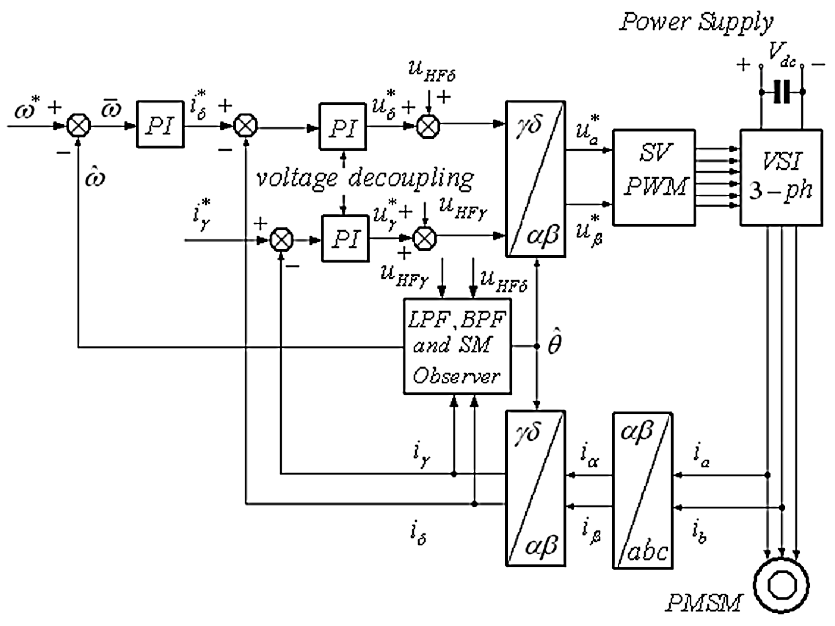
5.1. Description of Simulated PMSM Model and Control System

For test and evaluation purposes, a vector control is employed, whose block diagram is depicted in Figure 1. Modeling and design of the proposed sensorless control scheme is implemented using Simulink/Matlab application. Mainly, the total model structure including dynamics is described in Figure 1. The simulated PMSM model is based on the primitive Equations (5)–(19) associated with the γδ reference frame, while observer model uses Equations (30) and (34)–(36) to estimate both rotor speed and position. In addition, stator inductances and magnetic saliency are calculated using Equations (45)–(51) after suitable processing, i.e., modulating and filtering the stator currents (see Figure 3 and Figure 5). The simulated model was tested and verified using the PMSM parameters listed in Table 1. Considering Equation (31) and Ld > Lq, i.e., ΔL > 0, the sign of ki is negative in this particular machine. A three-leg VSI drives the PMSM fed with 400 V dc. In simulation tests, the output voltage of the VSI is modulated by means of SVPWM algorithm, while the switching frequency is set at 5 kHz. As it is demonstrated in Figure 1, the HF voltage signals are added with the uγ* and uδ* voltage references. In aiming to precisely estimate the rotor position, the frequency and amplitude of the injected signal is set at 1 kHz and 50 V, respectively. Considering the control law of the SMO, the parameter k of the hyperbolic tangent function tanh ( k 2 θ ¯ ) is set equal to 10, while the observer performance has been attained for gains γiθ = 40 and γiω = 5. A diagram of the developed PMSM model in γδ is demonstrated in Figure 6.
In future work, hardware implementation of the studied approach should be based on a development board equipped with powerful digital signal processor (DSP) or multi processor unit (MPU). For example, a single-board solution is the DS1104 research and development (R&D) Controller Board of dSPACE. The Real-Time Interface (RTI) software provided allows direct implementation of the developed Simulink models on the real-time hardware. Data collection, communication and control are succeeded in through the available interfaces (A/D or D/A converter channels) including the PWM outputs.

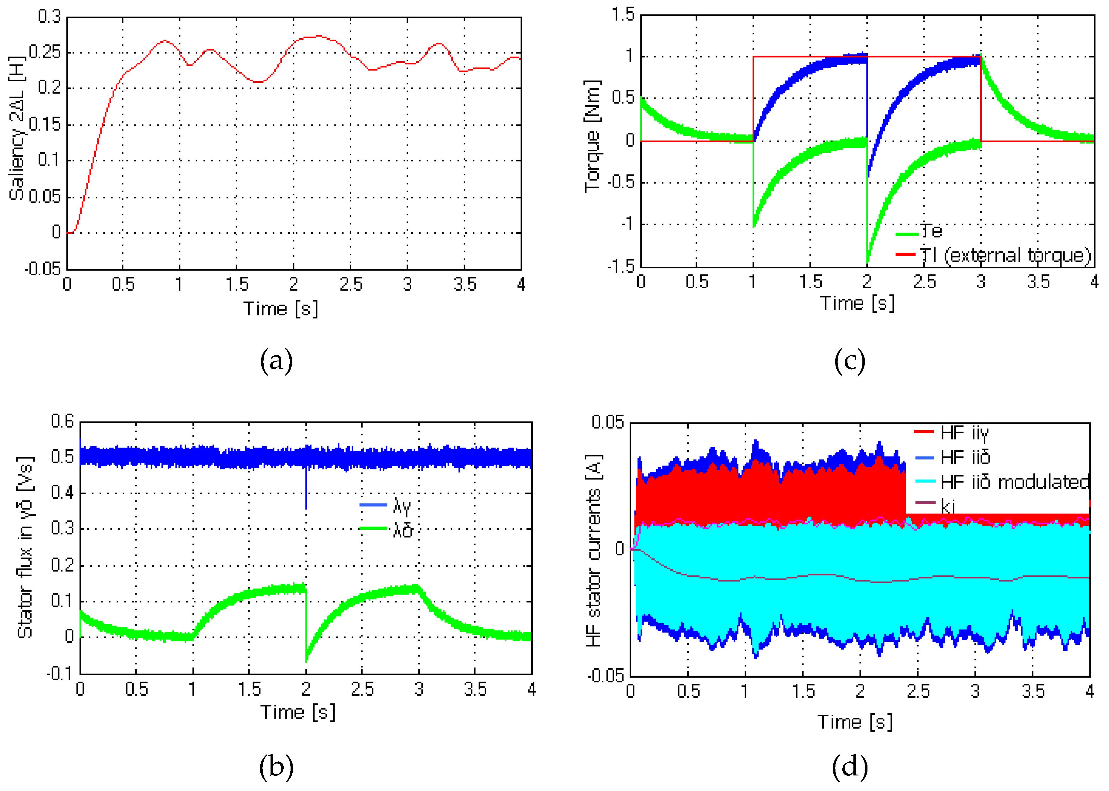
5.2. Response at Very Low Speed and Standstill

Simulation results are presented in Figure 7 without external torque disturbance. The reference speed is changed stepwise from 0 rad/s to π/2 rad/s (0.5 Hz) and at t2 = 2s it changed from π/2 rad/s to 0 rad/s (standstill). Figure 7a,b shows the estimated rotor speed and stator currents, respectively, while HF stator currents iiγδ, the modulated and iLPFiγ are displayed in Figure 7c. In Figure 7a, it is demonstrated that the SMO converges very fast with accurate speed estimation. Also, the response of stator current iγδ is shown in Figure 7b including its HF components. The ki in Figure 7c is obtained from the iLPFiγ from Equation (30), i.e., after LP filtering the γ-component of modulated HF current. At standstill operation without external torque disturbance in particular, the observer error remains very small preserving its excellent performance. The inspection of the iγδ current waveforms shows that the observer-controller system behaves well with a very small chattering introduced in iγ due to the fast switching of the control input in the SMO. However the usage of hyperbolic tangent function, tanh(.), has greatly improved the currents’ response while keeping the advantageous characteristics of the SMO.

5.3. Very Low Speed Response with Torque Load

Simulation results presented in Figure 7d-f show the PMSM speed response during speed changes in the presence of external torque 1 Nm. Here the speed is changed stepwise from 0 rad/s to π/2 rad/s (0.25 Hz) and from π/2 rad/s to -π rad/s (0.5 Hz) at t2 = 2s. Also the external torque of 1 Nm is applied at t1 = 1 s and it is removed at t3 = 3 s. The rotor speed and angle are shown in Figure 7d,e, respectively, while the HF stator currents including modulated and ki are shown in Figure 7f. The very small speed and angle errors show the robustness of the proposed estimation scheme. Also, as expected the frequency of derived current signals is double that of the injected one after modulation. It is worth noting here that during the transition from π/2 rad/s to -π rad/s the observer behavior is robust and stable even in presence of torque disturbance. The observer keeps converging fast with very small angle errors between the synchronous dq (real) and γδ estimated reference frames.

5.4. Flux and Torque Response with Saliency Estimation at Very Low Speed

The stator flux and torque responses are presented in Figure 8b,c respectively. Here, the speed changes stepwise from 0 rad/s to π rad/s and from π rad/s to −π rad/s at t2 = 2 s in presence of 1 Nm as external torque disturbance applied at t1 = 1 s and then removed at t3 = 3 s. An estimation of the saliency 2ΔL is demonstrated in Figure 8a, while HF stator currents with estimation of ki parameter are shown in Figure 8d. It can be observed that the estimated saliency is very close to the real one, implying the accuracy of the proposed estimation scheme. However this accuracy is mostly affected on the information extracted for both ki and kj parameters.

6. Conclusions

A novel sensorless algorithm was developed and tested for the speed and position of a PMSM based on HFI methodology. Using the γδ modified PMSM model, the proposed scheme was evaluated as an effective sensorless approach embedding appropriately the magnetic saliency terms of the modified rotor flux into a new inductance matrix in γδ. Applying directly a HF voltage signal to a VSI, the resulting stator current was utilized to extract rotor angle information through LPF and sliding mode observer. Based on the advantages of the SMO structure, the speed/position observer converges very fast in finite time even for zero speed command at presence of torque disturbance (low and very low speed range, 0.5–0Hz). In addition, the LP and BP filtered signals were used in a simple manner to track stator inductances and magnetic saliency. Simulation results demonstrate the estimation scheme efficiency verifying the observer robustness at very low and even at standstill operation. The proposed algorithm performed well with exceptional convergence characteristics providing accurate estimates of dq inductances and saliency.

Author Contributions

The author conceived of the presented idea, developed the theory and performed the computations. Also, he verified the proposed method through simulations and discussed the results/findings of this work that have been included into the final manuscript. The author have read and agreed to the published version of the manuscript

Funding

This research received no external funding.

Conflicts of Interest

The authors declare no conflict of interest.

References

  1. Morimoto, S.; Kawamoto, K.; Sanada, M.; Takeda, Y. Sensorless control strategy for salient-Pole PMSM based on extended EMF in rotating reference frame. IEEE Trans. Ind. Appl. 2002, 38, 1054–1061. [Google Scholar] [CrossRef]
  2. Yang, S.; Lorenz, R. Surface permanent-magnet machine self-Sensing at zero and low speeds using improved observer for position, velocity, and disturbance torque estimation. IEEE Trans. Ind. Appl. 2012, 48, 151–160. [Google Scholar] [CrossRef]
  3. Wang, X.; Kennel, R.M. Analysis of permanent-Magnet machine for sensorless control based on high-frequency signal injection. In Proceedings of the IEEE 7th International Power Electronics and Motion Control Conference (IPEMC 2012), Harbin, China, 2–5 June 2012; pp. 2367–2371. [Google Scholar]
  4. Preindl, M.; Schaltz, E. Sensorless Model Predictive Direct Current Control Using Novel Second-Order PLL Observer for PMSM Drive Systems. Ind. Electron. IEEE Trans. 2011, 58, 4087–4095. [Google Scholar] [CrossRef]
  5. Piippo, A.; Salomäki, J.; Luomi, J. Signal injection in sensorless PMSM drives equipped with inverter output filter. In Proceedings of the Fourth Power Conversion Conference (PCC 2007), Nagoya, Japan, 2–5 April 2007; pp. 1105–1110. [Google Scholar]
  6. Hammel, W.; Kennel, R.M. Position sensorless control of PMSM by synchronous injection and demodulation of alternating carrier voltage. In Proceedings of the 2010 First Symposium on Sensorless Control for Electrical Drives (SLED 2010), Padova, Italy, 9–10 July 2010; pp. 56–63. [Google Scholar]
  7. Trancho, E.; Ibarra, E.; Arias, A.; Salazar, C.; Lopez, I.; de Guereñu, A.D.; Peña, A. A novel PMSM hybrid sensorless control strategy for EV applications based on PLL and HFI. In Proceedings of the 42nd Annual Conf. of the IEEE Industrial Electronics Society (IECON 2016), Florence, Italy, 23–26 October 2016. [Google Scholar]
  8. Tuovinen, T.; Hinkkanen, M.; Harnefors, L.; Luomi, J. Comparison of a reduced-Order observer and a full-Order observer for sensorless synchronous motor drives. IEEE Trans. Ind. Appl. 2012, 48, 1959–1967. [Google Scholar] [CrossRef] [Green Version]
  9. Park, Y.; Sul, S. Sensorless control method for PMSM based on frequency-adaptive disturbance observer. IEEE J. Emerg. Sel. Top. Power Electron. 2014, 2, 143–151. [Google Scholar] [CrossRef]
  10. Wang, G.; Zhan, H.; Zhang, G.; Gui, X.; Xu, D. Adaptive compensation method of position estimation harmonic error for EMF-based observer in sensorless IPMSM drives. IEEE Trans. Power Electron. 2014, 29, 3055–3064. [Google Scholar] [CrossRef]
  11. Betin, F.; Capolino, G.A.; Casadei, D.; Kawkabani, B.; Bojoi, R.I.; Harnefors, L.; Levi, E.; Parsa, L.; Fahimi, B. Trends in electrical machines control samples for classical, sensorless, and fault-Tolerant techniques. IEEE Ind. Electron. Mag. 2014, 8, 43–55. [Google Scholar] [CrossRef]
  12. Huang, K.; Zhou, L.; Zhou, T.; Huang, S. An enhanced reliability method for initial angle detection on surface mounted permanent magnet synchronous motors. Trans. China Electrotech. Soc. 2015, 1, 45–51. [Google Scholar]
  13. Bolognani, S.; Calligaro, S.; Petrella, R. Design issues and estimation errors analysis of back-EMF-Based position and speed observer for SPM synchronous motors. IEEE J. Emerg. Sel. Top. Power Electron. 2014, 2, 159–170. [Google Scholar] [CrossRef]
  14. Pacas, M. Sensorless drives in industrial applications. IEEE Ind. Electron. Mag. 2011, 5, 16–23. [Google Scholar] [CrossRef]
  15. Foo, G.; Rahman, M.F. Sensorless sliding mode MTPA control of an IPM synchronous motor drive using a sliding-mode observer and HF signal injection. IEEE Trans. Ind. Electron. 2010, 57, 1270–1278. [Google Scholar] [CrossRef]
  16. Staines, C.S.; Caruana, C.; Raute, R. A review of saliency-based sensorless control methods for alternating current machines. IEEJ J. Ind. Appl. 2014, 3, 86–96. [Google Scholar] [CrossRef] [Green Version]
  17. Chen, G.; Yang, S.; Hsu, Y.; Li, K. Position and Speed Estimation of Permanent Magnet Machine Sensorless Drive at High Speed Using an Improved Phase-Locked Loop. Energies 2017, 10, 1571. [Google Scholar] [CrossRef] [Green Version]
  18. Chen, Z.; Tomita, M.; Ichikawa, S.; Doki, S.; Okuma, S. Sensorless control of interior permanent magnet synchronous motor by estimation of an extended electromotive force. Conf. Rec. IEEE-IAS Annu. Meet. 2000, 3, 1814–1819. [Google Scholar]
  19. Chen, ZC.; Tomita, M.; Doki, S.; Okuma, S. An extended electromotive force model for sensorless control of interior permanent-Magnet synchronous motors. IEEE Trans. Ind. Electron. 2003, 50, 288–295. [Google Scholar] [CrossRef]
  20. Kim, H.; Harke, M.C.; Lorenz, R.D. Sensorless control of interior permanent-magnet machine drives with zero-Phase lag position estimation. IEEE Trans. Ind. Appl. 2003, 39, 1726–1733. [Google Scholar]
  21. Ilioudis Vasilios, C. Sensorless Control Applying Signal Injection Methodology on Modified Model of Permanent Magnet Synchronous Machine. In Proceedings of the Conference on Control, Decision and Information Technologies (CoDIT 2019), Paris, France, 23–26 April 2019; pp. 1935–1940. [Google Scholar]
  22. Cho, Y. Improved Sensorless Control of Interior Permanent Magnet Sensorless Motors Using an Active Damping Control Strategy. Energies 2016, 9, 135. [Google Scholar] [CrossRef] [Green Version]
  23. Piippo, A.; Luomi, J. Inductance harmonics in permanent magnet synchronous motors and reduction of their effects in sensorless control. In Proceedings of the XVII International Conference on Electric Machines (ICEM 2006), Chania, Crete Island, Greece, 2–5 September 2006. [Google Scholar]
  24. Corley, M.; Lorenz, R.D. Rotor Position and Velocity Estimation for a Salient-Pole Permanent Magnet Synchronous Machine at Standstill and High Speeds. IEEE Trans. Ind. Appl. 1998, 34, 784–789. [Google Scholar] [CrossRef]
  25. Zhu, Z.Q.; Gong, L.M. Investigation of effectiveness of sensorless operation in carrier signal injection based sensorless control Methods. IEEE Trans. Ind. Electron. 2011, 8, 3431–3439. [Google Scholar] [CrossRef]
  26. Murakami, S.; Shita, T.; Ohto, M.; Ide, K. Encoderless servo drive with adequately designed IPMSM for pulse-voltage-injection-Based position detection. IEEE Trans. Ind. Electron. 2012, 48, 1922–1930. [Google Scholar] [CrossRef]
  27. Schoonhoven, G.; Uddin, M.N. Harmonic Injection-Based adaptive control of IPMSM motor drive for reduced motor current THD. IEEE Trans. Ind. Appl. 2017, 53, 483–491. [Google Scholar] [CrossRef]
  28. Chen, Jy.; Yang, Sh.; Tu, Ka. Comparative Evaluation of a Permanent Magnet Machine Saliency-Based Drive with Sine-Wave and Square-Wave Voltage Injection. Energies 2018, 11, 2189. [Google Scholar] [CrossRef] [Green Version]
  29. Hejny, R.W.; Lorenz, R.D. Evaluating the practical low-Speed limits for back-EMF tracking-Based sensorless speed control using drive stiffness as a key metric. IEEE Trans. Ind. Appl. 2011, 47, 1337–1343. [Google Scholar] [CrossRef]
  30. Shtessel, Y.B. Sliding Mode Control with Applications: Tutorial. In Proceedings of the ICEECSAS-2008, UNAM, Mexico City, Mexico, 12 November 2008. [Google Scholar]
  31. Zidat, F.; Lecointe, J.P.; Morganti, F.; Brudny, J.F.; Jacq, T.; Streiff, F. Non Invasive Sensors for Monitoring the Efficiency of AC Electrical Rotating Machines. Sensors 2010, 10, 7874–7895. [Google Scholar] [CrossRef] [PubMed] [Green Version]
  32. Henao, H.; Capolino, G.A.; Razik, H. Analytical Approach of the Stator Current Frequency Harmonics Computation for Detection of Induction Machine Rotor Faults. In Proceedings of the Symposium on Diagnostic for Electrical Machines, Power Electronics and Drives, SDEMPED, Atlanta, GA, USA, 24–26 August 2003; pp. 259–264. [Google Scholar]
  33. Briz, F.; Degner, M.W.; Zamarrón, A.; Guerrero, J.M. Online Diagnostics in Inverter-Fed AC Machines Using High-Frequency Signal Injection. IEEE Trans. Ind. Appl. 2004, 40, 1109–1117. [Google Scholar] [CrossRef]
  34. Wu, X.; Wang, H.; Huang, S.; Huang, K.; Wang, L. Sensorless Speed Control with Initial Rotor Position Estimation for Surface Mounted Permanent Magnet Synchronous Motor Drive in Electric Vehicles. Energies 2015, 8, 11030–11046. [Google Scholar] [CrossRef] [Green Version]
  35. Lv, C.; Liu, Y.; Hu, X.; Guo, H.; Cao, D.; Wang, Fe. Simultaneous Observation of Hybrid States for Cyber-Physical Systems: A Case Study of Electric Vehicle Powertrain. IEEE Trans. Cybern. 2018, 48, 2357–2367. [Google Scholar]
Figure 1. Block diagram of permanent magnet synchronous machine (PMSM) sensorless control based on voltage high-frequency injection (HFI) with LPF, BPF (low- and band-pass filtering) and a sliding mode observer (SMO) for speed and position.
Machines 08 00014 g001
Figure 2. Vector diagram of the modified rotor flux λmm in dq and γδ (rotating) reference frames as they related to αβ (stationary) reference frame with α representing magnetic axis of phase a.
Machines 08 00014 g002
Figure 3. The description of high-frequency (HF) current processing in flow chart form: (1) stator current modulation, (2) low-pass and band-pass filtering (LPF, BPF), (3) speed/position estimation and (4) inductances and saliency calculation.
Machines 08 00014 g003
Figure 4. An equivalent block diagram for PMSM speed and position estimation based on sliding mode observer (SMO).
Machines 08 00014 g004
Figure 5. The observer and power supply blocks in more details as they used in simulation for PMSM sensorless control.
Machines 08 00014 g005
Figure 6. The PMSM model in γδ reference frame that is used as basis to form the sliding mode observer (SMO) for speed and position estimation.
Machines 08 00014 g006
Figure 7. (Left) PMSM responses for speed change from 0 rad/s to π/2 rad/s (0.25 Hz) and at t2 = 2 s from π/2 rad/s to 0 rad/s without external torque: (a) angular speed, (b) stator current and (c) HF stator currents with estimation of ki parameter. (Right) PMSM responses for speed change from 0 rad/s to π/2 rad/s (0.25 Hz) and at t2 = 2 s from π/2 rad/s to −π rad/s (−0.5 Hz), while an external torque of 1 Nm is applied at t1 = 1 s and removed at t3 = 3 s: (d) angular speed, (e) angular position and expansion of HF stator currents with estimation of ki parameter in (f).
Machines 08 00014 g007
Figure 8. PMSM responses for speed change from 0 rad/s to π rad/s (0.5 Hz) and at t2 = 2 s from π rad/s to -π rad/s (-0.5 Hz), while an external torque of 1 Nm is applied at t1 = 1 s and removed at t3 = 3 s: (a) saliency estimation, (b) stator flux, (c) torque (electrical and load) and (d) HF stator currents with estimation of ki parameter.
Machines 08 00014 g008
Table 1. Parameters of Permanent Magnet Synchronous Machine (PMSM).
SymbolQuantityExpressed in SI
SApparent power5.5 kVA
cosφElectric power coefficient0.8
Vl-lLine to line voltage380 V
rsStator resistance2.5 Ω
Lmdd-axis magnetizing inductance 0.360 H
Ldd-axis inductance0.400 H
Lqq-axis inductance 0.210 H
λmPermanent Magnet Flux 0.5 Vs (or Wb)
JMoment of inertia 0.089 kgm2
pMagnetic pole pairs1
ωmMechanical angular speed3000 rpm

